Microwave Imaging for Half-Space Conductors Using the Whale Optimization Algorithm and the Spotted Hyena Optimizer

Abstract

This research implements the whale optimization algorithm (WOA) and spotted hyena optimizer (SHO) in inverse scattering to regenerate the conductor shape concealed in the half-space. TM waves are irradiated from the other half-space to a perfect conductor with an unknown shape buried in one half-space. The scattered field measured outside the conductor surface with the boundary condition is used to reconstruct the object using the WOA and SHO algorithms. Several scenarios of reconstruction accuracy were compared for the WOA and SHO. The numerical simulations prove that the WOA has a better reconstruction capability.

1. Introduction

In recent years, electromagnetic imaging has been extensively applied in the medical imaging fields, such as CT and MR. In medical imaging, for instance, the technology is superior to that of X-ray, with a better performance in scattered field information collection. This has motivated scholars to research deeper into related studies, with significant progress having been achieved. In general, the methods for solving electromagnetic scattering problems can be categorized into two main domains: the first is the approximate solution method and the second is the rigorous numerical method. The main approximate imaging theory for conductors is described by Bojarski’s equation [1,2,3,4], which was proposed by Bojarski in 1967 based on the assumption of physical optics. This equation shows that there is a Fourier transformation between the backscattered field and the shape of the object, so that the image can be reconstructed using the scattered field. Since this method is only applicable to far-field imaging, some scholars have extended it to near-field imaging [5]. However, these methods are based on the assumptions of physical optics, and only one scattering condition is considered. The image object must be “convex” with a smooth surface and the size must be much larger than the wavelength. All these problems have limited its widespread application. This research can be applied to biomedical imaging (e.g., shapes and sizes of breast cancer and tumors), remote sensing and non-destructive testing. It is worth mentioning that biomedical imaging on breast cancer has been widely discussed in recent years.

As far as the rigorous methods in the inverse scattering theory are concerned, most of them are based on an integral equation with the moment method [6,7,8,9,10,11,12,13,14]. Depending on the properties of the object, inverse scattering theory can be divided into two cases: conductors and dielectric objects. In the case of conductors, the inverse scattering problem is usually transformed into an optimization problem. The first form of the objective function is defined by the root-mean-square error between the measured and calculated scattered fields [7,8,9,10]. By searching for the minimum value of the objective function, an optimal solution satisfying the boundary conditions can be found. The second form of the objective function is composed of two summations: one is the objective function of the first type and the other is the root-mean-square error of the set of integral equations satisfying the boundary condition [11,12,13,14]. In addition, a regularization term can be added after the above objective functions to remove the ill-posedness. Then, the two forms of objective functions are completed by numerical iterations, such as the Newton–Kantorovitch method [7,8,9], the Levenberg–Marquardt algorithm [11,12,13], the successive overrelaxation method [14] and discrete dipole approximation [15]. However, almost all of these rigorous methods search for the solution by the gradient of the objective function. Therefore, when the preliminary estimation is further away from the real value, the solution is often a local extreme rather than a global extreme.

A vast amount of literature on the heuristic algorithm has been published recently [16,17,18,19,20,21,22,23,24,25,26,27,28,29]. The first was published in 1975, when Holland proposed the concept and theoretical basis of genetic evolution based on Darwin’s concept of “natural selection”, using the genetic mechanism of “survival of the fittest” to simulate the biological evolutionary process of genetic selection and natural elimination to find the best solution by a random search [16]. In 2018, Chiu et al. applied the self-adaptive dynamic differential evolution (SADDE) method to reconstruct two-dimensional dielectric objects and highlighted its robustness and searching speed [17]. The whale algorithm, which simulates the hunting behavior of humpback whales for optimal search, is a new bionic algorithm proposed by Mirjalili and Lewis in 2016 [19]. Before the publication of their paper, there was no research on the whale algorithm. The search formulation of the proposed whale algorithm was able to explore random solutions in space. Subsequently, Ling et al. proposed a levy flight-based whale algorithm. Although this algorithm could efficiently solve low-dimensional single-peak optimization problems, it was not effective at handling high-dimensional and multimodal optimization problems [20]. In 2018, Yan et al. proposed an improved whale optimization algorithm for multi-target water resource allocation. Since the accuracy and rate of the aspiration of the whale algorithm were low when solving multi-target problems, a logistic map was laid out to set the initial value of the group location [21]. In 2020, the WOA was further exercised on imperfect conductors with corners [22]. An enhanced WOA with a mutualism phase was proposed by Chakraborty. Adding a modified mutualism phase to the WOA enlarged the searching zone and simplified the exploitation process [23]. In 2022, a niche hybrid heuristic–whale optimization technique was introduced to accelerate the convergence speed [24].

By contemplating the hunting behavior of spotted hyenas, Dhiman and Kaur proposed an optimized algorithm in 2017. This algorithm relies on the hyenas’ trusted friendship network to identify the prey to be hunted and the authors showed that this hunting method could obtain a better solution more rapidly, outperforming other algorithms for constraint engineering problems in the real world [25,26]. Furthermore, Sukpancharoen proposed the application of the speckled hyena optimization algorithm to single- and multi-objective cogeneration plants [27]. In 2022, the spotted hyena optimizer was utilized to optimize the commutation strategy of the three-phase load unbalance [28]. The numerical results verified that this method could effectively reduce the unbalance rate. In order to overcome the multidimensional knapsack issue as well as the 24-benchmark constraints, Vega notably proposed the crow search algorithm with the spotted hyena optimizer [29].

To our knowledge, the WOA and SHO algorithms have not yet been compared for the imaging reconstruction of perfect conductors. In this paper, the imaging problem of a perfect conductor by electromagnetic wave irradiation is presented by employing both WOA and SHO. The objective function defined as the root-mean-square error between the computed and measured scattered field data is minimized by WOA and SHO. The theoretical formulation for the electromagnetic field and inverse problem is presented in Section 2. In Section 3, the optimization algorithms for WOA and SHO are described. Three simulated examples are shown in Section 4. Section 5 is the conclusion.

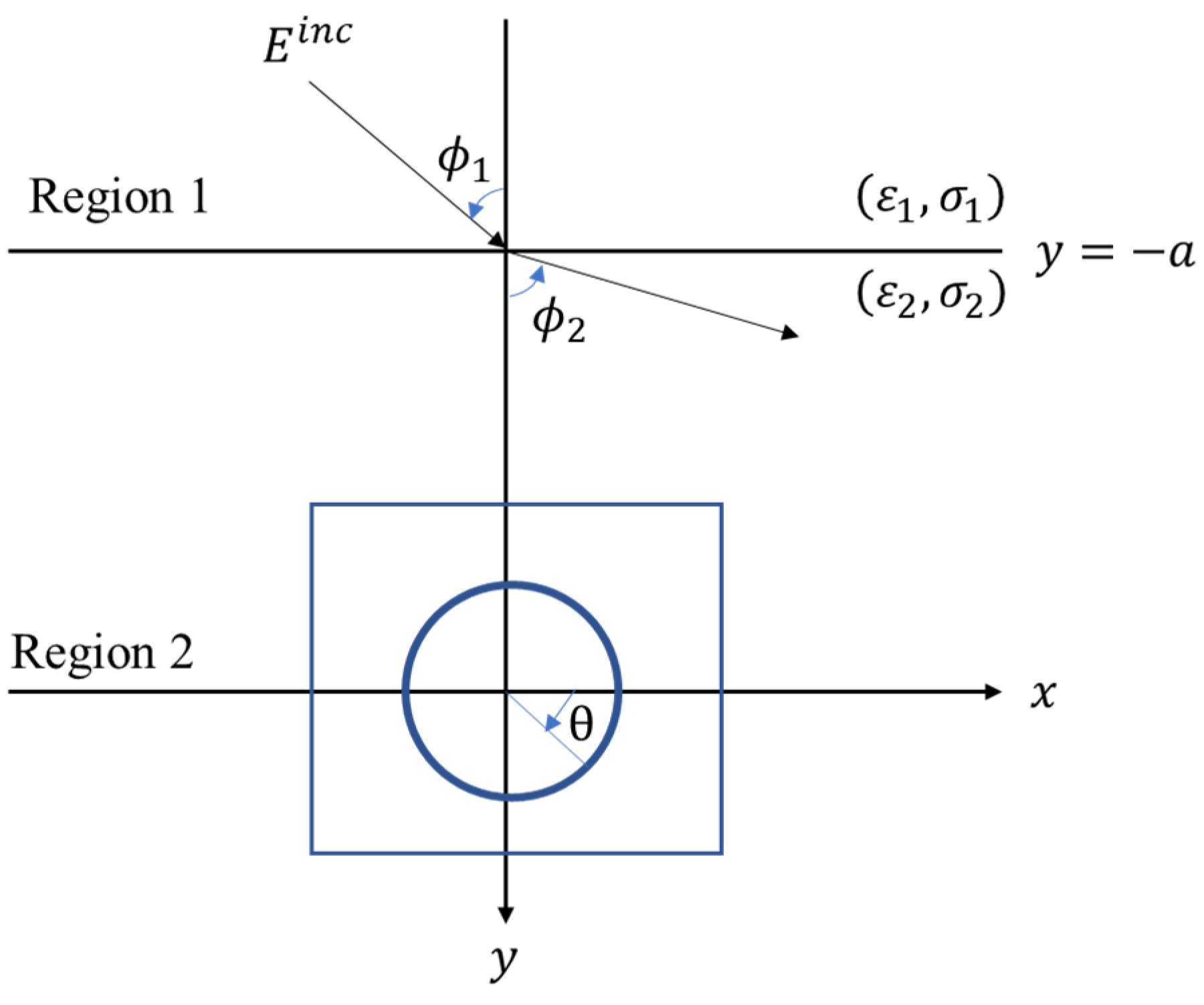
2. Theoretical Formulation

A perfect conductor buried in one half-space is depicted in Figure 1. The permittivity and conductivity in regions 1 and 2 were $\left({\epsilon }_1,{\sigma }_1\right)$ and $\left({\epsilon }_2,{\sigma }_2\right)$, respectively. In each region, the permeability of the free space was set to ${\mu }_0$, that is, only non-magnetic substances were considered. Let the scatterer be a cylindrical conductor extending infinitely in the z-axis. Its cross-sectional area in the $xy$-plane can be expressed by the equation $\rho =F\left(\theta \right)$. The time-varying relation of the incident wave was set to $e^{j\omega t}$ and its incident angle was ${\varnothing }_1$, as depicted in Figure 1.

For simplicity, the TM wave was assumed to be parallel-polarized along the z-axis. $E_i$ can be used to represent the electric field distribution when the conductor is not present, and is expressed as [6]:

$${\overrightarrow{E}}_i\left(\overrightarrow{r}\right)=E_i\left(x,y\right)\widehat{z}$$

(1)

where

$$E_i\left(x,y\right)=\{\begin{array}{cc}{E}_1\left(x,y\right)=e^{-j{k}_1[xsin{\varnothing }_1+\left(y+a\right)cos{\varnothing }_1]}+R_1{e}^{-j{k}_1[xsin{\varnothing }_1-\left(y+a\right)cos{\varnothing }_1]}& ,y\le -a\\ E_2\left(x,y\right)=T{e}^{-j{k}_2[xsin{\varnothing }_2+\left(y+a\right)cos{\varnothing }_2]}& ,y>-a\end{array}$$

(2)

$$R_1=\frac{1-n}{1+n} , T=\frac{2}{1+n} , n=\frac{\cos {\varphi }_2}{\cos {\varphi }_1}\sqrt{\frac{{\epsilon }_2-j{\sigma }_2/\omega }{{\epsilon }_1-j{\sigma }_1/\omega }}$$

(3)

$$k_{1}sin{\varnothing }_1=k_{2}sin{\varnothing }_2$$

(4)

$$k_i^2={\omega }^2{\epsilon }_i{\mu }_0-j\omega {\mu }_0{\sigma }_i,Im\left(k_i\right)\le 0 , i=1,2$$

(5)

$E^{inc}$ is the incident field of the first term of $E_1\left(x,y\right)$. ${\varnothing }_1$ and ${\varnothing }_2$ are the incident and refracted angles in the lossless media regions 1 and 2, respectively. On the contrary, if regions 1 and 2 are the lossy media, ${\varnothing }_1$ and ${\varnothing }_2$ become more complex. The wave form will be very complicated. Its propagation direction is different according to the decay direction. We expressed the overall electric field in the free space as:

$$E\left(x,y\right)=\{\begin{array}{c}{E}_1\left(x,y\right)+E_s\left(x,y\right) ,y\le -a\\ E_2\left(x,y\right)+E_s\left(x,y\right) ,y>-a\end{array}$$

(6)

where $E_s\left(x,y\right)$ is the scatterrd field. Since the size of the interested object in the resonance region is about one wavelength, the scattered field will have a severe diffraction effect. In order to search for the scattered field, Green’s function $G\left(x,y;x’,y’\right)$ must be calculated carefully by first generating a line current source at $\left(x’,y’\right)$ and the corresponding scattered field at $\left(x,y\right)$. By the Fourier transformation technique, $G\left(x,y;x’,y’\right)$ can be expressed as:

$$G\left(x,y;x’,y’\right)=\{\begin{array}{cc}{G}_1\left(x,y;x^{’},y^{’}\right)& ,y\le -a\\ G_2\left(x,y;x^{’},y^{’}\right)=G_f\left(x,y;x^{’},y^{’}\right)+G_s\left(x,y;x^{’},y^{’}\right)& ,y>-a\end{array}$$

(7)

$$G_1\left(x,y;x^{’},y^{’}\right)=\frac{1}{2\pi }{{\displaystyle \int }}_{-\infty }^{\infty }\frac{j}{{\gamma }_1+{\gamma }_2}{e}^{j{\gamma }_1\left(y+a\right)}{e}^{-j{\gamma }_2\left(y’+a\right)}{e}^{-j\alpha \left(x-x^{\prime }\right)}d\alpha$$

(8)

$$G_f\left(x,y;x^{’},y^{’}\right)=\frac{j}{4}{H}_0^{\left(2\right)}\left[k_2\sqrt{{(x-x’)}^2+{(y-y’)}^2}\right]$$

(9)

$$G_s\left(x,y;x^{’},y^{’}\right)=\frac{1}{2\pi }{{\displaystyle \int }}_{-\infty }^{\infty }\frac{j}{2{\gamma }_2}\left(\frac{{\gamma }_2-{\gamma }_1}{{\gamma }_2+{\gamma }_1}\right)e^{-j{\gamma }_2\left(y+2a+y^{\prime }\right)}{e}^{-j\alpha \left(x-x^{\prime }\right)}d\alpha$$

(10)

where ${\gamma }_i^2=k_i^2-{\alpha }^2, Im({\gamma }_i)\le 0, i=1,2$.

Conceptually the scattered field $E_S\left(\mathrm{x},\mathrm{y}\right)$ can be regarded as the surface-induced current $J_s$ on the conductor radiating in half-space. By means of the two-dimensional Green’s function, the scattered field outside the conductor can be expressed as:

$$E_s=\{\begin{array}{c}-{{\displaystyle \int }}_0^{2\pi }{G}_1\left(\stackrel{\rightharpoonup }{r};F\left({\theta }^{\prime }\right),\theta \right)J\left({\theta }^{\prime }\right)d{\theta }^{\prime } , y\le -a\\ -{{\displaystyle \int }}_0^{2\pi }{G}_2\left(\stackrel{\rightharpoonup }{r};F\left({\theta }^{\prime }\right),\theta \right)J\left({\theta }^{\prime }\right)d{\theta }^{\prime } , y>-a\end{array}$$

(11)

where

$$\stackrel{\rightharpoonup }{r}=\left(x,y\right), J\left(\theta \right)=-j\omega {\mu }_0\sqrt{F^2\left(\theta \right)+F^{’2}\left(\theta \right)}{J}_s\left(\theta \right)$$

(12)

The boundary condition for a perfect conductor is that the total electric field in the tangential direction on the surface of the conductor is zero. According to this boundary condition, we can obtain the integral equation of $J\left(\theta \right)$.

$$E_2\left(F\left(\theta \right),\theta \right)={{\displaystyle \int }}_0^{2\pi }{G}_2\left(F\left(\theta \right),\theta ;F\left({\theta }^{\prime }\right),{\theta }^{\prime }\right)J\left({\theta }^{\prime }\right)d{\theta }^{\prime }$$

(13)

The scattered field in region 1 is:

$$E_s\left(x,y\right)=-{{\displaystyle \int }}_0^{2\pi }{G}_1\left(x,y;F\left({\theta }^{\prime }\right),{\theta }^{\prime }\right)J\left({\theta }^{\prime }\right)d{\theta }^{\prime } ,y\le -a$$

(14)

For the direct scattering problem, $E_s$ was calculated from $J\left(\theta \right)$ using the given $F\left(\theta \right)$ shape function in region 1. For inverse problem, any point within the scatterer was presumed. Under this circumstance, $F\left(\theta \right)$ can be expressed as:

$$F\left(\theta \right)={\displaystyle \sum }_{n=0}^{N/2}{B}_n\cos (n\theta )+{\displaystyle \sum }_{n=1}^{N/2}{C}_n\sin (n\theta )$$

(15)

where $B_n$ and $C_n$ denote the parameters to be computed, and N + 1 is an unknown number of the parameters. In the inverse problem, the following objective function, which was minimized using the WOA and SHO, was defined as:

$$OF={\left\{\frac{1}{M_t}{\displaystyle \sum }_{m=1}^{M_t}{\left|E_s^{exp}\left({\overline{r}}_m\right)-E_s^{cal}\left({\overline{r}}_m\right)\right|}^2/{\left|E_s^{exp}\left({\overline{r}}_m\right)\right|}^2\right\}}^{\frac{1}{2}}$$

(16)

where $M_t$ is the measured number. $E_s^{exp}\left({\stackrel{\rightharpoonup }{r}}_m\right)$ and $E_s^{cal}\left({\stackrel{\rightharpoonup }{r}}_m\right)$ are the experimental and computed scattered fields, respectively.

3. Optimization Algorithms

3.1. Whale Optimization Algorithm

The whale optimization algorithm, which simulates the unique hunting behavior of humpback whales, was a conceptual optimization design implemented and proposed by Mirjalili and Lewis in 2016 [21]. According to the research findings, a whale’s brain possesses human-like shuttle cells that are responsible for social, judgment, emotional and other behaviors. This is why, in recent years, people have been curious about these intelligent sea animals. Humpback whales are aggressive hunters. Rather than direct attacks or slapping the seawater with their fins to stun their prey, their mechanism of attack led to the formulation of the bubble-net attacking mechanism that was introduced in the literature [21]. When they hunt in groups, they first dive about 10–15 m in the water, and then form a circular or nine-shaped path underneath the prey and swim quickly around it. They then use their vents to generate spiral air bubbles to crowd the prey together. Eventually, they manage to feed on the prey by following the flow direction of the air bubbles. The basic principle of the WOA is described below.

3.1.1. Encircling the Prey

Instinctively, humpback whales can identify the location of their prey and gather them. While updating their own position, the prey is surrounded. During the search process, a temporary best solution is designated for reference in the algorithm. The current best solution may be the prey location or the position that is the closest to the prey. In the search formula, after defining the initial search position, the position is overridden by the current best position. In other words, the best solution is found by family search.

The position update formula is as follows:

$${\stackrel{\rightharpoonup }{D}}_{we}=|\stackrel{\rightharpoonup }{C}·\stackrel{\rightharpoonup }{Q^{*}}(t)-\stackrel{\rightharpoonup }{Q}(t\left)\right|$$

(17)

$$\stackrel{\rightharpoonup }{Q}\left(t+1\right)=\stackrel{\rightharpoonup }{Q^{*}}\left(t\right)-\stackrel{\rightharpoonup }{A}·{\stackrel{\rightharpoonup }{D}}_{we}$$

(18)

where $\stackrel{\rightharpoonup }{Q^{*}}\left(t\right)$ is the position vector that is the nearest to the prey at the $t$^th iteration (i.e., the current best position vector), and $\stackrel{\rightharpoonup }{Q}\left(t\right)$ is the position vector of the whale at the $t$th iteration. $|\hspace{1em}|$ is the absolute value, and $·$ signifies element-by-element multiplication. The pace coefficient vector $\stackrel{\rightharpoonup }{A}$ and the weight coefficient vector $\stackrel{\rightharpoonup }{C}$ are calculated, respectively, by:

$$\stackrel{\rightharpoonup }{A}=2\stackrel{\rightharpoonup }{ap}·\stackrel{\rightharpoonup }{ran}-\stackrel{\rightharpoonup }{ap}$$

(19)

and

$$\stackrel{\rightharpoonup }{C}=2·\stackrel{\rightharpoonup }{ran}$$

(20)

where $\stackrel{\rightharpoonup }{ap}$ decreases linearly from 2 to 0 during the iterative process and $\stackrel{\rightharpoonup }{ran}$ is a random number vector in [0, 1].

3.1.2. Exploitation Phase

In the development stage, the humpback whale was modeled mathematically according to its bubble-net hunting method and is divided into two models: shrinking encircling mechanism and spiral updating position.

• Shrinking encircling mechanism
  The position update equation of the shrinking encircling mechanism is shown in Equation (17). By decreasing $\stackrel{\rightharpoonup }{ap}$ from 2 to 0 and substituting its value into Equation (18), And when the pace coefficient $\stackrel{\rightharpoonup }{A}$ is in the range of [−1, 1], the search process of the whale algorithm enters the development stage. The current best position $\stackrel{\rightharpoonup }{Q^{*}}\left(t\right)$ is the prey location or the nearest position to the prey. The whale $\stackrel{\rightharpoonup }{Q}\left(t\right)$ then approaches to the best position in order to find the best solution.
• Spiral updating position

When humpback whales hunt, they use their air vents to generate air bubbles. Since they swim rapidly in a nine-shaped or circular path underneath the water level, this spiral-shape air-bubble net traps the prey. Therefore, this algorithm generates a spiral to update the calculated distance between the whale and the current optimal position as follows:

$$\stackrel{\rightharpoonup }{Q}\left(t+1\right)={\stackrel{\rightharpoonup }{D}}_{ws}·e^{bl}·\cos \left(2\pi l\right)+\stackrel{\rightharpoonup }{Q^{*}}\left(t\right)$$

(21)

$${\stackrel{\rightharpoonup }{D}}_{ws}=\left|\stackrel{\rightharpoonup }{Q^{*}}\left(t\right)-\stackrel{\rightharpoonup }{Q}\left(t\right)\right|$$

(22)

${\stackrel{\rightharpoonup }{D}}_{ws}$ denotes the distance between the whale location and the current best position,$b$ is a constant to designate the logarithmic spiral shape, and $l$ is a random number in the range of [−1, 1].

When humpback whales hunt, they swim along the spiral path generated by their air vent bubbles. In order to simulate the behavior of both modes simultaneously, it is assumed that there is a 50% chance that each choosing between the shrinking encircling and the spiral updating mechanisms. The spiral update position during the process is shown below:

$$\stackrel{\rightharpoonup }{Q}\left(t+1\right)=\{\begin{array}{c}\stackrel{\rightharpoonup }{Q^{*}}\left(t\right)-\stackrel{\rightharpoonup }{A}·{\stackrel{\rightharpoonup }{D}}_{we} if p<0.5\\ {\stackrel{\rightharpoonup }{D}}_{ws}·e^{bl}·\cos \left(2\pi l\right)+\stackrel{\rightharpoonup }{Q^{*}}\left(t\right) if p\ge 0.5\end{array}$$

(23)

where $p$ is a random number in the range of [0, 1].

3.1.3. Exploration Phase

During the scouting stage, an individual whale group conducts a random search using the location of any partner as a reference. At this time, the whale algorithm conducts a search in the vicinity of any location to find a better value. If |$\stackrel{\rightharpoonup }{\mathrm{A}}$|$\ge$1, the whale algorithm conducts the exploration phase, forcing the whale to deviate from its original prey target to look for other, more suitable prey. This mechanism enhances the whale’s ability to search and hunt in an entire area.

$${\stackrel{\rightharpoonup }{D}}_{wp}=\left|\stackrel{\rightharpoonup }{C}·{\overrightarrow{Q}}_{rand}\left(t\right)-\stackrel{\rightharpoonup }{Q}\left(t\right)\right|$$

(24)

$$\stackrel{\rightharpoonup }{Q}\left(t+1\right)={\overrightarrow{Q}}_{rand}\left(t\right)-\stackrel{\rightharpoonup }{A}·{\stackrel{\rightharpoonup }{D}}_{wp}$$

(25)

where ${\overrightarrow{Q}}_{rand}$ is an arbitrary position vector.

Note that |$\stackrel{\rightharpoonup }{\mathrm{A}}$|$\ge$1 means that all elements of $\stackrel{\rightharpoonup }{\mathrm{A}}$ are greater or equal to 1. In summary, a random number $p$ and $\stackrel{\rightharpoonup }{\mathrm{A}}$ are generated using Equation (19). When $p\ge 0.5$, the location is updated via Equation (21), whereas, if $p<0.5$, the location is updated by Equation (25) when |$\stackrel{\rightharpoonup }{\mathrm{A}}$|$\ge$1 and by Equation (18) when |$\stackrel{\rightharpoonup }{\mathrm{A}}$|$<$ 1. The objective function value is computed to obtain the best solution whenever there is one. The process is executed iteratively until the stopping criteria are met.

3.2. Spotted Hyena Optimizer

The spotted hyena optimizer (SHO), which simulates the hunting behavior of spotted hyenas, is an optimal algorithm proposed by Dhiman and Kaur in 2017 [26]. Hyenas are a very intelligent species. They use multiple senses to identify relatives or other individuals as well as to rank them within the same species by trusting the higher priority group first. The predation mechanism for the spotted hyena is composed of three processes: encircling, hunting and attacking the prey. The basic principle of the spotted hyena algorithm is described as follows:

3.2.1. Encircling the Prey

Spotted hyenas locate their prey and then surround it. The mathematical model for this behavior is expressed as:

$${\stackrel{\rightharpoonup }{D}}_{he}=\left|\stackrel{\rightharpoonup }{B}·{\stackrel{\rightharpoonup }{P}}_p\left(t\right)-\stackrel{\rightharpoonup }{P}\left(t\right)\right|$$

(26)

$$\stackrel{\rightharpoonup }{B}=2·\stackrel{\rightharpoonup }{R{d}_1}$$

(27)

where ${\stackrel{\rightharpoonup }{D}}_{he}$ is the distance between the prey and spotted hyena, $t$ is the current iterations, ${\stackrel{\rightharpoonup }{P}}_p$ is the prey position vector,$\stackrel{\rightharpoonup }{P}\left(t\right)$ is the spotted hyena position vector, and $B$ is the sway factor. $\stackrel{\rightharpoonup }{R{d}_1}$ is a random number vector in the range of [0, 1].

Next, the location of each spotted hyena is updated to:

$$\stackrel{\rightharpoonup }{P}\left(t+1\right)={\stackrel{\rightharpoonup }{P}}_p\left(t\right)-\stackrel{\rightharpoonup }{L}·{\stackrel{\rightharpoonup }{D}}_{he}$$

(28)

$$\stackrel{\rightharpoonup }{L}=2\stackrel{\rightharpoonup }{h}·\stackrel{\rightharpoonup }{R{d}_2}-\stackrel{\rightharpoonup }{h}$$

(29)

$$\stackrel{\rightharpoonup }{h}=5-\left(Iteration\times \left(5/Ma{x}_{Iteration}\right)\right)$$

(30)

where $\stackrel{\rightharpoonup }{L}$ is the convergence factor. $\stackrel{\rightharpoonup }{R{d}_2}$ denotes a random number vector in the range of [0, 1]. $\stackrel{\rightharpoonup }{h}$ decreases linearly from 5 to 0. Max iteration is the maximum iteration number.

3.2.2. Hunting

As mentioned earlier, the community of spotted hyenas usually hunts its prey using a trusted species network and, then, identifies its location, as mathematically specified in Equation (31):

$${\stackrel{\rightharpoonup }{D}}_{hh}=\left|\stackrel{\rightharpoonup }{B}·{\stackrel{\rightharpoonup }{P}}_h-{\stackrel{\rightharpoonup }{P}}_k\right|$$

(31)

$${\stackrel{\rightharpoonup }{P}}_k={\stackrel{\rightharpoonup }{P}}_h-\stackrel{\rightharpoonup }{L}·{\stackrel{\rightharpoonup }{D}}_{hh}$$

(32)

$${\stackrel{\rightharpoonup }{C}}_h={\stackrel{\rightharpoonup }{P}}_k+{\stackrel{\rightharpoonup }{P}}_{k+1}+\cdots +{\stackrel{\rightharpoonup }{P}}_{k+\mathrm{n}}$$

(33)

where ${\stackrel{\rightharpoonup }{P}}_h$ is the position of the first best spotted hyena. ${\stackrel{\rightharpoonup }{P}}_k$ is the position of other spotted hyenas. ${\stackrel{\rightharpoonup }{C}}_h\mathrm{is}\mathrm{the}\mathrm{cluster}\mathrm{of}\mathrm{the}N\mathrm{best}\mathrm{solutions}.N$ denotes the number of spotted hyenas.

$$N=coun{t}_{nos}\left({\stackrel{\rightharpoonup }{P}}_h,{\stackrel{\rightharpoonup }{P}}_{h+1},\cdots ,\left({\stackrel{\rightharpoonup }{P}}_h+\stackrel{\rightharpoonup }{RM}\right)\right)$$

(34)

where $\stackrel{\rightharpoonup }{RM}$ is a random vector in the range of [0.5, 1]. After adding $RM$, the number of feasible solutions $nos$ is defined and all candidate solutions are calculated.

3.2.3. Attacking Prey (Exploitation)

Spotted hyenas start to attack their prey in the last stage of the hunt, when the coefficient $\left|\stackrel{\rightharpoonup }{L}\right|<1$. Its location is revised by using the average of the current optimal solution set. The formula for attacking the prey is expressed as:

$$\stackrel{\rightharpoonup }{P}\left(t+1\right)=\frac{{\stackrel{\rightharpoonup }{C}}_h}{N}$$

(35)

where $\stackrel{\rightharpoonup }{P}\left(t+1\right)$ presents the best solution and updates the positions of other spotted hyena according to the position of the best spotted hyena.

In brief, Equations (33) and (34) are used to calculate the best solution group and Equation (35) is used to update the position of each search agent. Next, the objective function is calculated to update the position of the search agent if a better solution is found. Lastly, the spotted hyenas group is updated through the new objective function value of the search agent. Again, the iteration is terminated as soon as the stopping criteria are reached.

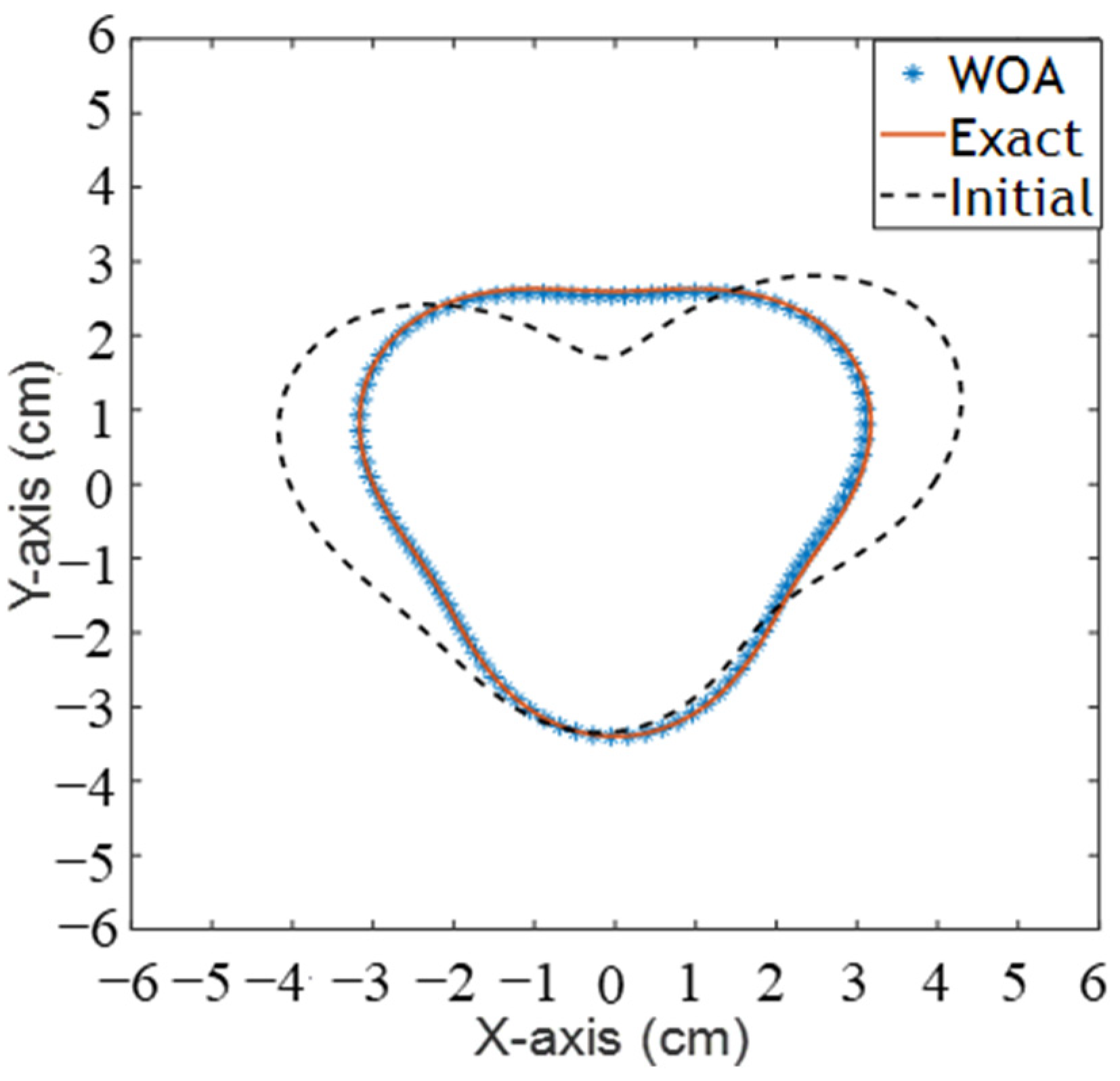
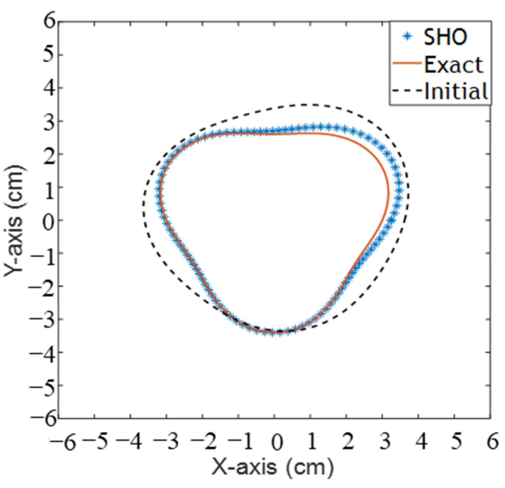
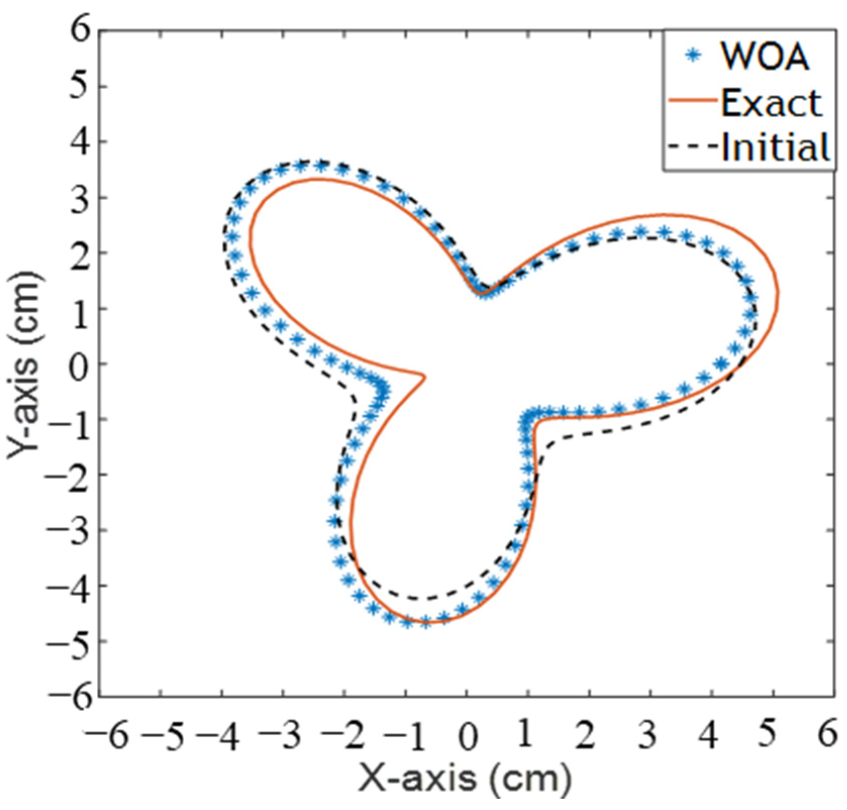
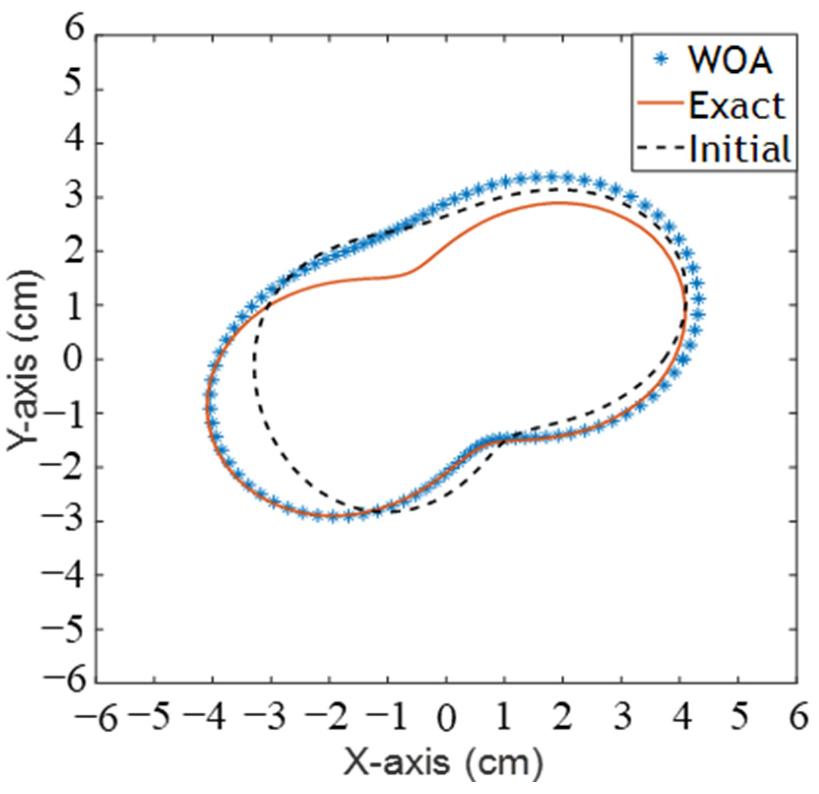
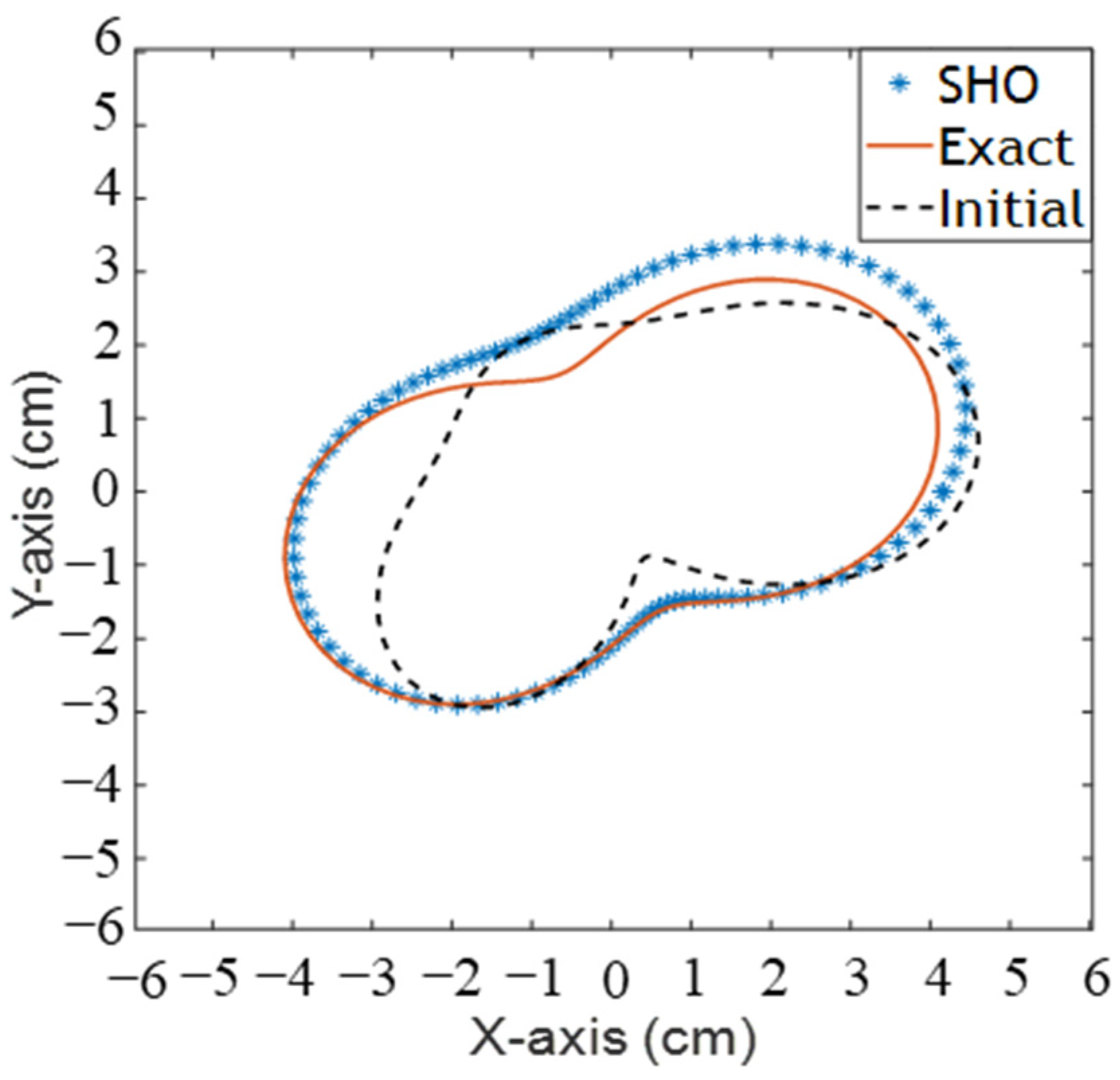
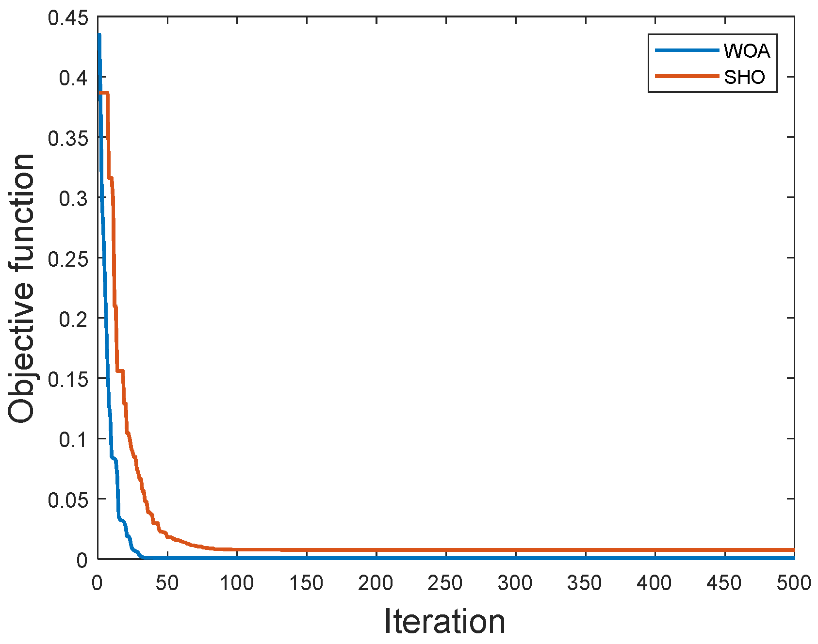
4. Numerical Results

We first considered a perfect conductor concealed in the half-space. Figure 1 shows that an amplitude 1 electromagnetic wave is incident on region 1 with a frequency of 3 GHz and a wavelength of 10 cm. $\mathrm{The}\mathrm{buried}\mathrm{depth}\mathrm{at} y=-a=-10\mathrm{cm}$. The background substance in region 1 is air, i.e., ${\mathsf{\epsilon }}_1={\mathsf{\epsilon }}_0$ and ${\sigma }_1=0$. The background substance in region 2 is the soil with ${\mathsf{\epsilon }}_2=2.56 {\mathsf{\epsilon }}_0$ and ${\sigma }_2=0$. In the numerical simulation, we used three different directions of incident waves ($\varnothing =-{60}^{°},0^{°}\mathrm{and}{60}^{°}$) to show the buried object. There were 20 equally spaced measurement points from $x=-10 \mathrm{cm}$ to $x=10 \mathrm{cm}$ to receive the scattered field along the media $y=-10 \mathrm{cm}$. We aimed to utilize the received scattered field collected from various incident angles for reshaping the object. To investigate the effects of noise, we added a quantity of (b + cj) to each complex scattered field, where b and c are independent random numbers with a uniform distribution over 0 to the noise level times the R.M.S value of the scattered field. The numerical results were obtained with a noise level of 1%.

In this research, three inverse scattering examples were investigated using the WOA and SHO. The shape function $F\left(\theta \right)\mathrm{was}\mathrm{chosen}\mathrm{to}\mathrm{be}\left(3+0.4sin3\theta \right) \mathrm{cm}$ in the first example. This scatterer was set to a smoother shape. The respective reconstructed shape functions by the WOA and SHO were good, as shown in Figure 2 and Figure 3. Comparing Figure 2 and Figure 3, it can be seen that, although the initial guess of the WOA was poor, it still converged to a better result. It is clear that the backside of the object was not reconstructed well by the SHO. The shape function discrepancies DISR were defined as:

$$DISR={\left\{\frac{1}{N^{\prime }}{\displaystyle \sum }_{i=1}^{N^{\prime }}{\left[F^{cal}\left({\theta }_i\right)-F\left({\theta }_i\right)\right]}^2/F^2\left({\theta }_i\right)\right\}}^{\frac{1}{2}}$$

(36)

where $N’$ was set to 100. The DISR was about 1.5% and 4.7% using the WOA and SHO, respectively. From the numerical results, it can be seen that the reconstruction of the WOA is better than that of the SHO.

The shape function was defined as $F\left(\theta \right)=\left(3+0.5cos\theta +1cos3\theta +1.5sin3\theta \right) \mathrm{cm}$ in the second example. The buried object was set to a three-petal shape for example 2. From Figure 4 and Figure 5, it can be observed that the shape functions reconstructed by the WOA and SHO were not bad, although there was some discrepancy on the upper part. This is due to the fact that the backside of the object was more difficult to rebuild. Note that the upper part of the object in the figure corresponds to the back side of the buried object. The DISR was about 11.6% and 14.0% by the WOA and SHO, respectively. From Figure 4 and Figure 5, it can be seen that the initial guess values of the two algorithms were similar. However, the reconstruction results show that the WOA is better than the SHO.

We defined the shape function to be $F\left(\theta \right)=\left(3+0.9cos3\theta +0.9sin2\theta \right)\mathrm{cm}$ in the last example. The buried object was set to be a peanut shape. Figure 6 and Figure 7 show the shape functions reconstructed by the WOA and SHO for the best members, respectively. It can be seen that the initial shape of the WOA is better than that of the SHO for this example. It was found that the shape functions reconstructed by the WOA and SHO had some discrepancies in the upper part, especially on the right-hand side. The DISR was about 12.3% and 14.6% by the WOA and SHO, respectively. From the numerical results, it can be seen that the WOA and SHO were less accurate in reconstructing the concave surface on the back of the peanut. Apparently, the reconstruction performance for the WOA overwhelms that of the SHO.

Regarding the computational resources for the two algorithms shown in

Table 1. Computational resources for the two algorithms.

	Method	SHO	WOA
Resources
Memory		2G	2G
Time		843 sec	845 sec

, the SHO took 843 s with CPU 3.8-GHz Intel Core i7 Processor and 32-GB RAM for example 1, while the WOA took 845 s. Although the WOA took a little more time, it was able to reconstruct better results, as shown in

Table 2. DISR for the SHO and WOA.

	Method	SHO	WOA
Example
Example 1		4.7%	1.5%
Example 2		14.0%	11.6%
Example 3		14.6%	12.3%

. The convergence of the algorithms for each iteration is shown in Figure 8.

5. Conclusions

The two-dimensional inverse scattering processes for a perfect conductor buried in a half-space via the WOA and SHO algorithms were compared in this paper. By irradiating a TM-polarized wave with a 1% noise interference, the two algorithms were employed in the frequency domain for image reconstruction. TM waves were irradiated from the other half-space to a perfect conductor with an unknown shape buried in one half-space. The scattered field measured outside the conductor surface with the boundary condition was used to reconstruct the object via the WOA and SHO algorithms. The inverse scattering problem was solved to obtain an optimized solution resulting from the implementation of the WOA and SHO. According to the numerical simulation, the reconstruction performance was more favorable to the WOA than the SHO using the same parameters. This is due to the random generation of initial guesses for both optimization methods. However, the WOA had a better search ability than the SHO in a wide area. In our future work, we will consider combining the WOA and SHO with AI techniques for electromagnetic imaging.

References

1. Lewis, R.M. Physical optics inverse diffraction. IEEE Trans. Antennas Propag. 1969, 17, 308–314. [Google Scholar] [CrossRef]
2. Bojarski, N.N. A survey of the physical optics inverse scattering identity. IEEE Trans. Antennas Propag. 1982, 30, 980–989. [Google Scholar] [CrossRef]
3. Chu, T.H.; Farhat, N.H. Polarization effects in microwave diversity imaging of perfectly conducting cylinders. IEEE Trans. Antennas Propagar. 1989, 37, 235–244. [Google Scholar] [CrossRef]
4. Ge, D.B. A study of Lewis method for target-shape reconstruction. Inverse Probl. 1990, 6, 363–370. [Google Scholar] [CrossRef]
5. Chu, T.H.; Lin, D.B. Microwave diversity imaging of perfectly conducting objects in the near-field region. IEEE Trans. Microw. Theory Tech. 1991, 39, 480–487. [Google Scholar]
6. Harrmgton, R.F. Field Computation by Moment Method; Wiley-IEEE Press: New York, MA, USA, 1968. [Google Scholar]
7. Roger, A. Newton-Kantorovitch algorithm applied to an electromagnetic inverse problem. IEEE Trans. Antennas Propag. 1981, 29, 232–238. [Google Scholar] [CrossRef]
8. Tobocman, W. Inverse acoustic wave scattering in two dimensions from impenetrable targets. Inverse Probl. 1989, 5, 1131–1144. [Google Scholar] [CrossRef]
9. Chiu, C.C.; Kiang, Y.M. Electromagnetic imaging for an imperfectly conducting cylinder. IEEE Trans. Microw. Theory Tech. 1991, 39, 1631–1639. [Google Scholar]
10. Otto, G.P.; Chew, W.C. Microwave Inverse Scattering-Local Shape Function Imaging for Improved Resolution of Strong Scatters. IEEE Trans. Microw. Theory Tech. 1994, 42, 137–141. [Google Scholar] [CrossRef]
11. Colton, D.; Monk, P. Anovel method for solving the inverse scattering problem for time-harmonic acoustic waves in the resonance region D. SIAMJ. Appl. Math. 1986, 46, 506–523. [Google Scholar] [CrossRef]
12. Kirsch, A.; Kress, R.; Monk, P.; Zinn, A. Two methods for solving the inverse acoustic scattering problem. Inverse Probl. 1988, 4, 749–770. [Google Scholar] [CrossRef]
13. Hettlich, F. Two methods for solving an inverse conductive scattering problem. Inverse Probl. 1994, 10, 375–385. [Google Scholar] [CrossRef]
14. Caorsi, S.; Gragnani, G.L.; Pastorina, M. An approach to microwave imaging using a multiview moment method solution for a two-dimensional infinite cylinder. IEEE Trans. Microw. Theory Tech. 1991, 39, 1062–1067. [Google Scholar] [CrossRef]
15. Zheng, X.; Hu, B. Analysis of Incident Field Polarization of A DDA Based Inverse Scattering Imaging Algorithm. In Proceedings of the 2021 13th International Symposium on Antennas, Propagation and EM Theory (ISAPE), Zhuhai, China, 1–4 December 2021. [Google Scholar]
16. Holland, J.H. Adaptation in Natural and Artificial System; University of Michigan Press: Ann Arbor, MI, USA, 1975. [Google Scholar]
17. Chiu, C.C.; Yen, C.Y.; Lee, G.Z. Dielectric Objects Reconstruction by Combining Subspace-based Algorithm and Randomly Global Optimization Algorithm. J. Electromagn. Waves Appl. 2018, 32, 77–91. [Google Scholar] [CrossRef]
18. Chien, W.; Chiu, C.C.; Chen, P.H.; Jiang, H.; Chan, S.J. Imaging of Rough Surfaces by Near-Field Measurement. Sens. Mater. 2021, 33, 2333–2344. [Google Scholar] [CrossRef]
19. Mirjalili, S.; Lewis, A. The Whale Optimization Algorithm. Adv. Eng. Softw. 2016, 95, 51–67. [Google Scholar] [CrossRef]
20. Ling, Y.; Zhou, Y.; Luo, Q. Levy Flight Trajectory-Based Whale Optimization Algorithm for Global Optimization. IEEE Access Brows. J. Mag. 2017, 5, 6168–6186. [Google Scholar] [CrossRef]
21. Yan, Z.H.; Sha, J.X.; Liu, B.; Lu, J. An Ameliorative Whale Optimization Algorithm for Multi—Objective Optimal Allocation of Water Resources in Handan, China. Water 2018, 10, 87. [Google Scholar] [CrossRef]
22. Lee, K.C.; Lu, P.T. Application of Whale Optimization Algorithm to Inverse Scattering of an Imperfect Conductor with Corners. Int. J. Antennas Propag. 2020, 2020, 8205797. [Google Scholar] [CrossRef]
23. Chakraborty, S.; Saha, A.K.; Sharma, S.; Mirjalili, S.; Chakraborty, R. A novel enhanced whale optimization algorithm for global optimization. Comput. Ind. Eng. 2021, 153, 107086. [Google Scholar] [CrossRef]
24. Lin, X.; Yu, X.; Li, W. A heuristic whale optimization algorithm with niching strategy for global multi-dimensional engineering optimization. Comput. Ind. Eng. 2022, 171, 108361. [Google Scholar] [CrossRef]
25. Dhiman, G.; Kaura, V. Spotted hyena optimizer: A novel bio-inspired based metaheuristic technique for engineering applications. Adv. Eng. Softw. 2017, 114, 48–70. [Google Scholar] [CrossRef]
26. Dhiman, G.; Kaur, A. Spotted Hyena Optimizer for Solving Engineering Design Problems. In Proceedings of the 2017 International Conference on Machine Learning and Data Science (MLDS), Noida, India, 14–15 December 2017; pp. 114–119. [Google Scholar]
27. Sukpancharoen, S. Application of Spotted Hyena Optimizer in Cogeneration Power Plant on Single and Multiple-Objective. In Proceedings of the 2021 IEEE 11th Annual Computing and Communication Workshop and Conference (CCWC), Las Vegas, NV, USA, 27–30 January 2021; pp. 0001–0005. [Google Scholar]
28. Yi, Z.; Sun, X.B.; Li, Z.; Yang, S.X.; Sun, Y.F. Research on Three-Phase Unbalanced Commutation Strategy Based on the Spotted Hyena Optimizer Algorithm. Complexity 2022, 2022, 1–10. [Google Scholar]
29. Vega, E.; Soto, R.; Crawford, B.; Peña, J.; Contreras, P.; Castrob, C. Predicting population size and termination criteria in metaheuristics: A case study based on spotted hyena optimizer and crow search algorithm. Appl. Soft Comput. 2022, 128, 109513. [Google Scholar] [CrossRef]
Figure 1. Schematic diagram of a two-dimensional perfect conductor in half-space.
Applsci 13 05857 g001
Figure 2. WOA reconstruction of the shape function for example 1.
Applsci 13 05857 g002
Figure 3. SHO reconstruction of the shape function for example 1.
Applsci 13 05857 g003
Figure 4. WOA reconstruction of the shape function for example 2.
Applsci 13 05857 g004
Figure 5. SHO reconstruction of the shape function for example 2.
Applsci 13 05857 g005
Figure 6. WOA reconstruction of the shape function for example 3.
Applsci 13 05857 g006
Figure 7. SHO reconstruction of the shape function for example 3.
Applsci 13 05857 g007
Figure 8. The root-mean-square error of the scattered field as a function of iteration by the SHO and WOA for example 1.
Applsci 13 05857 g008