A Combination of Feature Selection and Random Forest Techniques to Solve a Problem Related to Blast-Induced Ground Vibration

 , , and
Abstract
:1. Introduction
2. Methods
2.1. Input Selection Technique
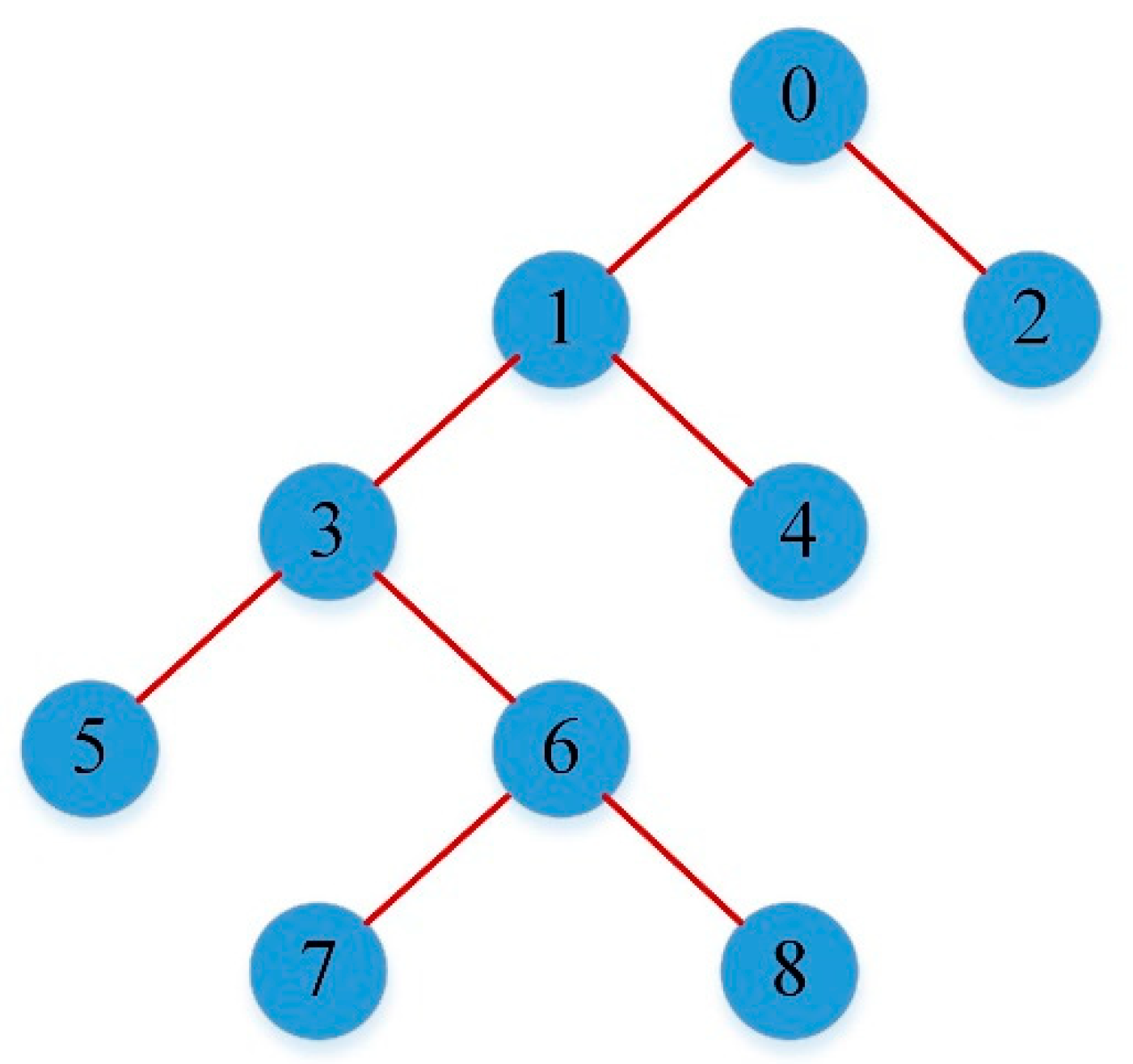
2.2. Decision Trees
2.3. Artificial Neural Network
2.4. Support Vector Machine
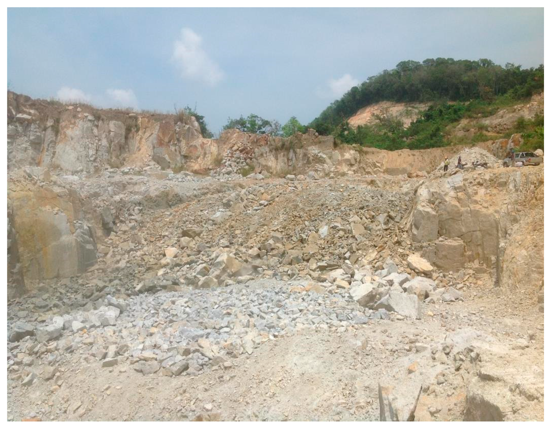
2.5. Case Study and Data Collection
3. Results
3.1. Input Selection Using FS Technique
3.2. Development of ML Models
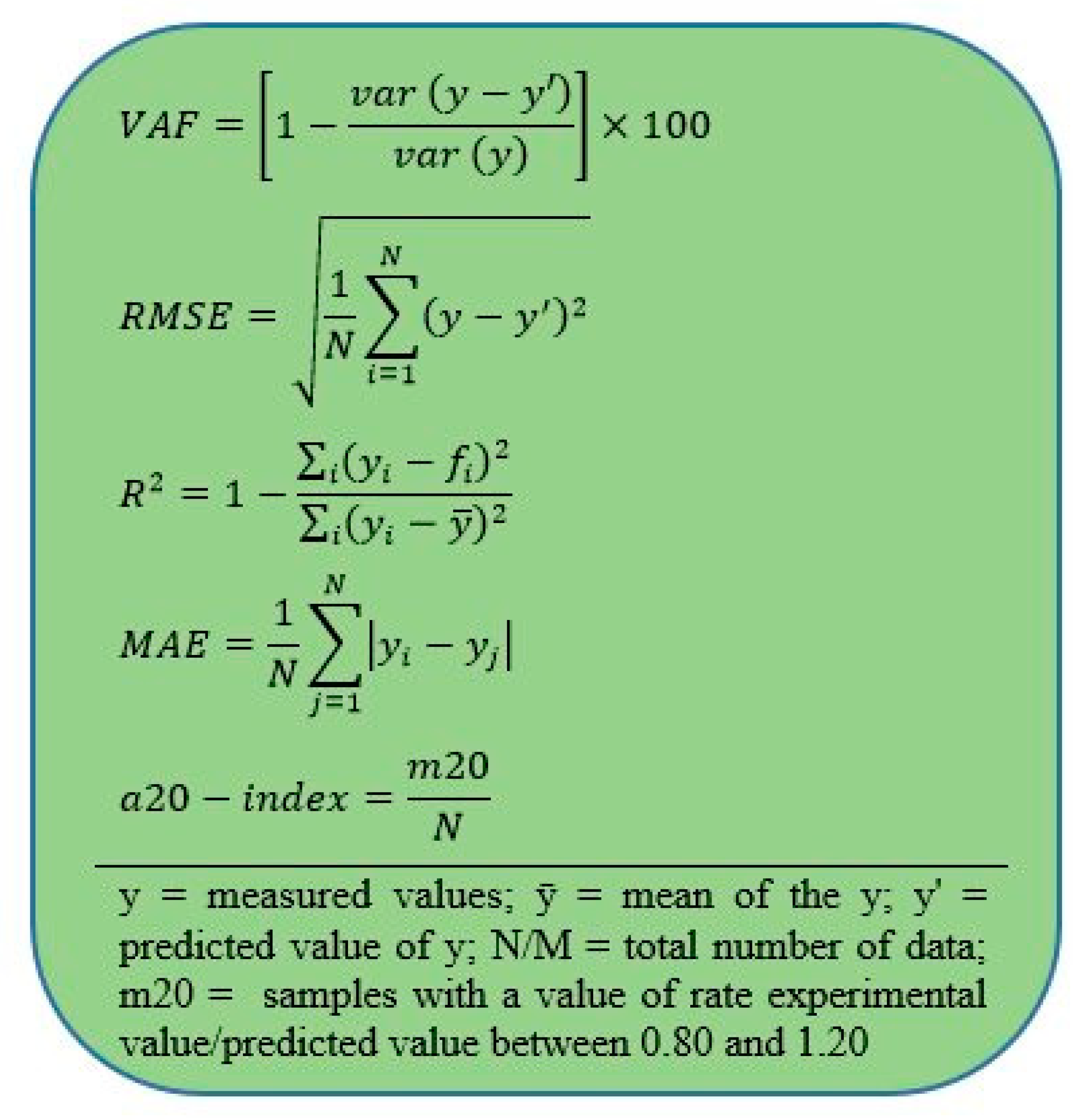
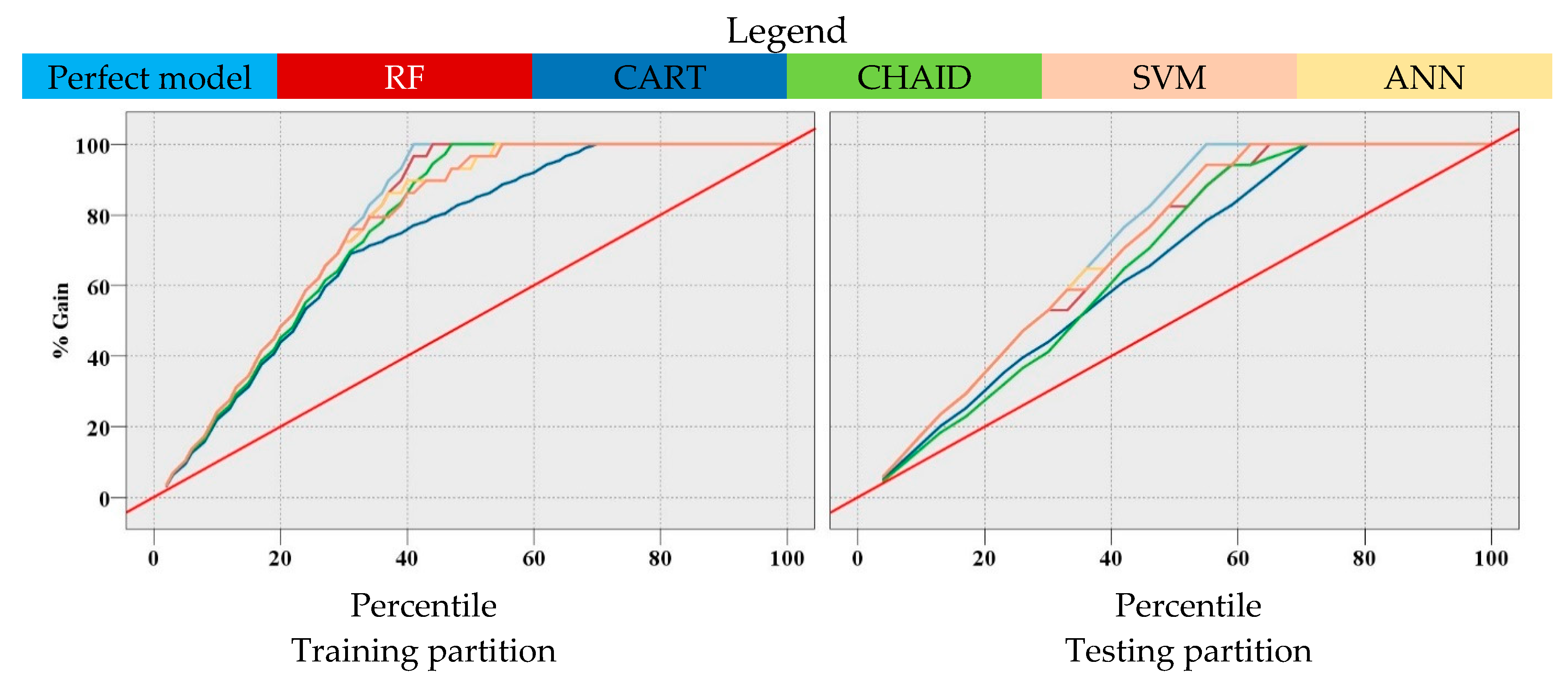
3.3. Assessment of the Proposed Models
4. Summary and Conclusions
Author Contributions
Funding
Conflicts of Interest
Abbreviations
| ANFIS | Adaptive neuro-fuzzy inference system |
| ANN | Artificial neural network |
| CHAID | Chi-squared automatic interaction detection |
| CART | Classification and regression trees |
| R2 | Coefficient of determination |
| FS | Feature selection |
| FIS | Fuzzy inference system |
| GEP | Gene expression programming |
| GA | Genetic algorithm |
| GP | Genetic programming |
| ICA | Imperialism competitive algorithm |
| ML | Machine learning |
| MAE | Mean absolute error |
| MLP | Multilayer perception |
| PSO | Particle swarm optimization |
| PPV | Peak particle velocity |
| QUEST | Quick, unbiased, efficient, and statistical tree |
| RBF | Radial basis function |
| RF | Random forest |
| RMSE | Root mean square error |
| SVM | Support vector machine |
| VAF | Variance accounted for |
References
- Khandelwal, M.; Kumar, D.L.; Yellishetty, M. Application of soft computing to predict blast-induced ground vibration. Eng. Comput. 2011, 27, 117–125. [Google Scholar] [CrossRef]
- Ebrahimi, E.; Monjezi, M.; Khalesi, M.R.; Armaghani, D.J. Prediction and optimization of back-break and rock fragmentation using an artificial neural network and a bee colony algorithm. Bull. Eng. Geol. Environ. 2016, 75, 27–36. [Google Scholar] [CrossRef]
- Dindarloo, S.R. Prediction of blast-induced ground vibrations via genetic programming. Int. J. Min. Sci. Technol. 2015, 25, 1011–1015. [Google Scholar] [CrossRef]
- Armaghani, D.J.; Hajihassani, M.; Mohamad, E.T.; Marto, A.; Noorani, S.A. Blasting-induced flyrock and ground vibration prediction through an expert artificial neural network based on particle swarm optimization. Arab. J. Geosci. 2014, 7, 5383–5396. [Google Scholar] [CrossRef]
- Hajihassani, M.; Jahed Armaghani, D.; Sohaei, H.; Tonnizam Mohamad, E.; Marto, A. Prediction of airblast-overpressure induced by blasting using a hybrid artificial neural network and particle swarm optimization. Appl. Acoust. 2014, 80, 57–67. [Google Scholar] [CrossRef]
- Armaghani, D.J.; Hajihassani, M.; Sohaei, H.; Mohamad, E.T.; Marto, A.; Motaghedi, H.; Moghaddam, M.R. Neuro-fuzzy technique to predict air-overpressure induced by blasting. Arab. J. Geosci. 2015, 8, 10937–10950. [Google Scholar] [CrossRef]
- Tonnizam Mohamad, E.; Hajihassani, M.; Jahed Armaghani, D.; Marto, A. Simulation of blasting-induced air overpressure by means of Artificial Neural Networks. Int. Rev. Model. Simul. 2012, 5, 2501–2506. [Google Scholar]
- Mohamad, E.T.; Armaghani, D.J.; Noorani, S.A.; Saad, R.; Alvi, S.V.; Abad, N.K. Prediction of flyrock in boulder blasting using artificial neural network. Electron. J. Geotech. Eng. 2012, 17, 2585–2595. [Google Scholar]
- Khandelwal, M.; Singh, T.N. Prediction of blast-induced ground vibration using artificial neural network. Int. J. Rock Mech. Min. Sci. 2009, 46, 1214–1222. [Google Scholar] [CrossRef]
- Hasanipanah, M.; Bakhshandeh Amnieh, H.; Khamesi, H.; Jahed Armaghani, D.; Bagheri Golzar, S.; Shahnazar, A. Prediction of an environmental issue of mine blasting: An imperialistic competitive algorithm-based fuzzy system. Int. J. Environ. Sci. Technol. 2018, 15, 551–560. [Google Scholar] [CrossRef]
- Monjezi, M.; Ahmadi, M.; Sheikhan, M.; Bahrami, A.; Salimi, A.R. Predicting blast-induced ground vibration using various types of neural networks. Soil Dyn. Earthq. Eng. 2010, 30, 1233–1236. [Google Scholar] [CrossRef]
- Armaghani, D.J.; Momeni, E.; Abad, S.V.A.N.K.; Khandelwal, M. Feasibility of ANFIS model for prediction of ground vibrations resulting from quarry blasting. Environ. Earth Sci. 2015, 74, 2845–2860. [Google Scholar] [CrossRef] [Green Version]
- Singh, T.N.; Singh, V. An intelligent approach to prediction and control ground vibration in mines. Geotech. Geol. Eng. 2005, 23, 249–262. [Google Scholar] [CrossRef]
- Toraño, J.; Ramírez-Oyanguren, P.; Rodríguez, R.; Diego, I. Analysis of the environmental effects of ground vibrations produced by blasting in quarries. Int. J. Min. Reclam. Environ. 2006, 20, 249–266. [Google Scholar] [CrossRef]
- Ozer, U.; Kahriman, A.; Aksoy, M.; Adiguzel, D.; Karadogan, A. The analysis of ground vibrations induced by bench blasting at Akyol quarry and practical blasting charts. Environ. Geol. 2008, 54, 737–743. [Google Scholar] [CrossRef]
- Faramarzi, F.; Farsangi, M.A.E.; Mansouri, H. Simultaneous investigation of blast induced ground vibration and airblast effects on safety level of structures and human in surface blasting. Int. J. Min. Sci. Technol. 2014, 24, 663–669. [Google Scholar] [CrossRef]
- Duvall, W.I.; Petkof, B. Spherical Propagation of Explosion-Generated Strain Pulses in Rock; USBM: Washington, DC, USA, 1959.
- Dowding, C.H. Suggested Method for Blast Vibration Monitoring. Int. J. Rock Mech. Min. Sci. Geomech. Abstr. 1992, 29, 145–156. [Google Scholar] [CrossRef]
- Indian Standard. Criteria for Safety and Design of Structures Subjected to under Ground Blast; No 15-6922; ISI: Karnataka, India, 1973.
- Kahriman, A. Analysis of ground vibrations caused by bench blasting at can open-pit lignite mine in Turkey. Environ. Geol. 2002, 41, 653–661. [Google Scholar] [CrossRef]
- Ambraseys, N.N.; Hendron, A.J. Dynamic Behaviour of Rock Masses; John Wiley & Sons: Hoboken, NJ, USA, 1968. [Google Scholar]
- Davies, B.; Farmer, I.W.; Attewell, P.B. Ground vibration from shallow sub-surface blasts. Engineer 1964, 217, 5644. [Google Scholar]
- Langefors, U.; Kihlstrom, B. The Modern Technique of Rock Blasting; Wiley: New York, NY, USA, 1963. [Google Scholar]
- Roy, P. Putting ground vibration predictions into practice. Colliery Guard. 1993, 241, 63–67. [Google Scholar]
- Khandelwal, M.; Singh, T.N. Evaluation of blast-induced ground vibration predictors. Soil Dyn. Earthq. Eng. 2007, 27, 116–125. [Google Scholar] [CrossRef]
- Verma, A.K.; Singh, T.N. Intelligent systems for ground vibration measurement: A comparative study. Eng. Comput. 2011, 27, 225–233. [Google Scholar] [CrossRef]
- Verma, A.K.; Singh, T.N. A neuro-fuzzy approach for prediction of longitudinal wave velocity. Neural Comput. Appl. 2013, 22, 1685–1693. [Google Scholar] [CrossRef]
- Hudaverdi, T. Application of multivariate analysis for prediction of blast-induced ground vibrations. Soil Dyn. Earthq. Eng. 2012, 43, 300–308. [Google Scholar] [CrossRef]
- Hajihassani, M.; Jahed Armaghani, D.; Marto, A.; Tonnizam Mohamad, E. Ground vibration prediction in quarry blasting through an artificial neural network optimized by imperialist competitive algorithm. Bull. Eng. Geol. Environ. 2014, 74, 873–886. [Google Scholar] [CrossRef]
- Monjezi, M.; Baghestani, M.; Shirani Faradonbeh, R.; Pourghasemi Saghand, M.; Jahed Armaghani, D. Modification and prediction of blast-induced ground vibrations based on both empirical and computational techniques. Eng. Comput. 2016, 32, 717–728. [Google Scholar] [CrossRef]
- Mohamed, M.T. Performance of fuzzy logic and artificial neural network in prediction of ground and air vibrations. Int. J. Rock Mech. Min. Sci. 2011, 48, 845. [Google Scholar] [CrossRef]
- Xu, H.; Zhou, J.; Asteris, P.G.; Jahed Armaghani, D.; Tahir, M.M. Supervised Machine Learning Techniques to the Prediction of Tunnel Boring Machine Penetration Rate. Appl. Sci. 2019, 9, 3715. [Google Scholar] [CrossRef] [Green Version]
- Apostolopoulou, M.; Armaghani, D.J.; Bakolas, A.; Douvika, M.G.; Moropoulou, A.; Asteris, P.G. Compressive strength of natural hydraulic lime mortars using soft computing techniques. Procedia Struct. Integr. 2019, 17, 914–923. [Google Scholar] [CrossRef]
- Gordan, B.; Jahed Armaghani, D.; Hajihassani, M.; Monjezi, M. Prediction of seismic slope stability through combination of particle swarm optimization and neural network. Eng. Comput. 2016, 32, 85–97. [Google Scholar] [CrossRef]
- Zhou, J.; Aghili, N.; Ghaleini, E.N.; Bui, D.T.; Tahir, M.M.; Koopialipoor, M. A Monte Carlo simulation approach for effective assessment of flyrock based on intelligent system of neural network. Eng. Comput. 2019. [Google Scholar] [CrossRef]
- Zhou, J.; Koopialipoor, M.; Murlidhar, B.R.; Fatemi, S.A.; Tahir, M.M.; Armaghani, D.J.; Li, C. Use of Intelligent Methods to Design Effective Pattern Parameters of Mine Blasting to Minimize Flyrock Distance. Nat. Resour. Res. 2019. [Google Scholar] [CrossRef]
- Koopialipoor, M.; Murlidhar, B.R.; Hedayat, A.; Armaghani, D.J.; Gordan, B.; Mohamad, E.T. The use of new intelligent techniques in designing retaining walls. Eng. Comput. 2019, 36, 283–294. [Google Scholar] [CrossRef]
- Guo, H.; Zhou, J.; Koopialipoor, M.; Armaghani, D.J.; Tahir, M.M. Deep neural network and whale optimization algorithm to assess flyrock induced by blasting. Eng. Comput. 2019. [Google Scholar] [CrossRef]
- Armaghani, D.J.; Koopialipoor, M.; Marto, A.; Yagiz, S. Application of several optimization techniques for estimating TBM advance rate in granitic rocks. J. Rock Mech. Geotech. Eng. 2019, 11, 779–789. [Google Scholar] [CrossRef]
- Harandizadeh, H.; Armaghani, D.J.; Khari, M. A new development of ANFIS–GMDH optimized by PSO to predict pile bearing capacity based on experimental datasets. Eng. Comput. 2019. [Google Scholar] [CrossRef]
- Khari, M.; Dehghanbandaki, A.; Motamedi, S.; Armaghani, D.J. Computational estimation of lateral pile displacement in layered sand using experimental data. Measurement 2019, 146, 110–118. [Google Scholar] [CrossRef]
- Shao, Z.; Armaghani, D.J.; Bejarbaneh, B.Y.; Mu’azu, M.A.; Mohamad, E.T. Estimating the Friction Angle of Black Shale Core Specimens with Hybrid-ANN Approaches. Measurement 2019, 145, 744–755. [Google Scholar] [CrossRef]
- Chen, W.; Sarir, P.; Bui, X.-N.; Nguyen, H.; Tahir, M.M.; Armaghani, D.J. Neuro-genetic, neuro-imperialism and genetic programing models in predicting ultimate bearing capacity of pile. Eng. Comput. 2019. [Google Scholar] [CrossRef]
- Hajihassani, M.; Abdullah, S.S.; Asteris, P.G.; Armaghani, D.J. A Gene Expression Programming Model for Predicting Tunnel Convergence. Appl. Sci. 2019, 9, 4650. [Google Scholar] [CrossRef] [Green Version]
- Zhou, J.; Li, X.; Mitri, H.S. Evaluation method of rockburst: State-of-the-art literature review. Tunn. Undergr. Space Technol. 2018, 81, 632–659. [Google Scholar] [CrossRef]
- Zhou, J.; Li, E.; Yang, S.; Wang, M.; Shi, X.; Yao, S.; Mitri, H.S. Slope stability prediction for circular mode failure using gradient boosting machine approach based on an updated database of case histories. Saf. Sci. 2019, 118, 505–518. [Google Scholar] [CrossRef]
- Wang, M.; Shi, X.; Zhou, J.; Qiu, X. Multi-planar detection optimization algorithm for the interval charging structure of large-diameter longhole blasting design based on rock fragmentation aspects. Eng. Optim. 2018, 50, 2177–2191. [Google Scholar] [CrossRef]
- Zhou, J.; Li, E.; Wei, H.; Li, C.; Qiao, Q.; Armaghani, D.J. Random Forests and Cubist Algorithms for Predicting Shear Strengths of Rockfill Materials. Appl. Sci. 2019, 9, 1621. [Google Scholar] [CrossRef] [Green Version]
- Zhou, J.; Li, E.; Wang, M.; Chen, X.; Shi, X.; Jiang, L. Feasibility of Stochastic Gradient Boosting Approach for Evaluating Seismic Liquefaction Potential Based on SPT and CPT Case Histories. J. Perform. Constr. Facil. 2019, 33, 4019024. [Google Scholar] [CrossRef]
- Asteris, P.G.; Mokos, V.G. Concrete compressive strength using artificial neural networks. Neural Comput. Appl. 2019. [Google Scholar] [CrossRef]
- Huang, L.; Asteris, P.G.; Koopialipoor, M.; Armaghani, D.J.; Tahir, M.M. Invasive Weed Optimization Technique-Based ANN to the Prediction of Rock Tensile Strength. Appl. Sci. 2019, 9, 5372. [Google Scholar] [CrossRef] [Green Version]
- Apostolopoulour, M.; Douvika, M.G.; Kanellopoulos, I.N.; Moropoulou, A.; Asteris, P.G. Prediction of Compressive Strength of Mortars using Artificial Neural Networks. In Proceedings of the 1st International Conference TMM_CH, Transdisciplinary Multispectral Modelling and Cooperation for the Preservation of Cultural Heritage, Athens, Greece, 10–13 October 2018; pp. 10–13. [Google Scholar]
- Zhou, J.; Li, X.; Shi, X. Long-term prediction model of rockburst in underground openings using heuristic algorithms and support vector machines. Saf. Sci. 2012, 50, 629–644. [Google Scholar] [CrossRef]
- Zhou, J.; Li, X.B.; Mitri, H.S. Classification of rockburst in underground projects: Comparison of ten supervised learning methods. J. Comput. Civ. Eng. 2016, 30, 04016003. [Google Scholar] [CrossRef]
- Sarir, P.; Chen, J.; Asteris, P.G.; Armaghani, D.J.; Tahir, M.M. Developing GEP tree-based, neuro-swarm, and whale optimization models for evaluation of bearing capacity of concrete-filled steel tube columns. Eng. Comput. 2019. [Google Scholar] [CrossRef]
- Yang, H.Q.; Xing, S.G.; Wang, Q.; Li, Z. Model test on the entrainment phenomenon and energy conversion mechanism of flow-like landslides. Eng. Geol. 2018, 239, 119–125. [Google Scholar] [CrossRef]
- Yang, H.Q.; Zeng, Y.Y.; Lan, Y.F.; Zhou, X.P. Analysis of the excavation damaged zone around a tunnel accounting for geostress and unloading. Int. J. Rock Mech. Min. Sci. 2014, 69, 59–66. [Google Scholar] [CrossRef]
- Liu, B.; Yang, H.; Karekal, S. Effect of Water Content on Argillization of Mudstone During the Tunnelling process. Rock Mech. Rock Eng. 2019. [Google Scholar] [CrossRef]
- Yang, H.; Liu, J.; Liu, B. Investigation on the cracking character of jointed rock mass beneath TBM disc cutter. Rock Mech. Rock Eng. 2018, 51, 1263–1277. [Google Scholar] [CrossRef]
- Yang, H.Q.; Li, Z.; Jie, T.Q.; Zhang, Z.Q. Effects of joints on the cutting behavior of disc cutter running on the jointed rock mass. Tunn. Undergr. Space Technol. 2018, 81, 112–120. [Google Scholar] [CrossRef]
- Armaghani, D.J.; Hatzigeorgiou, G.D.; Karamani, C.; Skentou, A.; Zoumpoulaki, I.; Asteris, P.G. Soft computing-based techniques for concrete beams shear strength. Procedia Struct. Integr. 2019, 17, 924–933. [Google Scholar] [CrossRef]
- Chen, H.; Asteris, P.G.; Jahed Armaghani, D.; Gordan, B.; Pham, B.T. Assessing Dynamic Conditions of the Retaining Wall: Developing Two Hybrid Intelligent Models. Appl. Sci. 2019, 9, 1042. [Google Scholar] [CrossRef] [Green Version]
- Asteris, P.G.; Nikoo, M. Artificial bee colony-based neural network for the prediction of the fundamental period of infilled frame structures. Neural Comput. Appl. 2019, 31, 4837–4847. [Google Scholar] [CrossRef]
- Asteris, P.G.; Nozhati, S.; Nikoo, M.; Cavaleri, L.; Nikoo, M. Krill herd algorithm-based neural network in structural seismic reliability evaluation. Mech. Adv. Mater. Struct. 2019, 26, 1146–1153. [Google Scholar] [CrossRef]
- Asteris, P.; Roussis, P.; Douvika, M. Feed-forward neural network prediction of the mechanical properties of sandcrete materials. Sensors 2017, 17, 1344. [Google Scholar] [CrossRef] [Green Version]
- Cavaleri, L.; Asteris, P.G.; Psyllaki, P.P.; Douvika, M.G.; Skentou, A.D.; Vaxevanidis, N.M. Prediction of Surface Treatment Effects on the Tribological Performance of Tool Steels Using Artificial Neural Networks. Appl. Sci. 2019, 9, 2788. [Google Scholar] [CrossRef] [Green Version]
- Khandelwal, M.; Singh, T.N. Prediction of blast induced ground vibrations and frequency in opencast mine: A neural network approach. J. Sound Vib. 2006, 289, 711–725. [Google Scholar] [CrossRef]
- Monjezi, M.; Ghafurikalajahi, M.; Bahrami, A. Prediction of blast-induced ground vibration using artificial neural networks. Tunn. Undergr. Space Technol. 2011, 26, 46–50. [Google Scholar] [CrossRef]
- Fişne, A.; Kuzu, C.; Hüdaverdi, T. Prediction of environmental impacts of quarry blasting operation using fuzzy logic. Environ. Monit. Assess. 2011, 174, 461–470. [Google Scholar] [CrossRef]
- Iphar, M.; Yavuz, M.; Ak, H. Prediction of ground vibrations resulting from the blasting operations in an open-pit mine by adaptive neuro-fuzzy inference system. Environ. Geol. 2008, 56, 97–107. [Google Scholar] [CrossRef]
- Mohamadnejad, M.; Gholami, R.; Ataei, M. Comparison of intelligence science techniques and empirical methods for prediction of blasting vibrations. Tunn. Undergr. Space Technol. 2012, 28, 238–244. [Google Scholar] [CrossRef]
- Li, D.T.; Yan, J.L.; Zhang, L. Prediction of blast-induced ground vibration using support vector machine by tunnel excavation. Appl. Mech. Mater. 2012, 170, 1414–1418. [Google Scholar] [CrossRef]
- Ghasemi, E.; Ataei, M.; Hashemolhosseini, H. Development of a fuzzy model for predicting ground vibration caused by rock blasting in surface mining. J. Vib. Control 2013, 19, 755–770. [Google Scholar] [CrossRef]
- Monjezi, M.; Hasanipanah, M.; Khandelwal, M. Evaluation and prediction of blast-induced ground vibration at Shur River Dam, Iran, by artificial neural network. Neural Comput. Appl. 2013, 22, 1637–1643. [Google Scholar] [CrossRef]
- Hasanipanah, M.; Monjezi, M.; Shahnazar, A.; Armaghani, D.J.; Farazmand, A. Feasibility of indirect determination of blast induced ground vibration based on support vector machine. Measurement 2015, 75, 289–297. [Google Scholar] [CrossRef]
- Dindarloo, S.R. Peak particle velocity prediction using support vector machines: A surface blasting case study. J. S. Afr. Inst. Min. Metall. 2015, 115, 637–643. [Google Scholar] [CrossRef]
- Hajihassani, M.; Jahed Armaghani, D.; Monjezi, M.; Mohamad, E.T.; Marto, A. Blast-induced air and ground vibration prediction: A particle swarm optimization-based artificial neural network approach. Environ. Earth Sci. 2015, 74, 2799–2817. [Google Scholar] [CrossRef]
- Hasanipanah, M.; Faradonbeh, R.S.; Amnieh, H.B.; Armaghani, D.J.; Monjezi, M. Forecasting blast-induced ground vibration developing a CART model. Eng. Comput. 2017, 33, 307–316. [Google Scholar] [CrossRef]
- Armaghani, D.J.; Hasanipanah, M.; Amnieh, H.B.; Mohamad, E.T. Feasibility of ICA in approximating ground vibration resulting from mine blasting. Neural Comput. Appl. 2018, 29, 457–465. [Google Scholar] [CrossRef]
- Shirani Faradonbeh, R.; Jahed Armaghani, D.; Abd Majid, M.Z.; MD Tahir, M.; Ramesh Murlidhar, B.; Monjezi, M.; Wong, H.M. Prediction of ground vibration due to quarry blasting based on gene expression programming: A new model for peak particle velocity prediction. Int. J. Environ. Sci. Technol. 2016, 13, 1453–1464. [Google Scholar] [CrossRef] [Green Version]
- Shahnazar, A.; Nikafshan Rad, H.; Hasanipanah, M.; Tahir, M.M.; Jahed Armaghani, D.; Ghoroqi, M. A new developed approach for the prediction of ground vibration using a hybrid PSO-optimized ANFIS-based model. Environ. Earth Sci. 2017, 76, 527. [Google Scholar] [CrossRef]
- Ghoraba, S.; Monjezi, M.; Talebi, N.; Armaghani, D.J.; Moghaddam, M.R. Estimation of ground vibration produced by blasting operations through intelligent and empirical models. Environ. Earth Sci. 2016, 75, 1137. [Google Scholar] [CrossRef]
- Breiman, L.; Friedman, J.; Olshen, R.; Stone, C. Classification and regression trees. Wadsworth Int. Group 1984, 37, 237–251. [Google Scholar]
- Kass, G.V. An exploratory technique for investigating large quantities of categorical data. J. R. Stat. Soc. Ser. C Appl. Stat. 1980, 29, 119–127. [Google Scholar] [CrossRef]
- Brown, G. Ensemble Learning. In Encyclopedia of Machine Learning; Springer: Boston, MA, USA, 2010; pp. 312–320. [Google Scholar]
- Breiman, L. Random forests. Mach. Learn. 2001, 45, 5–32. [Google Scholar] [CrossRef] [Green Version]
- Cybenko, G. Approximation by superpositions of a sigmoidal function. Math. Control. Signals Syst. 1989, 2, 303–314. [Google Scholar] [CrossRef]
- Vapnik, V.; Vapnik, V. Statistical Learning Theory; Wiley: New York, NY, USA, 1998; pp. 156–160. [Google Scholar]
- Kavzoglu, T.; Sahin, E.K.; Colkesen, I. Landslide susceptibility mapping using GIS-based multi-criteria decision analysis, support vector machines, and logistic regression. Landslides 2014, 11, 425–439. [Google Scholar] [CrossRef]
- Hasanipanah, M.; Shahnazar, A.; Bakhshandeh Amnieh, H.; Jahed Armaghani, D. Prediction of air-overpressure caused by mine blasting using a new hybrid PSO–SVR model. Eng. Comput. 2017, 33, 23–31. [Google Scholar] [CrossRef]
- Cortes, C.; Vapnik, V. Support-vector networks. Mach. Learn. 1995, 20, 273–297. [Google Scholar] [CrossRef]
- Hong, H.; Pradhan, B.; Bui, D.T.; Xu, C.; Youssef, A.M.; Chen, W. Comparison of four kernel functions used in support vector machines for landslide susceptibility mapping: A case study at Suichuan area (China). Geomat. Nat. Hazards Risk 2017, 8, 544–569. [Google Scholar] [CrossRef]
- Kalantar, B.; Pradhan, B.; Naghibi, S.A.; Motevalli, A.; Mansor, S. Assessment of the effects of training data selection on the landslide susceptibility mapping: A comparison between support vector machine (SVM), logistic regression (LR) and artificial neural networks (ANN). Geomat. Nat. Hazards Risk 2018, 9, 49–69. [Google Scholar] [CrossRef]
- Toghroli, A.; Mohammadhassani, M.; Suhatril, M.; Shariati, M.; Ibrahim, Z. Prediction of shear capacity of channel shear connectors using the ANFIS model. Steel Compos. Struct. 2014, 17, 623–639. [Google Scholar] [CrossRef]
- Asteris, P.G.; Apostolopoulou, M.; Skentou, A.D.; Moropoulou, A. Application of artificial neural networks for the prediction of the compressive strength of cement-based mortars. Comput. Concr. 2019, 24, 329–345. [Google Scholar]
- Khari, M.; Armaghani, D.J.; Dehghanbanadaki, A. Prediction of Lateral Deflection of Small-Scale Piles Using Hybrid PSO–ANN Model. Arab. J. Sci. Eng. 2019. [Google Scholar] [CrossRef]
- Asteris, P.G.; Tsaris, A.K.; Cavaleri, L.; Repapis, C.C.; Papalou, A.; Di Trapani, F.; Karypidis, D.F. Prediction of the fundamental period of infilled RC frame structures using artificial neural networks. Comput. Intell. Neurosci. 2016, 2016, 20. [Google Scholar] [CrossRef] [Green Version]
- Bui, X.-N.; Jaroonpattanapong, P.; Nguyen, H.; Tran, Q.-H.; Long, N.Q. A novel Hybrid Model for predicting Blast-induced Ground Vibration Based on k-nearest neighbors and particle Swarm optimization. Sci. Rep. 2019, 9, 1–14. [Google Scholar] [CrossRef] [Green Version]
- Kuncheva, L.I.; Whitaker, C.J. Measures of diversity in classifier ensembles and their relationship with the ensemble accuracy. Mach. Learn. 2003, 51, 181–207. [Google Scholar] [CrossRef]
- Guyon, I.; Elisseeff, A. An introduction to variable and feature selection. J. Mach. Learn. Res. 2003, 3, 1157–1182. [Google Scholar]
- Cortés, G.; Benitez, M.C.; García, L.; Álvarez, I.; Ibanez, J.M. A comparative study of dimensionality reduction algorithms applied to volcano-seismic signals. IEEE J. Sel. Top. Appl. Earth Obs. Remote Sens. 2015, 9, 253–263. [Google Scholar] [CrossRef]


| Study | Technique | No. of Input Variables | No. of Datasets |
|---|---|---|---|
| Iphar et al. [70] | ANFIS | 2 | 44 |
| Monjezi et al. [68] | ANN | 4 | 182 |
| Khandelwal et al. [1] | ANN | 2 | 130 |
| Mohamed [31] | ANN, FIS | 2 | 162 |
| Fisne et al. [69] | FIS | 2 | 33 |
| Li et al. [72] | SVM | 2 | 32 |
| Mohamadnejad et al. [71] | SVM, ANN | 2 | 37 |
| Ghasemi et al. [73] | FIS | 6 | 120 |
| Monjezi et al. [74] | ANN | 3 | 20 |
| Jahed Armaghani et al. [4] | PSO–ANN | 9 | 44 |
| Hajihassani et al. [29] | ICA–ANN | 7 | 95 |
| Hasanipanah et al. [75] | SVM | 2 | 80 |
| Dindarloo [76] | SVM | 12 | 100 |
| Hajihassani et al. [77] | PSO–ANN | 8 | 88 |
| Jahed Armaghani et al. [12] | ANFIS | 2 | 109 |
| Hasanipanah et al. [78] | CART | 2 | 86 |
| Jahed Armaghani et al. [79] | ICA | 2 | 73 |
| Faradonbeh et al. [80] | GEP | 6 | 102 |
| Shahnazar et al. [81] | PSO–ANFIS | 2 | 81 |
| Ghoraba et al. [82] | ANN, ANFIS | 2 | 115 |
| Screening Rules | Cut-Off * |
|---|---|
| Maximum percentage of missing values | 70 |
| Maximum percentage of records in a single category | 90 |
| Maximum number of categories as a percentage of records | 95 |
| Minimum coefficient of variation | 0.1 |
| Minimum standards deviation | 0.0 |
| Value for important variables | 0.95 |
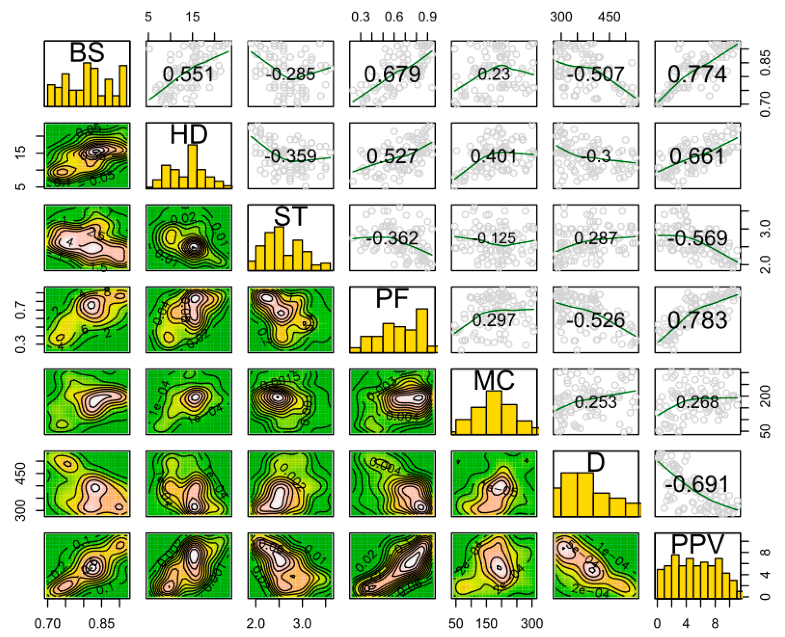
| Parameter | Burden to Spacing Ratio | Distance from the Blast Face | Stemming Length | Maximum Charge Per Delay | Powder Factor | Hole Depth | Peak Particle Velocity |
|---|---|---|---|---|---|---|---|
| Symbol | BS | D | ST | MC | PF | HD | PPV |
| Unit | - | m | m | kg | kg/m3 | m | mm/s |
| Maximum | 0.92 | 531 | 3.6 | 305.6 | 0.94 | 23.2 | 11.05 |
| Minimum | 0.7 | 285 | 1.9 | 45.8 | 0.23 | 5.2 | 0.13 |
| Mean | 0.82 | 379.5 | 2.63 | 179.6 | 0.65 | 14.1 | 5.34 |
| Type | Input | Input | Input | Input | Input | Input | Output |
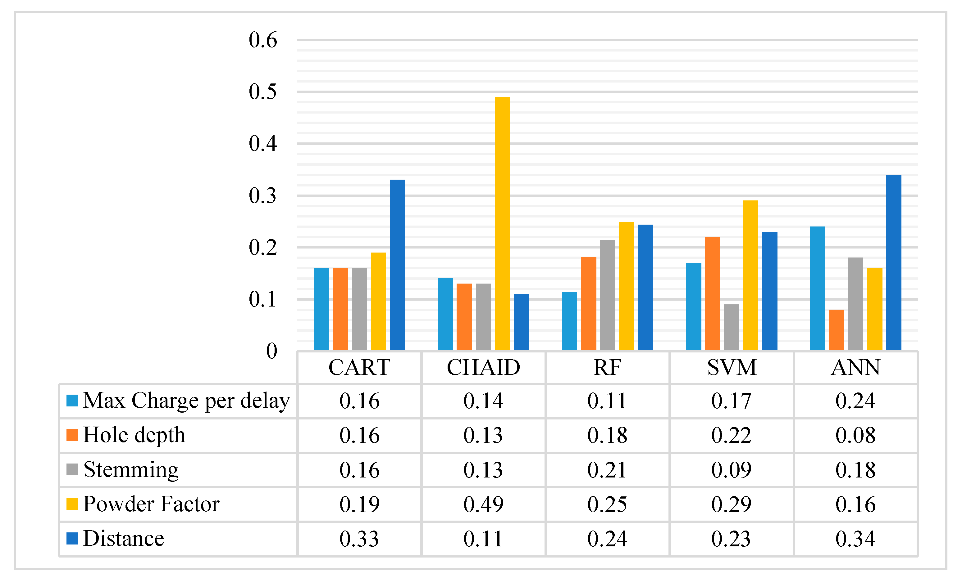
| Input | PF | D | HD | ST | MC |
|---|---|---|---|---|---|
| Importance value | 1.00 | 1.00 | 1.00 | 1.00 | 0.98 |
| R2 * | RMSE ** | VAF *** | MAE **** | a20-Index ***** | Total Rank | Final Rank | |||||||
|---|---|---|---|---|---|---|---|---|---|---|---|---|---|
| Model | Dataset | Value | Rank | Value | Rank | Value | Rank | Value | Rank | Value | Rank | ||
| RF | TR | 0.94 | 5 | 0.77 | 5 | 92.97 | 5 | 0.62 | 4 | 0.73 | 4 | 23 | 41 |
| TE | 0.83 | 3 | 1.46 | 4 | 82.17 | 3 | 1.19 | 3 | 0.55 | 5 | 18 | ||
| CART | TR | 0.67 | 1 | 1.67 | 1 | 67.03 | 1 | 1.32 | 1 | 0.44 | 1 | 5 | 10 |
| TE | 0.56 | 1 | 2.39 | 1 | 54.6 | 1 | 1.84 | 1 | 0.42 | 1 | 5 | ||
| CHAID | TR | 0.91 | 4 | 0.86 | 4 | 91.3 | 4 | 0.54 | 5 | 0.77 | 5 | 22 | 32 |
| TE | 0.68 | 2 | 1.9 | 2 | 67.79 | 2 | 1.47 | 2 | 0.43 | 2 | 10 | ||
| ANN | TR | 0.89 | 3 | 0.96 | 3 | 89.14 | 3 | 0.75 | 3 | 0.66 | 2 | 14 | 35 |
| TE | 0.84 | 4 | 1.41 | 5 | 83.71 | 4 | 1.13 | 5 | 0.52 | 3 | 21 | ||
| SVM | TR | 0.88 | 2 | 1.02 | 2 | 88.48 | 2 | 0.77 | 2 | 0.67 | 3 | 11 | 32 |
| TE | 0.85 | 5 | 1.5 | 3 | 84.54 | 5 | 1.17 | 4 | 0.53 | 4 | 21 | ||
© 2020 by the authors. Licensee MDPI, Basel, Switzerland. This article is an open access article distributed under the terms and conditions of the Creative Commons Attribution (CC BY) license (http://creativecommons.org/licenses/by/4.0/).
Share and Cite
Zhang, H.; Zhou, J.; Jahed Armaghani, D.; Tahir, M.M.; Pham, B.T.; Huynh, V.V. A Combination of Feature Selection and Random Forest Techniques to Solve a Problem Related to Blast-Induced Ground Vibration. Appl. Sci. 2020, 10, 869. https://doi.org/10.3390/app10030869
Zhang H, Zhou J, Jahed Armaghani D, Tahir MM, Pham BT, Huynh VV. A Combination of Feature Selection and Random Forest Techniques to Solve a Problem Related to Blast-Induced Ground Vibration. Applied Sciences. 2020; 10(3):869. https://doi.org/10.3390/app10030869
Chicago/Turabian StyleZhang, Hong, Jian Zhou, Danial Jahed Armaghani, M. M. Tahir, Binh Thai Pham, and Van Van Huynh. 2020. "A Combination of Feature Selection and Random Forest Techniques to Solve a Problem Related to Blast-Induced Ground Vibration" Applied Sciences 10, no. 3: 869. https://doi.org/10.3390/app10030869