Article

Magnetic Anomalies of the Tyrrhenian Sea Revisited: A Processing Workflow for Enhancing the Resolution of Aeromagnetic Data

by
Giovanni Florio
1,*,
Salvatore Passaro
2,
Giovanni de Alteriis
2 and
Federico Cella
3
1
Department of Earth Sciences, Environment and Resources, University of Naples Federico II, 80126 Naples, Italy
2
CNR-ISMAR, Istituto di Scienze Marine, 80133 Naples, Italy
3
Section of Geology, School of Sciences and Technologies, University of Camerino, 62032 Camerino, Italy
*
Author to whom correspondence should be addressed.
Geosciences 2022, 12(10), 377; https://doi.org/10.3390/geosciences12100377
Submission received: 16 July 2022 / Revised: 22 September 2022 / Accepted: 23 September 2022 / Published: 10 October 2022

Abstract

:
We propose a processing workflow to enhance the information content of aeromagnetic data. Our workflow is based on the downward continuation and subsequent L-transform of magnetic data. This workflow returns a map showing single highs, which correspond to the location of magnetic bodies, and does not need any a priori information about the source magnetization. We validated our workflow using the aeromagnetic anomalies of the Tyrrhenian Sea (Italy), by a comparison of the reprocessed aeromagnetic anomalies with high-resolution shipborne magnetic data in three selected areas. Through this comparison, we show that the proposed processing workflow of aeromagnetic data leads to more accurate interpretative results. Our results indicate that, in areas where higher resolution data are lacking, the reprocessing of aeromagnetic data according to our workflow may be as decisive as to suggest changes to their previous interpretations or, at least, useful for highlighting areas of special interest, deserving to be magnetically explored by a dedicated high-resolution shipborne survey.

1. Introduction

The acquisition and analysis of magnetic data represents a fast and non-invasive way for obtaining information about the Earth’s interior at various scales, from depths of a few centimeters to tens of kilometers. Magnetic surveys can be planned for obtaining answers to a wide range of geological and engineering problems. Typical geological applications include the determination of the depth to basement in basin areas [1], of the presence of intrusions [2], of the position of faults and lineaments [3] or of mineral deposits [4], the study of volcanoes [5], of the hydrothermal alteration at depth [6], the geological mapping [7], or the depth to the bottom of the magnetized crust [8], which is associated with the Curie temperature.
This brief list of possible applications clarifies the potential importance of these kinds of data from a scientific as well as economic point of view. Magnetic data can be rapidly collected from different moving platforms, such as satellites, planes, ships, aerial [9] or submarine drones (ROV; [10]) and, of course, magnetometers can be carried by hand while walking in local ground surveys. These different platforms imply differences in the resolution of the acquired data and in the uniformity of magnetic field sampling in an area. The resolution with which a geological structure is seen in a magnetic map is dictated by the distance to the target and the separation of the survey lines. Thus, ground or shipborne surveys can have a high resolution but may suffer from the presence of obstacles preventing data acquisition in some areas. Aeromagnetic or drone-borne magnetic data have lower resolutions, but conduct uniform sampling across the area of interest.
Many hundreds of thousands of linear kilometers of aeromagnetic data have been acquired over wide regions or continents from planes flying at altitudes typically ranging from 500 to 2500 m above ground, allowing the study of magnetic anomalies generated by geological targets at a resolution of several kilometers. Generally, the magnetic surveys are performed at a constant altitude, although sometimes a “draped-survey” is chosen, flying at an approximately constant height above the topography.
However, more accurate, better positioned, and more detailed data are often needed for thorough assessments of the local geological structures. Nevertheless, the cost of new higher resolution surveys may not always be affordable; in these cases, the only possibility to obtain geologic insights from magnetic data is to analyze old, higher altitude, low-resolution regional aeromagnetic data. When analyzing aeromagnetic datasets, it is essential to be able to extract as much information as possible, somehow enhancing their resolution. The processing of aeromagnetic data can take advantage of many specific filters and transformations which improve the readability of magnetic maps (e.g., reduction to the pole filter [11]) as well as to enhance the high-wavenumber part of the spectrum (e.g., vertical differentiation [12]), enabling better separation of the effects of nearby sources.
In this paper, we demonstrate the potentialities of a processing workflow based on published filtering tools, aiming to enhance the information content of aeromagnetic data. After its description, we present its application to the aeromagnetic data in selected areas of the Tyrrhenian Sea (Italy). We evaluated the obtained results by comparing the enhanced aeromagnetic data with the magnetic anomaly maps relative to three local, high-resolution shipborne surveys. This comparison demonstrated that by following our procedure, it is possible to obtain, from high-altitude data, a transformed magnetic field with an information content similar to that of marine datasets and useful for improving the interpretation of local structures.

2. Materials and Methods

The process of enhancing aeromagnetic data implies, in their spectral representation, a relative amplification of high wavenumbers. The practical effect of this amplification is a reduction in the mutual interference and of coalescence effects, so that the individual contributions to the magnetic field generated by nearby sources are more visible and separated than in the original data. Another useful enhancement of the aeromagnetic anomalies would be to simplify their shape, reducing the bipolarity, typical of magnetic anomalies at mid-latitudes, to a single magnetic high or low located in correspondence to their source. This simplification is required not only for removing the ambiguity about the source position, but also for reducing the interference and the complicated patterns it can create. Definitely, even bipolarity removal can increase the resolution of a magnetic anomaly map.
The data resolution is primarily dependent on the acquisition altitude; therefore, a filtering method highly appropriate for enhancing aeromagnetic data is the analytical downward continuation [11]. This process enables estimation of the magnetic field intensity at a lower altitude than that actually measured, provided it is still in the harmonic (source-free) region. This condition is certainly valid over ocean areas if the final continuation altitude is at sea level. The downward continuation filter enhances the high-wavenumber portion of the spectrum, as does the differentiation filter (Figure 1). In fact, the computation of the vertical derivative, or its experimental evaluation, is used since many decades for the analysis of the magnetic and gravity fields [12]. Downward continuation is an unstable operation; thus, the resulting map may show a rather low signal-to-noise ratio. However, several stabilized algorithms have been proposed in recent decades [13] and good results can be obtained even if the altitude difference is equal to several times greater than the magnetic grid sampling step, as long as the final altitude does not violate the harmonic region boundary.
The application of filters such as downward continuation or vertical differentiation is relatively straightforward; however, the use of the reduction to the pole presents much more difficulties because the unknown direction of the magnetization is required as an input, and because of the instability of this filter at low latitudes.
Stavrev and Gerovska [14] proposed new magnetic field transforms with interesting features:
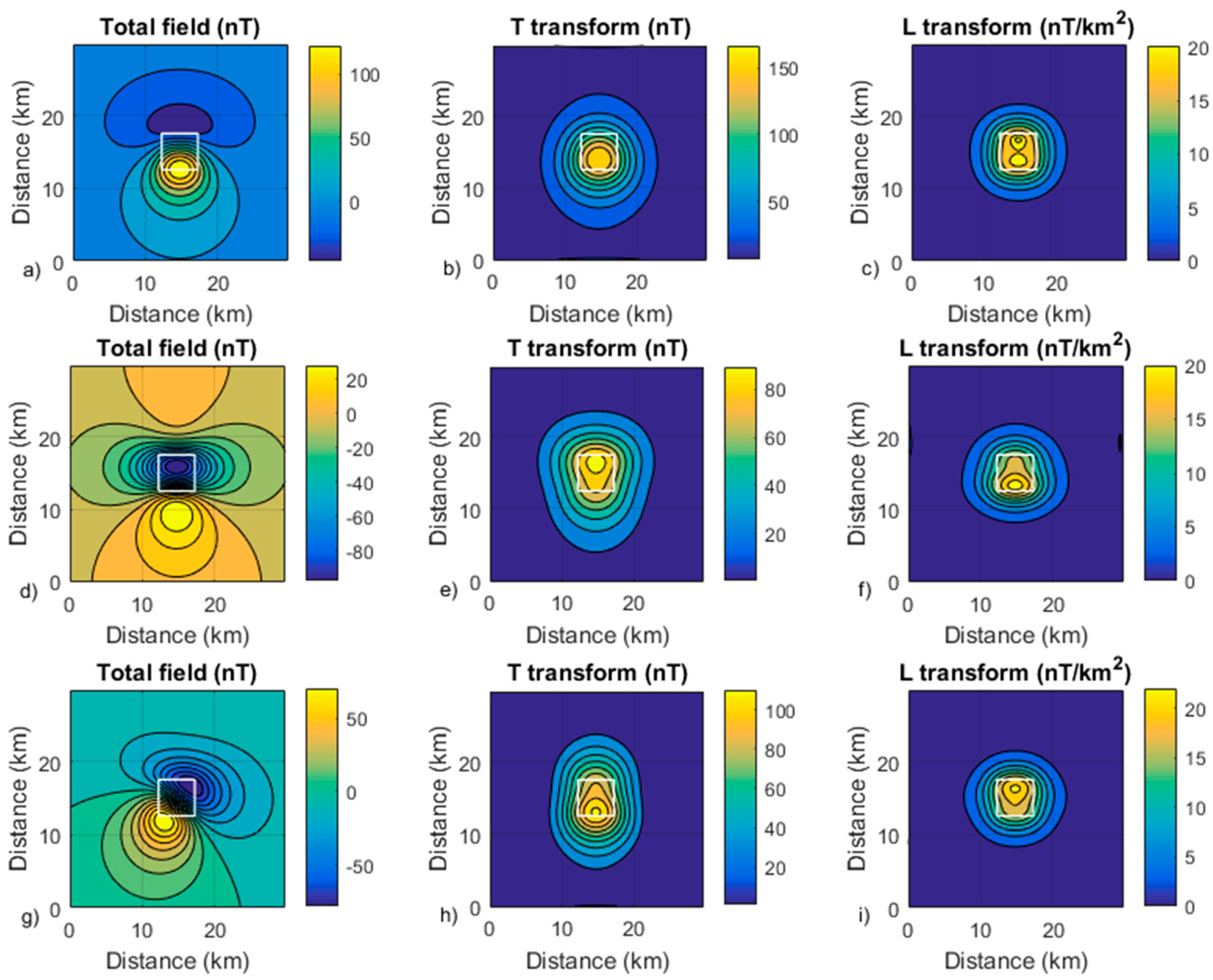
  • Similar to the reduction to the pole, the transformed field has a simple relationship with their sources, being rather independent of the magnetization direction;
  • Their computation does not require unknown quantities in input, differently from the reduction to the pole;
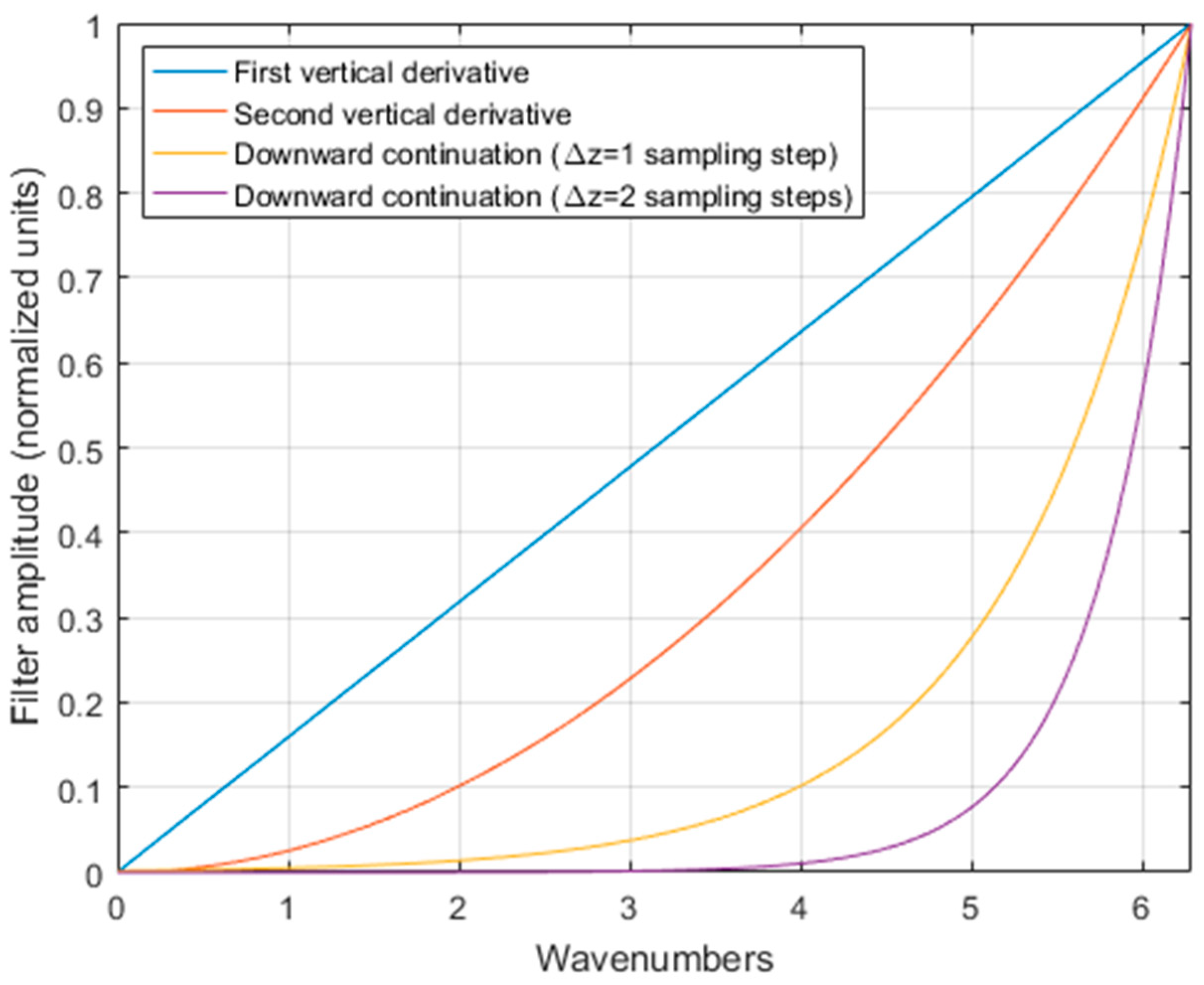
  • The transformed field shows an increased resolving power with respect to the original field, because their computation includes a differentiation process.
These transforms are based on the computation of the modulus of the anomalous magnetic intensity, T, defined as [14]:
T = X 2 + Y 2 + Z 2
where X, Y, and Z are the three Cartesian components of the total field magnetic anomaly vector, which can be directly measured or computed from the total field data by a directional integration and differentiation process [14]. As shown in Equation (1), T is always positive. Starting from Equation (1), ref. [14] defined a set of four magnetic transforms based on differential operators, such as the gradient or the Laplacian of T, able to differently enhance the measured field. In this study, to enhance the information content of low-resolution aeromagnetic datasets, we needed strong amplification of the high-wavenumbers part of the spectrum; thus, we propose using the L-transform, based on second-order derivatives of T [14]:
L = 2 T = ( | X | 2 + | Y | 2 + | Z | 2 | T | 2 ) / X 2 + Y 2 + Z 2
Ref. [14] showed that L is always positive.
We refer readers to the original paper by Stavrev and Gerovska [14] for an in-depth analysis of the properties of these transforms. In Figure 2, we show, in practice, what the effects of the transformation of the total field into T or L fields are. To this aim, we computed the total field of a square-based prismatic source with 5 km long sides, at a depth to the top of 2.5 km and a thickness of 12.5 km (we used the formulas presented in [15]). In (a), the total source magnetization is parallel to a geomagnetic field with a declination of 0° and inclination of 50° (mid-latitude case). The total field (Figure 2a) shows a dipolar form, with a complex relationship between the anomaly and the source positions. Notably, the magnetic anomaly extends over practically all the sampled area. The anomalous magnetic intensity T (Figure 2b; Equation (1)) instead presents a single maximum, almost perfectly positioned above the source. The area interested by the T anomaly is smaller than that of the corresponding total field anomaly (Figure 2a). This suggests that in real applications, the T field should be less affected by interference from the magnetic effects of nearby sources than the original total field. The Laplacian of T (i.e., the L-transform, Equation (2)) implies a second-order differentiation process, with an amplification of the high-wavenumber part of the spectrum. The L field has a maximum which is very well centered above the source. Furthermore, differently from the total field or the T transform (Figure 2a,b), the contours of L-transform (Figure 2c) do not have a round shape, their shape providing some information about the true source shape. These features, as well as the reduced horizontal extension of the L anomaly, demonstrate the effect of the increase in resolution compared with the original total field anomaly. These general features of the T- and L-transformed anomalies can also be seen in the low-latitude case (Figure 2d–f) and when there is a strong component of remanent magnetization (Figure 2g–i), confirming that these transforms are very stable with respect to the source magnetization direction [14].
This simple analysis showed the benefits that these transformations can bring to the interpretation of magnetic anomaly data. Thus, our workflow for enhancing high-altitude regional aeromagnetic data in the Tyrrhenian Sea area is composed of two phases:
  • Downward continuation of original magnetic anomalies to the sea-level altitude; this process was performed using the stabilized approach proposed by [13];
  • Computation of the L-transform of the downward continued data to obtain a high-resolution field, easily relatable with the position of their sources.
It is clear that the increase in resolution obtainable by the above workflow when applied to aeromagnetic datasets is limited by the sampling theorem [16]. It defines the minimum wavenumber as the double of the grid sampling step. The grid sampling step is, in turn, related to the actual distance among the measurement lines flown during the aeromagnetic survey.
In the subsequent sections, we compare the reprocessed aeromagnetic anomalies according to our workflow with high-resolution marine magnetic data in three selected areas in the Tyrrhenian Sea. Through this comparison, we will show that the proposed processing workflow of aeromagnetic data may lead to interesting interpretative results. In areas where higher-resolution data are lacking, the reprocessed data may be as decisive as to suggest changes to previous interpretations of aeromagnetic data or, at least, very useful for deciding if higher resolution surveys in selected areas would be needed or not.

3. Geological Settings

3.1. Tyrrhenian Sea

Tyrrhenian Sea (Italy) is a Miocene–Pleistocene oceanic back-arc basin associated with the northwest subduction of the Ionian lithosphere below the Calabrian Arc [17,18]. Extensional tectonic processes related to the slab rollback started about 11 Ma ago in the prevailing east–west direction, inducing the formation of the Vavilov sub-basin (between ca. 10 Ma and 2 Ma BP) and Vavilov Seamount (4.3–2.6 My [19,20]). The subsequent slab retreat led to the opening of the Marsili Sub-Basin (ca. 2 Ma to 0.2 Ma [21,22]) and the emplacement of Marsili Seamount. This large-scale extension produced the onset of volcanism throughout the Tyrrhenian Sea and the surrounding coasts [23,24,25]. High values of heat flow (>150 mW m−2 [26]), thin crust (7 km on average), and the presence of basaltic crust in the Marsili Basin [19,21] demonstrated the young formation age of oceanic crust in the Tyrrhenian Sea. OIB–MORB type characterizes the Vavilov Basin, whereas basalts from Marsili Basin show a more complex history, with additional calc-alkaline components [27,28].

3.2. Marsili Seamount

Marsili Seamount (MS) is an elongated volcanic structure located in the center of the deepest Tyrrhenian plain at 3500 m bsl. MS elongates ca. 70 km in the N 10° E direction, is 30 km wide, and its summit reaches ca. 500 m bsl. Due to its position and shape, MS was interpreted as the spreading center of the Marsili back-arc basin [28]. Residual magnetic anomalies allowed calculating an average spreading rate of 2.8–3.1 cm/year for this back-arc basin [29]. However, further studies, mainly based on magnetic anomalies [30] and morphology [31], suggest that MS cannot be interpreted as a classical spreading ridge. MS morphology shows a wide range of volcanic shapes, with prevailing dikes and aligned cones in the central part (at depths from −1150 to −600 m bsl), whereas the presence of flat-topped edifices occurs in the northernmost sector [31]. According to [32], these morphologic differences between volcanic structures are potentially due to different eruption rates, with smooth and flat-topped edifices emplaced by slower effusion rates and lower magma pressures.

3.3. Ischia Island

Ischia Island belongs to the Phlegrean Volcanic District, characterized by extension and volcanism during the Pliocene–Quaternary [33]. Ischia volcanic activity started ca. 135 ka [34] and consisted of a major ignimbritic eruption (Green Tuff, occurring at 55 ka [35]) and a large number of small-to-medium events, also inferred to occur at sea [36]. Ischia Island represents the uppermost part of a larger volcanic complex [2] characterized by high seismicity [37], hydrothermal activity [38,39], and vertical ground motion, whereas triggered the uplift of Mt. Epomeo, the highest relief on the island, over the last 33 ky [34]. Primary northwest–southeast, northeast–southwest and, subordinately, north–south and east–west fracture systems control volcanic activity and the resurgence of Mt. Epomeo [40,41].

3.4. Gaeta Gulf

The Gaeta Gulf is located in the uppermost sector of the Campanian–Latium offshore, characterized by lithospheric thinning and volcanism during the Pliocene–Quaternary [42]. The fault pattern of the Campania margin is marked by structures trending east–west, northeast–southwest, and northwest–southeast [43,44,45,46,47]. Tectonic subsidence has allowed the emplacement of a 4000 m thick Pliocene–Quaternary basin [44,45] and magma ascents mostly align along a regional lineament trending east–west along the 41° N parallel [48]. This lineament is characterized by the alignment of several magnetic anomalies extending for about 150 km, ending on land in correspondence to a buried lava intrusion north of Phlegrean Fields [49]. The 41° N parallel lineament, interpreted as a strike-slip [50], a transform [51], or as a transfer fault [42], is not associated with any relevant seafloor morphology. In the Gaeta Gulf, polygenic volcanic activity led to the onset of ancient (4.2 to 1.0 Ma) rhyolitic volcanic edifices in Ponza, Zannone, and Palmarola Islands [52], whereas younger (0.8 to 0.13 Ma) and less acidic products can be found at Ventotene Island.

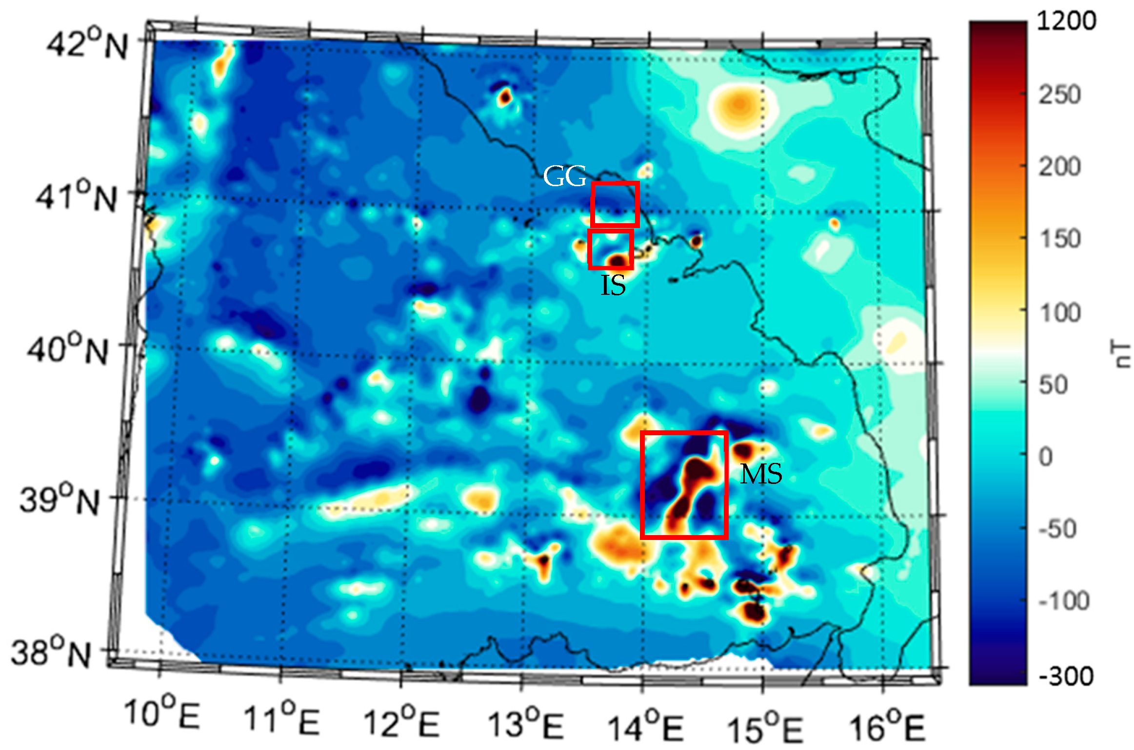
4. Comparison of Enhanced Aeromagnetic Data with Shipborne Magnetic Data in Three Selected Areas in the Tyrrhenian Sea

In this section, we first describe the aeromagnetic data of the Tyrrhenian Sea to be enhanced by the workflow proposed in Section 2. Then, we focus on the comparison of the enhanced aeromagnetic data with shipborne higher resolution data available in three selected areas in the Tyrrhenian Sea (namely, the western offshore of Ischia Island, the Gaeta Gulf, and the Marsili Seamount).

4.1. Aeromagnetic Data

In the frame of programs aimed at the hydrocarbon research, during the decade 1970–1980, the former Italian oil company (AGIP) carried out an aeromagnetic survey covering the entire Italian territory, using scalar, Cesium-vapor magnetometers. The constant flight altitude, as well as the spacing of survey and control lines, varied in the Italian region according to the terrain elevation [53]. In the Tyrrhenian Sea area, the constant flight altitude was 1463 m above sea level, with 5 km spaced southwest–northeast survey lines and 7.5 km spaced, perpendicular tie lines. Near to coastal areas, the survey line spacing was 2.5 km, and even smaller locally [54]. The aeromagnetic maps at 1:500,000 scale covering the Tyrrhenian Sea area were digitized and a 2 km spaced grid was obtained. The resulting map, after the subtraction of a constant value of 3077 nT, is shown in Figure 3.
The great complexity of the Tyrrhenian aeromagnetic field is exhibited by the presence of many patterns of anomalies related to the presence of geological structures whose nature and origin are, in some cases, still uncertain [55]. Most of the magnetic anomalies in the area can be related to volcanic rocks or shallow intrusions in the young Tyrrhenian oceanized crust. High-amplitude anomalies are present in the southeast area, in correspondence to the Aeolian Islands and the Marsili and Palinuro Seamounts. Aligned anomalies, trending east-northeast–west-southwest, are clearly visible in the southwestern part of the basin, as well as reversed anomaly generated by the magnetized structures of the Vavilov Seamount, at the center of the map.

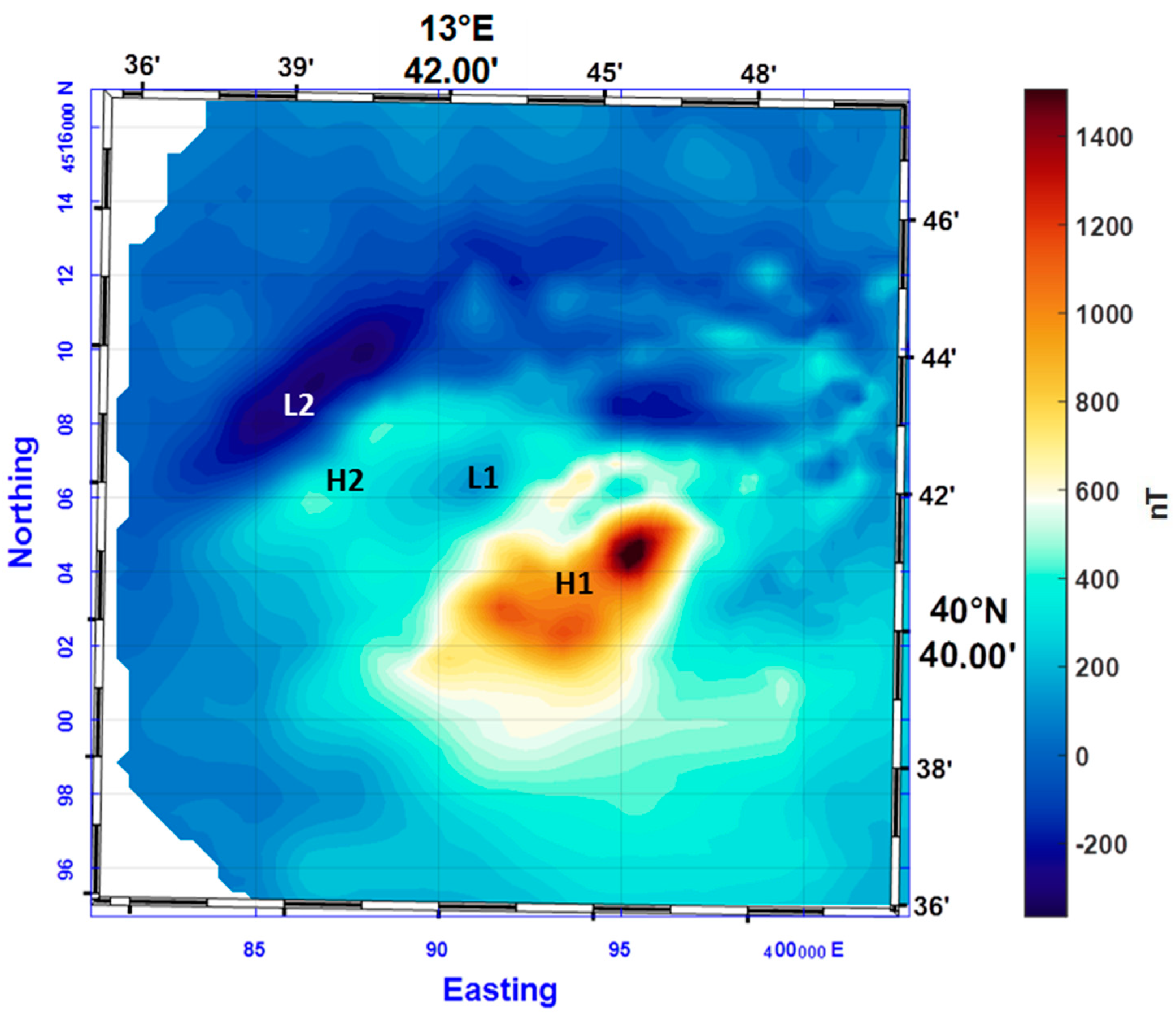
4.2. Magnetic Data in the Ischia Area

In the offshore area west of the Ischia Island (located in box IS in Figure 3), the shipborne magnetic data are based on a survey carried out in 2000 by employing a proton magnetometer towed at 250 m from a ship and at 20–25 m depth. The survey lines were north–south oriented and their spacing (1.5 or 0.75 km) enabled computation of a magnetic anomaly map with a 375 × 375 m2 cell grid size. The high resolution of the data sampling highlighted the presence of magnetic anomalies (Figure 4) spatially correlated with two main east–west and northeast–southwest volcanic ridges and with the presence of magma intrusions often emplaced along regional northeast–southwest tectonic features [2].
An intense dipolar anomaly (more than 1200 nT at sea level) is located on the southern flank of a bathymetric northeast–southwest ridge (H1 and L1 in Figure 4). Another southwest–northeast elongated anomaly is present in the westernmost area (H2 and L2 in Figure 4), having an anomalously intense and extended low area, exhibiting the presence of an intrusion with a probable large remanent component in the total magnetization. Moreover, this anomaly does not correlate with any seafloor feature, that in this area, is relatively flat. Northeastward, several small anomalies form a rather complex pattern, probably due to the coalescence of highs and lows of anomalies caused by small and shallow body sources very close to each other.
The aeromagnetic anomalies of the western offshore of the Ischia Island show only a single large dipolar anomaly (H1–L1 in Figure 5) extended over a 30 × 30 km2 surface and with a peak-to-throw axis in a northwest–southeast direction, a direction very different from the current declination of the main geomagnetic field in this area. The knowledge of the higher-resolution magnetic field at sea level [2] implies that the aeromagnetic single anomaly is actually the result of coalescence effects at the flight altitude (1463 m above sea level); thus, any interpretation of the aeromagnetic anomaly as generated from a single source [56] is misleading.
Continuing the aeromagnetic field downward to sea level enriched the magnetic map with many features, more complex than a single main dipolar anomaly (Figure 6). As an example, a weak magnetic low (L1 in Figure 6) appears in correspondence of the low related to the southeastern high visible in the shipborne data map (L1 in Figure 4). However, the enhancement of high wavenumbers given by the downward continuation to sea level is still not sufficient to resolve the main dipolar anomaly into more interfering components and clearly identifying the northwest anomaly visible in the shipborne dataset (H2–L2 in Figure 4).
A much greater resolution improvement was achieved by computing the L-transform of the airborne data continued to sea level. The L-transform presents two intense highs with elongated shapes aligned in the southwest–northeast direction (Figure 7). These highs are highly spatially correlated with the main magnetic anomalies in the shipborne survey. In fact, the southern L-transform high (A in Figure 7) corresponds to a southwest–northeast bathymetric ridge, whereas the northern L-transform high (B in Figure 7) corresponds to the expected source position of the western southwest–northeast elongated shipborne anomaly (H2–L2 in Figure 4). In fact, as explained in Section 2, the L-transform of a dipolar anomaly presents a single high in correspondence to the magnetic source, being rather independent of the source magnetization direction.
Thus, we see that, in this case, the processing workflow of the aeromagnetic anomalies revealed very important insights into the structure of the magnetized shallow crust, showing the strong limitations of a simple qualitative interpretation of the original aeromagnetic data.

4.3. Magnetic Data in the Gaeta Gulf Area

The shipborne magnetic data in the Gaeta Gulf (located in box GG in Figure 3) were collected during two oceanographic cruises in 1992 and 1993 along survey lines oriented northwest–southeast and northeast–southwest, by employing a proton magnetometer towed 250 m from the ship and at 10–40 m depth. After standard processing, the data were interpolated on a 750 × 750 m2 cell grid size.
The shipborne magnetic anomaly map shows a sharp anomaly with reversed polarity (H1–L1 in Figure 8). This anomaly was interpreted as a high susceptibility east–west elongated volcanic edifice, with a high remanent magnetization component along a direction opposite from that of the present inducing field [57]. It is interesting to notice that this reversed anomaly is hard to identify in the aeromagnetic data, because it lies in an area where many magnetic lows develop (L2 and L3 in Figure 8), related to normally magnetized buried sources emplaced further south.
In fact, the case of the anomaly of the Gaeta Gulf well shows the loss of information and the ambiguity of interpretation due to the high measurement altitude of an aeromagnetic survey. The map of the aeromagnetic field (Figure 9) shows only a single magnetic low (L1 in Figure 9) in the investigated area, whereas there is no evidence of the small and weak magnetic high visible northward in the shipborne data map (H1 in Figure 8). In this case, the low resolution and the great distance from the causative source affect the correct representation of the shape of the anomaly, concealing an essential attribute such as its dipolar character. This can compromise any attempt of analysis, thus causing misleading interpretations.
The downward continuation of the airborne data to sea level highlights the dipolar character of the main anomaly, by the presence of a small magnetic high north of the main low (L1–H1 in Figure 10). The magnetic low in the downward continued magnetic anomaly map has approximately the same shape and position of the main anomaly visible in the map from shipborne data. The only difference consists of the geographic position of the relative high, shifted slightly eastward (~2000 m) with respect to that shown in the shipborne magnetic map. This mislocation is probably generated by the large spacing among the airborne survey lines (5 km). The map of the L-transform of the airborne data continued to sea level returns a well-evidenced maximum located at the position of the main anomaly source (Figure 11). The magnetic high in the L-transform map appears slightly elongated westward just as the shipborne magnetic anomaly (L1 in Figure 8).
This case showed the benefits of the increase in resolution provided by our workflow that singled out the magnetic anomaly generated by a reverse-magnetized volcanic source. Moreover, because the L-transform is relatively independent from the unknown source magnetization, it was possible to easily and unambiguously locate the anomalous source on the map.

4.4. Magnetic Data in the Marsili Seamount Area

A high-resolution shipborne magnetometric survey was carried out in the area of the Marsili Seamount (located in the box MS in Figure 3) during 2006 [58]. Data were collected with a Cesium magnetometer along east-southeast–west-northwest track lines, with the spacing gradually decreasing from 15 km to 3 km toward the central area of the seamount. The grid of the total magnetic field over the MS area has a cell size of 500 × 500 m2 [29]. The total field anomalies (Figure 12) show a series of highs along the seamount crest and deep lows in the northwest area. Other magnetic lows are present to the north and to southeast of the seamount. The geodynamical context, in a young back-arc basin, the elongated shape of the seamount and its overall dimensions lead several authors to interpret the magnetic anomalies in the MS basin as an expression of the oceanized floor expansion, with the presence of bands of crust magnetized with alternating polarity [20]. The analysis of aeromagnetic data and of its anomalous magnetic intensity [30] demonstrated the diffuse presence of reverse-magnetized rocks in the MS basin, although they could not confirm the presence of a well-organized striped pattern of magnetic anomalies. However, the analysis of the higher-resolution shipborne magnetic dataset of Figure 12 highlighted the presence of subtle, low-amplitude, elongated highs developing symmetrically to the MS axis, in its northern part [29]. These symmetric magnetic highs were interpreted as generated by magnetized structures at the base of the volcanic edifice dating back to Jaramillo subchron (about 1 million years ago), marking the transition from lateral spreading to a phase with prevailing vertical growth of the seamount [29].
The map of aeromagnetic anomalies shows two main highs (H1 and H2 in Figure 13) at the northern and southern ends of the MS, whereas three lows are visible along its western slope (L1, L2, and L3 in Figure 13) and only one low is located on its eastern slope (L4 in Figure 13).
The shipborne magnetic map (Figure 12) shows a number of small details not visible in the aeromagnetic map. It consists of a complex pattern of several highs and lows that cannot easily be coupled in dipolar anomalies because of a coalescence of effects and the presence of reverse magnetization. Most of them seem to be distributed perpendicular to the main axis of the MS and the alternance of highs and lows (in Figure 12, from the seamount axis towards the northwest: H1, L4, H8, L5, and H9; from the seamount axis towards the southeast: H6, L2, H7) was interpreted as the result of the spreading evolution of the Marsili Basin [29]. Along the central axis there is a presence of other small anomalies as H2 and H3 highs (Figure 12) or L3 and L6 magnetic lows flanking the seamount from both sides (Figure 12).
The downward continuation of the aeromagnetic anomalies to sea level (Figure 14) produces a noticeable increase in information. The aeromagnetic field presents many similarities to the pattern of anomalies recognized in the shipborne data (e.g., L1, H4, H5 and H10). In particular, the two small peaks placed in the central part of the Seamount in shipborne magnetic anomalies are also detectable in the airborne data continued to sea level (H3 an H2 in Figure 14). The same applies for most of the low-amplitude highs and lows already shown in the shipborne data map along the western and the eastern side of the seamount (in Figure 14, from the seamount axis towards the northwest: H1, L4–L5 and H8–H9; from the seamount axis towards the southeast: H6 and L2). As in the shipborne data, are also visible magnetic lows L3 and L6 flanking the seamount from both sides (Figure 14). However, in the magnetic field continued downward to sea level, it is still not possible to see some features visible in the map from shipborne survey, such as the central low (L1 in Figure 12) interpreted as due to a crustal volume demagnetized by hydrothermal alteration [29], or the high H6 in Figure 12, only barely detectable in the airborne data continued downward.
The analysis of the L-transform of the total field downward continued to sea level allowed establishing a spatial correlation between each anomaly and the corresponding crustal source, regardless of whether the magnetization is normal or reversed. In Figure 15, the anomalies A, B, C, D and G appears easily relatable to the magnetized structure of the MS. More interestingly, the map of the L-transform (Figure 15) shows several roughly parallel and northeast–southwest elongated highs, having a short length (about 20 km, at most). On the northwest side, such elongated features are the anomalies L and M and I (Figure 15). On the southeast slope of the seamount, other elongated features of the L-transform map can be observed, such as the subtle E–H anomaly and the F anomaly, located on the external margin of the eastern slope (Figure 15). In some cases, the above magnetic features seem to be correlated with the sea-floor morphology: anomaly I apparently corresponds to a small, thin ridge placed just at the base of the western Marsili slope, whereas linear anomaly F seems to be related to a bathymetric step of the sea bottom at the base of the eastern slope.
Although sometimes having a slightly different location, these features of the enhanced aeromagnetic field are clearly relatable to the subtle total field symmetric anomalies interpreted as demonstrating the spreading evolution of the Marsili Basin [29]. Detailed modelling of the aeromagnetic L anomalies would be not an easy task. However, in the absence of a marine dataset, these results would indicate the presence of magnetic features of interest that may be the target for further detailed surveys.

5. Discussion and Conclusions

This analysis has not aimed to propose new methodological tools for the processing of magnetic data. Moreover, we have demonstrated how the combination of two well-known magnetic field transformations can be very helpful to increase the information content of high-altitude, low-resolution aeromagnetic data. Sometimes, the information increase is such that it leads to anomalies completely different from the original ones. In this paper, we have shown that the transformed aeromagnetic data compare very well with high-resolution shipborne magnetic datasets, confirming the consistency and the utility of the proposed workflow.
From the examples illustrated here, it is clear that in the case of the Italian aeromagnetic dataset, the simple processing proposed can greatly enrich the information content of the magnetic maps.
In the Western undersea section of the Ischia volcanic complex and in the Gaeta Gulf cases, the contribution given by our processing workflow to the correct interpretation of aeromagnetic data was evident. In both cases, the interpretation of the aeromagnetic map at the original flight altitude would have been misleading because of the interference and coalescence effects. Moreover, in both cases, the shape of some anomalies demonstrates the presence of a strong component of remanent magnetization, complicating the magnetic pattern and any modelling attempt.
As we have shown, in the Ischia case, the L-transformed data continued downward resolves a single, abnormally shaped, aeromagnetic anomaly (the peak-to-through axis deviates from the direction of the local magnetic meridian) into two distinct anomalies that correlate very well to magnetic features visible in the shipborne magnetic anomaly map. These two anomalies are, in turn, relatable to two main magmatic bodies: the first corresponds to an east-northeast–west-southwest volcanic ridge with a clear morphological expression; the second, almost parallel to the previous ridge, does not show a clear morphological signature and suggests a deeper intrusion controlled by the local southwest–northeast tectonic trend [2].
In the Gaeta Gulf case, a reverse-magnetized source producing an anomaly hidden in a vast area with magnetic lows (related to the presence, further south, of normally magnetized sources along the 41° parallel lineament) was clearly evidenced and correctly positioned, in spite of the unknown magnetization of the sources, by the L-transform of the data continued downward.
In the Marsili area, the L-transform of the aeromagnetic data continued downward evidenced the presence of several linear anomalies otherwise not visible in the original dataset. These linear features could be related to magnetization inhomogeneity, perhaps due to the cooling of magmatic masses under the influence of the Earth’s magnetic field with different polarities. Some of the L-transform elongated anomalies may also be related to local seafloor morphologies. These linear anomalies in the L-transform map cannot exactly be spatially correlated to the subtle linear anomalies seen in the shipborne total field. However, we believe that, if no shipborne data were available, their presence would be suggestive of the importance of more detailed investigations in the area. Thus, the processing of aeromagnetic data can help to identify areas of special interest for detailed local magnetic surveys.
The proposed workflow proved its efficiency in improving the resolution and readability of aeromagnetic maps in the Tyrrhenian area. The downward continuation and the differentiation implied in the L-transform enhance the high-wavenumber part of the spectrum, increasing the possibility of identifying details in the transformed magnetic maps and effectively separating the contributions due to nearby sources. Moreover, the L-transform directly provides anomalies located at the horizontal position of their sources, as it is relatively independent from the unknown total magnetization direction of the magnetic sources. In long-lasting, back-arc, volcanic settings such as the Tyrrhenian Sea, this is very useful, as reduction to the pole is not easily applicable because the magnetization direction is generally unknown and due to the coexistence of sources magnetized in different directions in the same area.
The transformed anomalies can be directly used for qualitative interpretation of large-scale airborne/satellite datasets analyzed in regional studies of magnetic anomalies [59,60]. In some cases, they may be used to identify areas of special interest worth magnetic exploration by a high-resolution shipborne survey. Therefore, before planning a marine magnetometric survey, we suggest studying the transformed aeromagnetic field according to our proposed workflow, which may allow for accurate selection of the areas of greatest scientific interest.
It is clear that the proposed enhancement of aeromagnetic data tends to increase the power of the high-wavenumber part of the spectrum, so that any noise present in the original data may be strongly enhanced if no special treatment is adopted in the downward continuation as well as in the differentiations needed to compute the L-transform. We used a stabilized algorithm for both the downward continuation [13] and for the vertical differentiation (the ISVD scheme [61]), while the horizontal derivatives were stably computed in the space domain through a simple finite difference algorithm.
As a final remark, of course, even shipborne magnetic dataset may benefit from such a processing, further decreasing the anomaly interference and producing a high-resolution alternative to commonly used reduced to pole maps.

Author Contributions

Conceptualization, G.F., F.C., S.P. and G.d.A.; methodology, G.F.; software, G.F.; validation, F.C.; formal analysis, G.F. and F.C.; investigation, G.F. and F.C.; data curation, G.F., F.C., S.P. and G.d.A.; writing—original draft preparation, G.F. and F.C.; writing—review and editing, G.F., F.C., S.P. and G.d.A.; visualization, F.C. All authors have read and agreed to the published version of the manuscript.

Funding

This research received no external funding.

Data Availability Statement

The data presented in this study are not publicly available due to 3rd party data restrictions.

Acknowledgments

The authors warmly thank the Academic Editor and three anonymous reviewers for their comments and criticism that helped to improve the original submission.

Conflicts of Interest

The authors declare no conflict of interest.

References

  1. Salem, A.; Mohammed, Y.A. Mapping Basement Structures in the Northwestern Offshore of Abu Dhabi from High-Resolution Aeromagnetic Data. Geophys. Prospect. 2016, 64, 726–740. [Google Scholar] [CrossRef]
  2. Bruno, P.P.G.; de Alteriis, G.; Florio, G. The Western Undersea Section of the Ischia Volcanic Complex (Italy, Tyrrhenian Sea) Inferred by Marine Geophysical Data. Geophys. Res. Lett. 2002, 29, 57-1–57-4. [Google Scholar] [CrossRef] [Green Version]
  3. Grauch, V.J.S.; Hudson, M.R.; Minor, S.A. Aeromagnetic expression of faults that offset basin fill, Albuquerque basin, New Mexico. Geophysics 2001, 66, 707–720. [Google Scholar] [CrossRef]
  4. Li, Y.; Sun, J.; Li, S.L.; Leão-Santos, M. A paradigm shift in magnetic data interpretation: Increased value through magnetization inversions. Lead. Edge 2021, 40, 89–98. [Google Scholar] [CrossRef]
  5. Fedi, M.; Florio, G.; Rapolla, A. 2.5D Modelling of Somma–Vesuvius Structure by Aeromagnetic Data. J. Volcanol. Geotherm. Res. 1998, 82, 239–247. [Google Scholar] [CrossRef]
  6. Bouligand, C.; Glen, J.M.G.; Blakely, R.J. Distribution of Buried Hydrothermal Alteration Deduced from High-Resolution Magnetic Surveys in Yellowstone National Park. J. Geophys. Res. Solid Earth 2014, 119, 2595–2630. [Google Scholar] [CrossRef]
  7. Pilkington, M.; Tschirhart, V. Practical Considerations in the Use of Edge Detectors for Geologic Mapping Using Magnetic Data. Geophysics 2017, 82, J1–J8. [Google Scholar] [CrossRef]
  8. Okubo, Y.; Graf, R.J.; Hansen, R.O.; Ogawa, K.; Tsu, H. Curie Point Depths of the Island of Kyushu and Surrounding Areas, Japan. Geophysics 1985, 50, 481–494. [Google Scholar] [CrossRef]
  9. Accomando, F.; Vitale, A.; Bonfante, A.; Buonanno, M.; Florio, G. Performance of Two Different Flight Configurations for Drone-Borne Magnetic Data. Sensors 2021, 21, 5736. [Google Scholar] [CrossRef]
  10. Galley, C.G.; Jamieson, J.W.; Lelièvre, P.G.; Farquharson, C.G.; Parianos, J.M. Magnetic Imaging of Subseafloor Hydrothermal Fluid Circulation Pathways. Sci. Adv. 2020, 6, eabc6844. [Google Scholar] [CrossRef]
  11. Blakely, R.J. Potential Theory in Gravity and Magnetic Applications; Cambridge University Press: Cambridge, UK, 1995. [Google Scholar] [CrossRef]
  12. Evjen, H.M. The place of the vertical gradient in gravitational interpretations. Geophysics 1936, 1, 127–136. [Google Scholar] [CrossRef]
  13. Fedi, M.; Florio, G. A Stable Downward Continuation by Using the ISVD Method. Geophys. J. Int. 2002, 151, 146–156. [Google Scholar] [CrossRef] [Green Version]
  14. Stavrev, P.; Gerovska, D. Magnetic Field Transforms with Low Sensitivity to the Direction of Source Magnetization and High Centricity. Geophys. Prospect. 2000, 48, 317–340. [Google Scholar] [CrossRef]
  15. Bhattacharyya, B.K. Magnetic anomalies due to prism-shaped bodies with arbitrary polarization. Geophysics 1964, 29, 517–531. [Google Scholar] [CrossRef]
  16. Oppenheim, A.V.; Schafer, R.W.; Buck, J.R. Discrete Time Signal Processing, 2nd ed.; Prentice Hall: Hoboken, NJ, USA, 1989. [Google Scholar]
  17. Malinverno, A.; Ryan, W.B.F. Extension in the Tyrrhenian sea and shortening in the Apennines as result of Arc migration driven by sinking of the lithosphere. Tectonics 1986, 5, 227–245. [Google Scholar] [CrossRef]
  18. Cella, F.; de Lorenzo, S.; Fedi, M.; Loddo, M.; Mongelli, F.; Rapolla, A.; Zito, G. Temperature and density of the Tyrrhenian lithosphere and slab and new interpretation of gravity field in the Tyrrhenian Basin. Tectonophysics 2006, 412, 27–47. [Google Scholar] [CrossRef]
  19. Kastens, K.A.; Mascle, J.; Auroux, C.; Bonatti, E.; Broglia, C.; Channell, J.; Curzi, P.; Emeis, K.; Glacon, G.; Hasegawa, S.; et al. ODP Leg 107 in the Tyrrhenian Sea: Insights into passive margin and back-arc basin evolution. Geol. Soc. Am. Bull. 1988, 100, 1140–1156. [Google Scholar] [CrossRef]
  20. Savelli, C.; Schreider, A.A. The opening processes in the deep Tyrrhenian basin of Marsili and Vavilov, as deduced from magnetic and chronological evidence of their igneous crust. Tectonophysics 1991, 190, 119–131. [Google Scholar] [CrossRef]
  21. Kastens, K.A.; Mascle, J.; Auroux, C.; Bonatti, E.; Broglia, C.; Curzi, P.; Emeis, K.C.; Glacon, G.L.; Hasegawa, S.; Hieke, W.; et al. The geological evolution of the Tyrrhenian Sea: An introduction to the scientific results of ODP Leg 107. In Proceedings of the ODP Scientific Results; Kastens, K.A., Mascle, J., Eds.; Ocean Drilling Program: College Station, TX, USA, 1990; Volume 107, p. 26. [Google Scholar] [CrossRef]
  22. Savelli, C. Two-stage progression of volcanism (8-0 Ma) in the central Mediterranean (southern Italy). J. Geodyn. 2001, 31, 393–410. [Google Scholar] [CrossRef]
  23. Beccaluva, L.; Rossi, P.L.; Serri, G. Neogene to Recent volcanism of the Southern Tyrrhenian–Sicilian area: Implications for the geodynamic evolution of the Calabrian Arc. Earth Evol. Sci. 1982, 3, 222–238. [Google Scholar]
  24. Beccaluva, L.; Gabbianelli, G.; Lucchini, F.; Rossi, P.L.; Savelli, C. Petrology and K/Ar ages of volcanic dredged from the Eolian seamounts: Implications for geodynamic evolution of the Southern Tyhrrenian basin. Earth Planet. Sci. Lett. 1985, 74, 187–208. [Google Scholar] [CrossRef]
  25. Turco, E.; Zuppetta, A. A kinematic model for the Plio-Quaternary evolution of the Tyrrhenian–Apenninic system: Implications for rifting processes and volcanism. J. Volcanol. Geoth. Res. 1998, 82, 1–18. [Google Scholar] [CrossRef]
  26. Della Vedova, B.; Pellis, G.; Foucher, J.P.; Rhéault, J.-P. Geothermal structure of the Tyrrhenian Sea. Mar. Geol. 1984, 55, 271–289. [Google Scholar] [CrossRef]
  27. Beccaluva, L.; Bonatti, E.; Dupuy, C.; Ferrara, G.; Innocenti, F.; Lucchini, F.; Macera, P.; Petrin, R.; Rossi, P.L.; Serri, G.; et al. Geochemistry and Mineralogy of Volcanic Rocks from ODP Sites 650, 651, 655, and 654 in the Tyrrhenian Sea. In Proceedings of the ODP Scientific Results; Kastens, K.A., Mascle, J., Eds.; Ocean Drilling Program: College Station, TX, USA, 1990; Volume 107, pp. 49–74. [Google Scholar]
  28. Trua, T.; Serri, G.; Marani, M.; Renzulli, A.; Gamberi, F. Volcanological and petrological evolution of Marsili seamount (Southern Tyrrhenian Sea). J. Volcanol. Geotherm. Res. 2002, 114, 441–464. [Google Scholar] [CrossRef]
  29. Cocchi, L.; Caratori Tontini, F.; Muccini, F.; Marani, M.P.; Bortoluzzi, G.; Carmisciano, C. Chronology of the transition from a spreading ridge to an accretional seamount in the Marsili backarc basin (Tyrrhenian Sea). Terra Nova 2009, 21, 369–374. [Google Scholar] [CrossRef]
  30. Florio, G.; Fedi, M.; Cella, F. Insights on the spreading of Tyrrhenian Sea from the magnetic anomaly pattern. Terra Nova 2011, 23, 127–133. [Google Scholar] [CrossRef]
  31. Ventura, G.; Milano, G.; Passaro, S.; Sprovieri, M. The Marsili ridge (Southern Tyrrhenian Sea, Italy): An island-arc volcanic complex emplaced on a ‘relict’ back-arc basin. Earth Sci. Rev. 2013, 116, 85–94. [Google Scholar] [CrossRef]
  32. Head, I.I.I.J.W.; Wilson, L.; Smith, D.K. Mid-ocean ridge eruptive vent morphology and substructure: Evidence for dike widths, eruption rates, and evolution of eruptions and axial volcanic ridges. J. Geophys. Res. 1996, 101, 28265–28280. [Google Scholar] [CrossRef]
  33. D’Antonio, M.; Tonarini, S.; Arienzo, I.; Civetta, L.; Di Renzo, V. Components and processes in the magma genesis of the Phlegrean volcanic district, Southern Italy. Spec. Pap. Geol. Soc. Am. 2007, 418, 203–220. [Google Scholar]
  34. Gillot, P.Y.; Chiesa, S.; Pasquaré, G.; Vezzoli, L. 33.000 yr K/Ar dating of the volcano-tectonic horst of the isle of Ischia, Gulf of Naples. Nature 1982, 229, 242–245. [Google Scholar] [CrossRef]
  35. Vezzoli, L. Island of Ischia. Quaderni de “La ricerca scientifica” progetto finalizzato “geodinamica”. Monogr. Final. 1998, 10, 134. [Google Scholar]
  36. Passaro, S.; de Alteriis, G.; Sacchi, M. Bathymetry of Ischia Island and its offshore (Italy), scale 1:50.000. J. Maps 2016, 12, 152–159. [Google Scholar] [CrossRef]
  37. Cusano, P.; Petrosino, S.; De Lauro, E.; Falanga, M. The whisper of the hydrothermal seismic noise at Ischia Island. J. Volcanol. Geotherm. Res. 2020, 389, 106693. [Google Scholar] [CrossRef]
  38. Chiodini, G.; Avino, R.; Brombach, T.; Caliro, S.; Cardellini, C.; De Vita, S.; Frondini, F.; Granirei, D.; Marotta, E.; Ventura, G. Fumarolic and diffuse soil degassing west of Mount Epomeo, Ischia, Italy. J. Volcanol. Geotherm. Res. 2004, 133, 291–309. [Google Scholar] [CrossRef]
  39. Paoletti, V.; Di Maio, R.; Cella, F.; Florio, G.; Motschka, K.; Roberti, N.; Secomandi, M.; Supper, R.; Fedi, M.; Rapolla, A. The Ischia volcanic island (Southern Italy): Inferences from potential field data interpretation. J. Volcanol. Geotherm. Res. 2009, 179, 69–86. [Google Scholar] [CrossRef]
  40. Acocella, V.; Funiciello, R. The interaction between regional and local tectonics during resurgent doming: The case of the island of Ischia, Italy. J. Volcanol. Geotherm. Res. 1999, 88, 109–123. [Google Scholar] [CrossRef]
  41. Molin, P.; Acocella, V.; Funiciello, R. Structural, seismic and hydrothermal features at the border of an active intermittent resurgent block: Ischia Island (Italy). J. Volcanol. Geotherm. Res. 2003, 121, 65–81. [Google Scholar] [CrossRef]
  42. Trincardi, F.; Zitellini, N. The rifting of the Tyrrhenian Basin. Geo-Mar. Lett. 1987, 7, 1–6. [Google Scholar] [CrossRef]
  43. Zitellini, N.; Marani, M.; Borsetti, M. Post-orogenic tectonic evolution of Palmarola and Ventotene Basins (Pontine Archipelago). Mem. Soc. Geol. It. 1984, 27, 121–131. [Google Scholar]
  44. Bruno, P.P.G.; Di Fiore, V.; Ventura, G. Seismic study of the ‘41st parallel’ Fault System offshore the Campanian-Latial continental margin, Italy. Tectonophysics 2000, 324, 37–55. [Google Scholar] [CrossRef]
  45. Milia, A.; Torrente, M.M. Space-time evolution of an active volcanic field in an extentional region: The example of the Campania margin (eastern Tyrrhenian Sea). In Vesuvius, Campi Flegrei, and Campanian Volcanism; De Vivo, B., Belkin, H.E., Rolandi, G., Eds.; Elsevier (Rotterdam): Rotterdam, The Netherlands, 2020; Volume 12, pp. 297–321. [Google Scholar]
  46. Ortolani, F.; Aprile, F. Nuovi dati sulla struttura profonda della Piana Campana ad est del fiume Volturno. Boll. Soc. Geol. It. 1978, 97, 591–608. [Google Scholar]
  47. Mariani, M.; Prato, R. I bacini Neogenici costieri del margine tirrenico: Approccio sismico stratigrafico. Mem. Soc. Geol. Ital. 1988, 41, 519–531. [Google Scholar]
  48. Bartole, R.; Savelli, D.; Tramontana, M.; Wezel, F.C. Structural and sedimentary features in the Tyrrhenian margin off Campania, Southern Italy. Mar. Geol. 1984, 55, 163–180. [Google Scholar] [CrossRef]
  49. Barbieri, M.; Di Girolamo, P.; Locardi, E.; Lombardi, G.; Stanzione, D. Petrology of the Calc-Alkaline Volcanics of the Parete 2 Well (Campania, Italy). Period. Mineral. 1979, 48, 53–74. [Google Scholar]
  50. Wezel, F.C. Structural features and basin tectonics of the Tyrrhenian Sea. In Geological Evolution of the Mediterranean Basin; Stanley, D.J., Wezel, F.C., Eds.; Wiley: New York, NY, USA, 1985; pp. 153–194. [Google Scholar]
  51. Selli, R. Thoughts on the geology of the Mediterranean Region. In Sedimentary Basins of Mediterranean Margins; Wezel, F.C., Ed.; Tecnoprint Ed.: Bologna, Italy, 1981; pp. 489–501. [Google Scholar]
  52. De Rita, D.; Funiciello, R.; Pantosti, D.; Salvini, F.; Sposato, A.; Velonà, M. Geological and structural characteristics of the Pontine islands (Italy) and implications with the evolution of the Tyrrhenian Margin. Mem. Soc. Geol. Ital. 1986, 36, 55–65. [Google Scholar]
  53. Cassano, E.; Fichera, R.; Arisi Rota, F. Rilievo Aeromagnetico D’italia: Alcuni Risultati Interpretativi. In Atti del v Convegno Annuale del Gruppo Nazionale di Geofisica della Terra Solida; CNR: Roma, Italy, 1986; Volume 2, pp. 939–962. [Google Scholar]
  54. Caratori Tontini, F.; Stefanelli, P.; Giori, I.; Faggioni, O.; Carmisciano, C. The Revised Aeromagnetic Anomaly Map of Italy. Ann. Geophys. 2004, 47, 1547–1555. [Google Scholar] [CrossRef]
  55. Cella, F.; Fedi, F.; Florio, G.; Rapolla, A. Boundaries of magnetic anomaly sources in the Tyrrhenian Region. Ann. Geofis. 1998, 41, 433–447. [Google Scholar] [CrossRef]
  56. Fedi, M.; Rapolla, A. Aeromagnetic anomaly shape analysis in the Southern Italian Region for the evaluation of crustal block rotations. J. Geodyn. 1990, 12, 149–161. [Google Scholar] [CrossRef]
  57. de Alteriis, G.; Fedi, M.; Passaro, S.; Siniscalchi, A. Magneto-seismic interpretation of subsurface volcanism in the Gaeta Gulf (Italy, Tyrrhenian Sea). Ann. Geophys. 2006, 49, 930–943. [Google Scholar] [CrossRef]
  58. Paltrinieri, D.; Viezzoli, C.; Signanini, P.; Di Sabatino, B.; D’Anna, G.; Calcara, M.; Bortoluzzi, G.; Cocchi, L.; Caratori Tontini, F. Report on the Morphobathymetric, Magnetometric, Gravimetric, CTD, Water and Bottom Sampling Investigations during Cruise MRS06 Aboard R⁄v Universitatis; ISMAR-CNR Interim Report; ISMAR-CNR: Bologna, Italy, 2006. [Google Scholar]
  59. Milano, M.; Fedi, M.; Fairhead, J.D. The deep crust beneath the Trans-European Suture Zone from a multiscale magnetic model: Multiscale Magnetic Model of the Tesz. J. Geophys. Res. Solid Earth 2016, 121, 6276–6292. [Google Scholar] [CrossRef] [Green Version]
  60. Milano, M.; Fedi, M.; Fairhead, J.D. Joint analysis of the magnetic field and total gradient intensity in central Europe. Solid Earth 2019, 10, 697–712. [Google Scholar] [CrossRef] [Green Version]
  61. Fedi, M.; Florio, G. Detection of potential fields source boundaries by enhanced horizontal derivative method. Geophys. Prospect. 2001, 49, 40–58. [Google Scholar] [CrossRef]
Figure 1. Wavenumber domain representation of the vertical derivative operator, for differentiation orders 1 and 2, and of the downward continuation filter, for continuation distances, Δz, equal to 1 and 2 times the magnetic grid sampling step.
Geosciences 12 00377 g001
Figure 2. Example of T- and L-transforms of total field data generated by a prismatic source. (a) Total field, mid-latitude case (purely induced magnetization at a magnetic inclination of 50°). (b) T transform of the field in (a). (c) L-transform of the field in (a). (d) Total field, low-latitude case (purely induced magnetization at a magnetic inclination of 10°). (e) T transform of the field in (d). (f) L-transform of the field in (d). (g) Total field, remanent magnetization case (the source has a remanent magnetization component with inclination of 10° and declination of 40°, at a magnetic inclination of 50°). (h) T transform of the field in (g). (i) L-transform of the field in (g). The white square outlines the source horizontal position.
Geosciences 12 00377 g002
Figure 3. Total field aeromagnetic map of the Tyrrhenian Sea relative to the altitude of 1463 m above sea level. Red boxes marked IS, GG, and MS locate the areas analyzed in detail in Section 4.2 (W offshore of Ischia Island), Section 4.3 (Gaeta Gulf), and Section 4.4 (Marsili Seamount), respectively.
Geosciences 12 00377 g003
Figure 4. Total field shipborne magnetic anomalies in the area west of Ischia Island. Letters identify single magnetic anomalies described in the text.
Geosciences 12 00377 g004
Figure 5. Total field aeromagnetic anomalies in the area west of Ischia Island at an elevation of 1463 m above sea level. Letters identify highs and lows of magnetic anomalies described in the text.
Geosciences 12 00377 g005
Figure 6. Total field aeromagnetic anomalies in the area west of Ischia Island, continued downward to sea level. Letters identify highs and lows of magnetic anomalies described in the text.
Geosciences 12 00377 g006
Figure 7. L-transform of the aeromagnetic anomalies continued downward to sea level in the area west of Ischia Island. The bathymetry is shown with magenta contours. Letters identify magnetic anomalies described in the text.
Geosciences 12 00377 g007
Figure 8. Total field shipborne magnetic anomalies of the Gaeta Gulf, along the 41° N parallel magnetic lineament. Letters identify magnetic anomalies described in the text. The black line in the northeast corner of the map represents the coastline.
Geosciences 12 00377 g008
Figure 9. Total field aeromagnetic anomalies of the Gaeta Gulf at an elevation of 1463 m above sea level. Letters identify magnetic anomalies described in the text. The black line in the northeast corner of the map represents the coastline.
Geosciences 12 00377 g009
Figure 10. Total field aeromagnetic anomalies of the Gaeta Gulf continued downward to sea level. Letters identify magnetic anomalies described in the text. The black line in the northeast corner of the map represents the coastline.
Geosciences 12 00377 g010
Figure 11. L-transform of the aeromagnetic anomalies continued downward to sea level in the Gaeta Gulf area. The bathymetry is shown with magenta contours. Letters identify magnetic anomalies described in the text. The white line in the northeast corner of the map represents the coastline.
Geosciences 12 00377 g011
Figure 12. Total field shipborne magnetic anomalies in the area of Marsili Seamount (digitized from [29]). Letters identify magnetic anomalies described in the text.
Geosciences 12 00377 g012
Figure 13. Total field aeromagnetic anomalies in the area of Marsili Seamount at the elevation of 1463 m above sea level. Letters identify magnetic anomalies described in the text.
Geosciences 12 00377 g013
Figure 14. Total field aeromagnetic anomalies in the area of Marsili Seamount, continued downward to sea level. Letters identify magnetic anomalies described in the text.
Geosciences 12 00377 g014
Figure 15. L-transform of the aeromagnetic anomalies continued downward to sea level in the area of Marsili Seamount. The bathymetry is shown with magenta contours. Letters identify magnetic anomalies described in the text.
Geosciences 12 00377 g015
Publisher’s Note: MDPI stays neutral with regard to jurisdictional claims in published maps and institutional affiliations.

