Symmetry Restoration and Breaking at Finite Temperature: An Introductory Review


1
Theoretical Particle Physics and Cosmology Research Group, Advanced Institute of Materials Science, Ton Duc Thang University, Ho Chi Minh City 700000, Vietnam
2
Faculty of Applied Sciences, Ton Duc Thang University, Ho Chi Minh City 700000, Vietnam
Symmetry 2020, 12(5), 733; https://doi.org/10.3390/sym12050733
Submission received: 30 March 2020
/
Revised: 16 April 2020
/
Accepted: 17 April 2020
/
Published: 5 May 2020
(This article belongs to the Special Issue Symmetry with Gravity and Particle Theories)
Abstract
:Symmetries at finite temperature are of great importance to understand dynamics of spontaneous symmetry breaking phenomena, especially phase transitions in early Universe. Some symmetries such as the electroweak symmetry can be restored in hot environment. However, it is a nontrivial question that the phase transition occurs via first or second order, or even smooth crossover, which strongly depends on underlying physics. If it is first order, gravitational waves can be generated, providing a detectable signal of this epoch. Moreover, the baryon asymmetry of the Universe can also arise under some conditions. In this article, the electroweak phase transition is reviewed, focusing particularly on the case of the first-order phase transition. Much attention is paid to multi-step phase transitions in which additional symmetry breaking such as a spontaneous breaking plays a pivotal role in broadening the possibility of the first-order electroweak phase transition. On the technical side, we review thermal resummation that mitigates a bad infrared behavior related to the symmetry restoration. In addition, gauge and scheme dependences of perturbative calculations are also briefly discussed.
1. Introduction
Symmetry and its breaking are key concepts in particle physics and cosmology. The former provides foundation of underlying theories while the latter is often indispensable to describes diversity in nature. Those two conflicting notions are well accommodated in the framework of spontaneous symmetry breaking (SSB), i.e., symmetry is respected by action but broken by vacuum. In this phenomenon, dynamical evolution of the vacuum is of great importance, and in a hot environment the symmetry can be fully restored [1,2,3,4,5].
One of the most intriguing SSB in cosmology is phase transitions at early Universe such as the quantum chromodynamics (QCD) transition and electroweak phase transition (EWPT). Much attention has been given to the latter since the baryon asymmetry of the Universe (BAU) [6], which cannot be realized in the standard model (SM) of particle physics, could arise if EWPT is first order with expanding bubble walls (referred to as electroweak baryogenesis (EWBG) [7], for reviews, see Refs. [8,9,10,11,12,13,14,15,16]). Moreover, in such a case, gravitational waves can be produced by bubble collisions, turbulence and sound waves, which could be probed by near future experiments such as LISA and DECIGO (for detailed discussion, see, e.g., Ref. [17]). From this point of view, the investigation of the first-order phase transitions, especially EWPT is not only important but urgent in terms of the timeline.
EWPT can be first-order once the SM is extended, for instance, real scalar extensions [18,19,20,21,22,23,24,25,26,27,28,29,30,31,32,33,34,35,36,37,38,39,40,41,42,43,44,45,46,47,48,49,50,51,52,53,54,55,56,57,58], complex scalar extensions [59,60,61,62,63,64,65,66,67,68,69], Higgs doublet extensions [70,71,72,73,74,75,76,77,78,79,80,81,82,83,84,85,86,87,88], and supersymmetric extensions [89,90,91,92,93,94,95,96,97,98,99,100,101,102,103,104,105,106,107]. As first stressed in Ref. [97], additional symmetry breaking prior to EWPT can broaden the possibility of the first-order EWPT. In the paper, various multi-step phase transitions are classified in the next-to-minimal supersymmetric SM, and it is shown that a global breaking induced by a gauge singlet scalar preceding EWPT can help to achieve the first-order EWPT. Currently, this mechanism is widely applied to a plethora of models beyond the SM. One of the simplest models is a real scalar extension of the SM with a symmetry. The most attractive 2-step phase transition scenario is that the broken symmetry by the first step transition is restored by the second step transition, accommodating both the first-order EWPT and dark matter (DM) candidate simultaneously.
On the technical side in perturbation theories, one is faced with some thorny problems, such as thermal resummation and gauge dependences. It is widely studied that the symmetry restoration brings about infrared divergences that spoil the validity of perturbative expansion at high temperature even though couplings in theories are sufficiently small [3,108]. A standard prescription is called thermal resummation in which perturbative expansion is re-organized in such a way that dominant temperature corrections are summed over and absorbed into zeroth-order terms. In addition to this problem, ordinary perturbative calculations of EWPT are plagued by a gauge dependence problem, which is attributed to the gauge-dependent order parameter, viz, the Higgs vacuum expectation value (VEV). Thus, obtained results such as a critical temperature and strength of the first-order phase transition suffer from the gauge dependence.
In this article, we give some basics for analysis of the thermal phase transitions including thermal resummation in a pedagogical way. Great emphasis is put on EWPT, focusing on multi-step types that pave the way for first-order phase transition as mentioned above. We also cover a recently proposed gauge-invariant treatment of EWPT based on Nielsen-Fukuda-Kugo (NFK) identity [109,110] and its comparisons with gauge-dependent results. Scheme dependences of various calculations are also discussed based on Ref. [56].
The article is organized as follows. In Section 2, we start by giving a finite-temperature effective potential and demonstrate the symmetry restoration in the theory. In Section 3, after showing the breakdown of the perturbative expansion at high temperature in great detail, its prescription is presented. In Section 4, EWPTs in the SM and its extension by the real scalar are discussed. We also show a gauge-invariant perturbative treatment and make a comparison among different calculations. Summary and outlook are given in Section 5. Some details are relegated to Appendix A. Throughout this article, we exclusively consider flat spacetime and use convention of in Minkowski space.
2. Symmetry Restoration and Order of Phase Transitions
We start by giving necessary tools for analyzing phase transition at finite temperature. The most basic quantity is partition function, which is defined as [3]
with the boundary conditions for bosons and for fermions, which follow from the property of the traceness of . Because of this boundary conditions, Fourier modes of the imaginary time are discretized (referred to as Matsubara frequency modes), and the momentum integral in the dimensional regularization is cast into the form
where , is an arbitrary scale with a mass dimension one, for bosons and for fermions with n being integers. Note that bosons have mode, which causes an infrared (IR) divergence problem as demonstrated in Section 3.
As is the case at zero temperature [111], the one-loop effective potential can be derived by
where is the classical field, is the -dependent mass, , the first term corresponds to the zero temperature effective potential, with , while the second term is finite temperature contribution and are defined as
with . The high temperature expansions (HTE) of are, respectively, given by
where and . The general expressions of higher-order terms can be found in Ref. [11]. Numerical analysis shows that if and for . With this expansions, one can see that includes with c being some coupling, which makes spontaneous broken symmetry restored at high temperature. In order words, the phase transition could exist at high temperature. If this is the case, the order of the phase transition is of our interest.
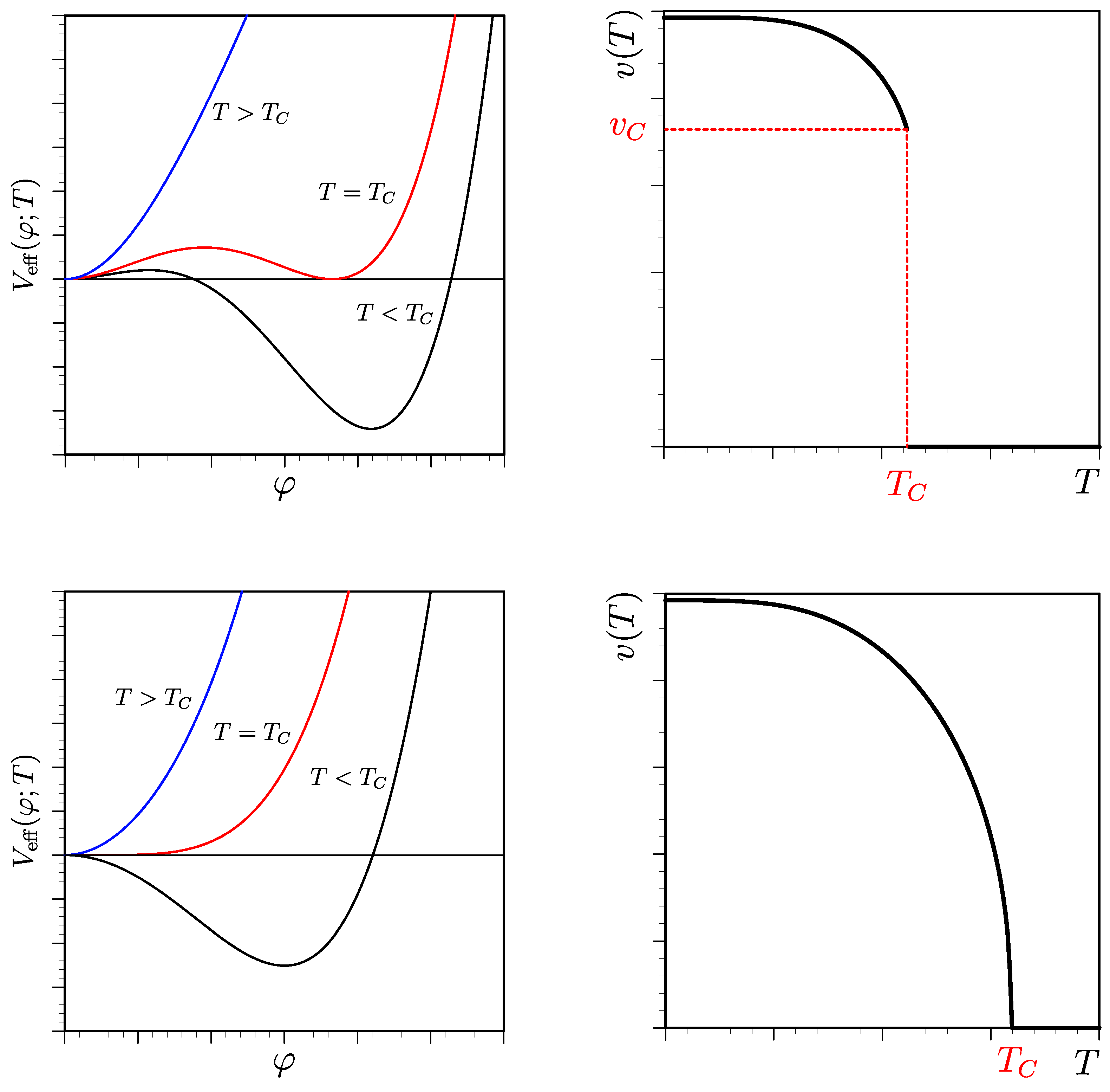
In Figure 1, first- and second-order phase transitions are depicted in upper and lower panels, respectively. In the left panels, the effective potentials are plotted as functions of while the temperature evolutions of the scalar VEV are shown in the right panels. In the first-order phase transition case, there exists discontinuity in the evolution of the vacuum and the critical temperature () is defined at a temperature at which has the degenerate minima separated by the potential barrier as shown in the upper left panel. is the VEV at , where T approaches from below. What is important here is that the bosonic thermal loop contribution has the cubic term with a negative sign, (Here we assume that such as gauge bosons or scalars in classical scale-invariant theories. In general, however, can have an extra mass parameter, for instance in the theory, , which will be discussed below) originated from the zero Matsubara frequency mode , which can induce the potential barrier. In the second-order phase transition case, on the other hand, the temperature evolution of VEV is continuous but its first derivative with respect to the temperature has the singular behavior at which is defined by the temperature at which the curvature at the origin becomes zero. Unlike the first-order phase transition, there is no potential barrier.
In gauge theories, is inherently gauge dependent. Nevertheless, it is shown that term as well as energies at stationery points are gauge-fixing parameter independent. We discuss the gauge dependence issue in detail in Section 4.3.
Before we discuss EWPT, we consider the theory in order to see the symmetry behavior at high-T. The Lagrangian is given by
where and . This model has the symmetry, , but it is spontaneously broken because of the term. The field-dependent scalar mass is derived by . The one-loop effective potential in the scheme takes the form
where with being the Euler constant. Combining this with , one finds
where and HTE is used in the second line. One can find that the symmetry can be restored at high temperature due to the positive contribution of the term. Presence of the term may signify that the phase transition could be first order with the critical temperature of if . Or, if the term can be neglected, the phase transition would be reduced to the second order with the critical temperature of . As shown in the next section, the perturbative expansion would break down at around even if . Therefore, we cannot make any conclusion about the order of the phase transition from the above potential (9). We explicitly demonstrate why the perturbative expansion is invalidated at high temperature in the next section.
Before closing this section, we address an issue of the imaginary part of the effective potential. At , would give the imaginary part if . Its sign is determined by an prescription for the propagator. Namely, , and therefore the imaginary part of in Equation (8) is [112]
In the work of E. Weinberg and A. Wu [113], the imaginary part is interpreted as a decay rate of a state. Another interpretation is given by analogy with a Schwinger effect in Ref. [114]. Note that this imaginary part would be cancelled by a counterpart arising from the thermal function of at high temperature, as indicated by Equation (9). Nevertheless, the effective potential (9) still can be complex since the term gives another imaginary part if , which could be viewed as a harbinger of the breakdown of the perturbation theory. As discussed in the next section, the term would be modified as a consequence of the thermal resummation and the imaginary part could disappear at high temperature (see Equation (25) or Equation (28)).
3. Breakdown of Perturbative Expansion and Thermal Resummation
Let us consider some loop diagrams at high temperature. For illustrative purpose, we focus on the theory [3] (for further developments that are not covered here, see, e.g., Ref. [46,115]). As is the case, the mass term receives higher-order corrections as
where is the temperature-dependent self-energy. At one-loop order, one has
where
![Symmetry 12 00733 i001]() where and . Therefore, this diagram grows with at high temperature. The second term comes from the mode, which brings about the IR divergence discussed below. Now we estimate multi-loop diagrams by fully exploiting Equation (13). For the moment, we ignore the numerical coefficients to make our discussion simpler.
where and . Therefore, this diagram grows with at high temperature. The second term comes from the mode, which brings about the IR divergence discussed below. Now we estimate multi-loop diagrams by fully exploiting Equation (13). For the moment, we ignore the numerical coefficients to make our discussion simpler.

There exist two types of the 2-loop diagrams: the figure-8 and sunset diagrams. The figure-8 diagram is composed of one 1-vertex bubble (VB) and one 2VB. The former goes like as seen from Equation (13) while the latter is estimated as , which amounts to
![Symmetry 12 00733 i002]()


Comparing those two 2-loop diagrams, one finds that the figure-8 diagram becomes dominant at high temperature. Despite this fact, the sunset diagram plays an important role in studying the phase transition [116].
Attaching one more 1VB to the lower bubble in the figure-8 diagram, one gets a mouse diagram in which 3VB comes in. This new contribution is evaluated as . Thus we have
![Symmetry 12 00733 i004]()

On the other hand, if we attach one 1 VB to the upper bubble in the figure-8 diagram, it becomes a cactus diagram, which is composed of one 1 VB and two 2 VB. From the above estimates, it follows that
![Symmetry 12 00733 i005]()

Taking the ratio of those two 3-loop diagrams, one finds that (mouse)/(cactus) = . Therefore, the mouse diagram becomes dominant at high temperature. We could have another 3-loop diagram which is made by attaching one 1 VB to the sunset diagram. However such a diagram cannot compete with the mouse diagram. Noting that whenever one 1 VB is attached to the lower bubble in the figure-8 diagram, one gets the factor of . Thus, a diagram that is composed of 1 VB and one nVB (referred to as daisy diagram) is found to be
![Symmetry 12 00733 i006]()

Therefore, in addition to , it needs in order that the perturbative expansion makes sense. However, as discussed in Section 2, one has when the symmetry is restored, which means that the one-loop order calculation is not reliable in studying the phase transition. This demonstration suggests that one has to incorporate all the relevant diagrams into our calculation, that is, necessity of the resummation.
Let us redo the above analysis taking the numerical factor with care. The daisy diagram is actually given by
where . Note that is reduced to 1VB given in Equation (13). Summing up all the dominant diagrams at high temperature, the self-energy is calculated as
Therefore, the daisy resummation to leading order amounts to
Note that the sunset-type diagrams such as (15) are not included in the daisy and super-daisy resummations. In the study of the phase transition, however, such diagram cannot be neglected.
It should be emphasized that the resummation is merely re-organization of the perturbative expansion so that original Lagrangian is not changed at all. This can be seen as follows. Following the work of Parwani [118], let us decompose the bare Lagrangian () into the renormalized one () and corresponding counterterms () and then add and subtract the thermal mass correction of as
We regard appearing in the renormalized Lagrangian as un-perturbed part while the latter as the part of the counterterm. In this resummed Lagrangian, the scalar propagator is given by with . Thus, the one-loop effective potential can be obtained by replacing with in Equation (8):
Putting all together and taking HTE, the effective potential in the Parwani scheme is reduced to
where (const) denotes the -independent terms that are irrelevant to the phase transition.
Recalling that the IR divergence is originated from the mode, we could resum only this mode (Arnold-Espinosa (AE) scheme) [116]. In this scheme, the resummed effective potential is cast into the form
where in the first line is the summation over n without mode, the first term in the second line is the same as the unresummed one-loop effective potential given in Equation (8) while the second term is the daisy resuumation, which reads
In the AE scheme, the total effective potential using HTE is cast into the form
where (const) denotes the -independent terms. This resummed potential agrees with that in the Parwani scheme Equation (25) except for the last term. Comparisons between the two resummation schemes in a model of the SM extension can be found in Ref. [75] (for a recent study, see, e.g., Ref. [119]).
Here, we make a comment on the order of the phase transition in the theory. It is known from the general argument of renormalization group analysis that the phase transition is second order [120]. In contrast to this, perturbative calculations could give a different answer. For instance, if one uses the effective potential with the daisy resummation shown here or super-daisy resummation, the phase transition is first order [117,121,122]. Beyond those resummations including the sunset-type diagrams, however, it turns into the second-order phase transition [123,124,125], which is consistent with the aforementioned general argument.
Before closing this section, we briefly discuss the resummation in gauge theories. At finite temperature, the Lorentz symmetry is broken by thermal bath specified by a four vector of , which takes the form of in the rest frame of thermal bath. Consequently, the gauge boson polarization tensor is constructed by four basis tensors . It is convenient to define such that . With those four basis tensors, is generally written as
where
Note that both and are 4-dimensionally transverse while the former (the latter) are 3-dimensionally longitudinal (transverse). In Landau gauge (), the resummed gauge boson propagator has the form
where m is the gauge boson mass at . Here, two kind of the gauge boson thermal masses are defined as
The former is called electric mass and the latter magnetic mass. It should be noted that the order of taking limits is not exchangeable. The opposite limit give different results [126]. As well known, the electric mass can arise perturbatively, which is the order of with g being a gauge coupling. However, it is proven that the magnetic mass does not arise in abelian gauge theories to all orders [126]. In non-abelian gauge theories, on the other hand, the magnetic mass can be generated though its evaluation requires non-perturbative methods [127]. Unlike the electric mass, the order of the magnetic mass is .
Thermal resummation in non-abelian gauge theories is formulated as Hard Thermal Loop (HTL) perturbation theory [128,129,130,131], which can resum leading corrections in a gauge-invariant way. This method has been applied to quantum chromodynamics (QCD). In EW theories, on the other hand, there exist additional mass scales coming from the Higgs and/or new particles beyond the SM, and thus the presumed scale hierarchy in HTL does not always hold. In this article, we do not cover details of HTL and other related topics, and readers are referred to Refs. [126,127,132,133,134,135,136].
4. Electroweak Phase Transition
The discovery of the Higgs boson in 2012 has completed the particle content of the SM, and its mass measurement is the first step towards the re-construction of the Higgs potential. In order to confirm the role of the Higgs boson as the EW symmetry breaker, the measurement of the Higgs self-coupling is indispensable. For the detectability at future high-energy colliders, see, e.g., Refs. [137,138,139]. As discussed in the previous section, the symmetry can be restored at high temperature, implying that EWPT can occur at early epoch of the Universe. If this is the case, a question of our interest is how it takes place, i.e., what is the order of EWPT? In this section, we discuss a case of first-order EWPT, which is a dramatic event for cosmology. We exemplify a case in which intermediate breaking of a symmetry at finite temperature plays a pivotal role in realizing the first-order EWPT.
4.1. Standard Model
We start by discussing EWPT in the SM. Tree-level Higgs potential is comprised of the following two gauge-invariant terms:
where and are presumed. We denote the Higgs doublet field with a hypercharge 1/2 as
where GeV, h denotes the Higgs boson with a mass of 125 GeV, and are the Nambu-Goldstone (NG) bosons that are absorbed into the longitudinal components of the Z and bosons. The vacuum is determined by the stationary condition of
where denotes X is evaluated in the vacuum where the fluctuation fields are zero, enforcing . In the vacuum, the Higgs boson mass is given by
where the vacuum condition is used to eliminate .
Let us denote the classical constant background field as . From Equation (34), the tree-level effective potential is given by
As is the calculation in the theory, the one-loop effective potential without thermal resummation is written as
with
where , is regularized by the scheme, are the degrees of freedom with a statistics: , , , and . for scalars and fermions while for gauge bosons. The explicit forms of the field-dependent masses are
where , and are the , and top Yukawa couplings, respectively. The masses in the vacuum are obtained by .
The vacuum and Higgs boson mass at one-loop level in the scheme are defined by the conditions:
Note that the relationship between the Higgs boson mass and the on-shell (OS) mass () is given by
where with being the self-energy of the Higgs boson regularized by the scheme. Note that all the parameters except in Equation (45) are the running parameters that are governed by renormalization group equations. One can show that is independent of by noting that
where is the anomalous dimension of the Higgs field. At one-loop order, we actually have
where is given by Equation (44), and . From those, it follows that at one-loop level.
We note in passing that in the SM, the one-loop correction of is rather minor if is evaluated at the pole mass of the top quark.
Another renormalization conditions often used in the literature is “OS-like" renormalization in which [5,75]
where . Those two conditions determine and as
where is used in . With those, the effective potential at one-loop level takes the form
Note that this scheme is not exactly the same as the OS scheme since the mass is not defined at the pole position of the Higgs boson propagator as given above. By “OS-like", we mean that tree-level relations among the model parameters such as hold even at higher orders as is the genuine OS renormalization. We quantify numerical impacts of the scheme dependences on EWPT in Section 4.4. In what follows, we employ the OS-like scheme.
Aside from numerical accuracy, HTEs of make it easy to discuss physics. The high-T expanded effective potential is cast into the form
where
Appearance of the cubic term signals that EWPT is first order. Its critical temperature satisfies
from which, one gets
Note that due to the presence of E. In the case of second-order EWPT in which , becomes the critical temperature. Straightforward numerical calculations show that GeV, , , and , which leads to GeV and GeV, where GeV, GeV, GeV and GeV are used [6].
In the context of EWBG, to avoid the washout of the created BAU after EWPT, one has to have
However, from the above numerical analysis one has . Therefore, the EWBG possibility is excluded in the SM. We note in passing that if the Higgs boson is the free parameter and other particles masses are fixed to the observed values, one finds . To circumvent this difficulty, enhanced E and/or suppressed are necessary. This can be realized in the extension of the SM, as discussed in the next section.
Before moving to beyond the SM, we give some remarks on the above results.
- The above demonstration does not take the thermal resummation into consideration. If one performs it by either the Parwani or AE scheme, E would be diminished by the resummation effect as discussed in Section 3.
- The effective potential is the sum of 1-particle-irreducible diagrams by definition, which is inherently gauge dependent, and so the VEV defined by the minimum of the effective potential depends on a choice of specific gauge. This is natural consequence since the normalization of the scalar fields (wavefunction renormalization) is missing. Notwithstanding, energies at stationary points are gauge independent obeyed by the NFK identity [109,110].
- Since the phase transition is generically non-perturbative phenomenon, lattice calculations are more suitable to obtain robust results. It is shown in Refs. [140,141,142,143] that EWPT turns into smooth crossover for GeV. After the Higgs boson discovery, EWPT is re-analyzed in Ref. [144] in a different context. The “critical temperature" is found to be GeV.
4.2. Standard Model with a Real Scalar
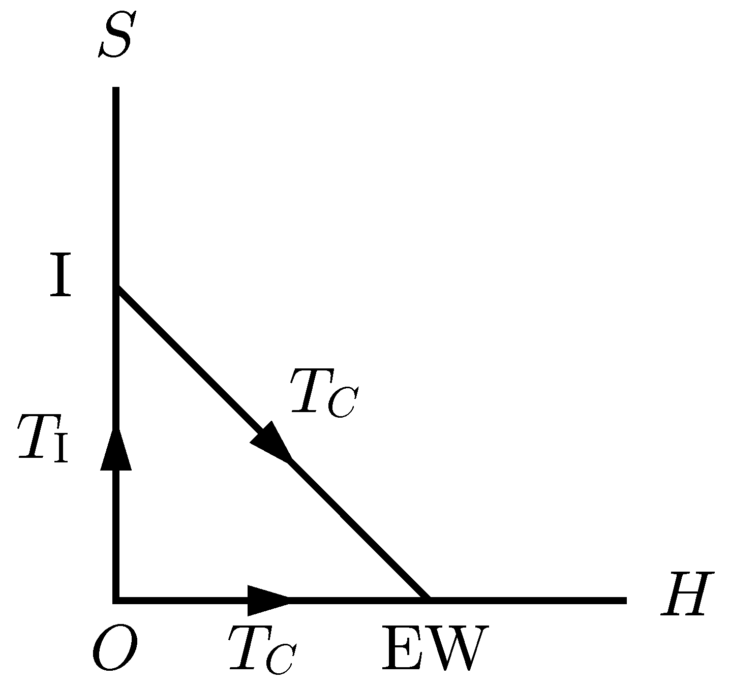
As discussed in the previous section, the parameter space of the strong first-order EWPT () in the SM is not consistent with the observed Higgs boson. One of the simplest extensions of the SM is to add a real scalar field that is singlet under the SM gauge group (referred to as rSM). As first emphasized by Funakubo et al. in the next-to-minimal supersymmetric SM [97], such a singlet scalar can increase the possibility of the first-order EWPT owing to multi-step transitions. In addition to this, the singlet scalar can be DM if the model is symmetric. (The symmetry is phenomenologically introduced to have the DM candidate. Since its origin is highly model dependent, we do not specify it in this review). Note that even though the symmetry is preserved at , it does not necessarily hold at depending on thermal history of the vacuum evolution. In what follows, we discuss two types of phase transitions as shown in Figure 2.
Let us denote the singlet scalar as S. The extended Higgs potential is cast into the form
where H is given in Equation (35). The stationary conditions of H and S are, respectively, given by
where is VEV of S. By assumption, the symmetry is preserved at , which enforces . The Higgs boson masses at tree level take the form
Denoting the classical constant background fields of the doublet and singlet scalars as and , the effective potential at tree level is given by
To avoid the unbounded from below in the and directions, and are imposed. Moreover, the case of needs additional condition. Denoting with being a real parameter, the quartic terms in the Higgs potential can be written as
The coefficient of has to be positive for any , which leads to .
For , a local minimum can appear in the singlet scalar direction, developing . For the EW vacuum to be the global minimum, one must have , resulting in
In the rSM, only 3 free parameters exist. We consider , and as the input parameters in the following discussion.
First, we consider a simplified potential
where and are the thermal masses of H and S, which are, respectively, given by [32]
We begin with discussing a case in which the phase transition occurs only once (1-step transition scenario). It is convenient that the two scalar fields are parametrized in polar coordinates: and , where . Hereafter we use shorthand notations: and . At , one finds that with being , yielding
Therefore, the strength of the first-order EWPT can be enhanced for .
Now we move on to discuss another case in which the phase transitions occur twice (2-step transition scenario). In this case, the phase transition prior to EWPT can be described by the potential
The local minimum appears if , which is given by . Note that the critical temperature in this case (denoted as ) is given by , i.e.,
To analyze EWPT, we use the polar coordinates and . Repeating the similar calculation as the case of the 1-step transition scenario, one can find
Owing to SSB of the symmetry, additional terms proportional to appear in the numerator. Consequently, the first-order EWPT can be strengthened if together with , which is stark contrast to the 1-step transition scenario. Note that while can get larger for smaller as shown above, the smallness of is limited by the global minimum condition (67).
Without the simplification, the one-loop effective potential in the scheme is given by
where . In the numerical study shown in Section 4.4, we adopt the Parwani scheme for the thermal resummation.
4.3. Perturbative Gauge-Invariant Treatment for the Thermal Phase Transitions
As briefly discussed in Section 4.1, the treatment of EWPT shown above suffers from the gauge dependence problem. Here, we introduce two gauge-invariant methods: high-T potential (HT) scheme and Patel-Ramsey-Musolf (PRM) scheme [145] and apply them to the 2-step transition scenario in the rSM.
Given the fact that the leading thermal mass is gauge independent, the simplest gauge-invariant effective potential is constructed by adding the thermal quadratic terms into the tree-level Higgs potential, which is nothing but the potential (68) without the cubic term:
In this method, the 1-step scenario always induces the second-order EWPT while the 2-step transition scenario could accommodate the first-order EWPT depending on the parameter choices, as understood from the analysis in Section 4.2. In spite of the gauge-invariant construction, the main drawback here is lack of the quantum corrections that could be relevant. We quantify this statement in Section 4.4.
In contrast to this, the PRM scheme can take account of the quantum corrections to based on the NFK identity. The statement of this identity is that energies at stationary points of the effective potential are gauge independent, i.e.,
where is the gauge-fixing parameter and is some functional. While the statement is very simple, it needs some caution when we work in the perturbation theory. To derive the NFK identity at given order, we expand and in powers of ℏ as
At tree level, there is no dependence so that must vanish. At one-loop level, , on other hand, one can find
It should be noted that the dependence of vanishes at the stationary points of rather than . Let us look into the dependence of more explicitly. The one-loop effective potential in the gauge may contain the following -dependent pieces:
where and are the field-dependent masses of the gauge and NG bosons. The dependence would disappear at the point of , namely, , satisfying the NFK identity at one-loop order. On the other hand, the vacuum condition used in the usual perturbative analysis, for example in the scheme, is as given in Equation (43), which thus leads to the -dependent result.
In the PRM scheme in the rSM, at one-loop level is determined by the degeneracy condition
where GeV, and is the minimum of . Unlike the usual condition of , the field values are fixed to their tree-level minima at . Since , where and are the one-loop level minima, in the PRM tends to be lower than that in the ordinary case, which can increase . As for the determination of in the PRM scheme, on the other hand, the HT potential (76) is used to maintain the gauge invariance.
Here we remark the thermal resummation in the PRM scheme. While the resumamtion can be implemented in a gauge-invariant way [145], it needs the two-loop effective potential for the consistency of the calculation. Nevertheless, such a calculation is not available in the literature and hence beyond the scope of this review article.
4.4. Comparisons among Various Calculation Schemes
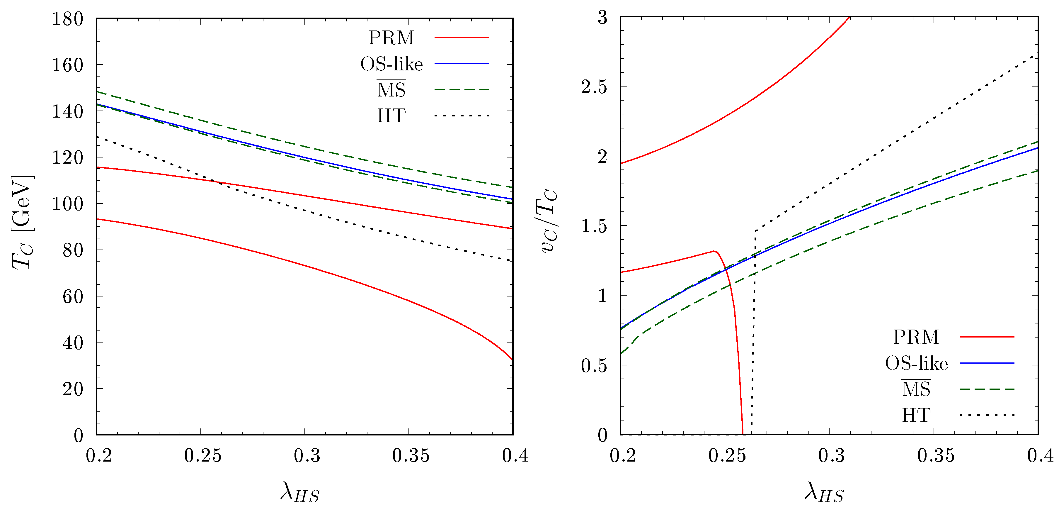
Now we conduct numerical analysis [56]. Among the three input parameters , we take , which is consistent with DM physics [146,147], and [37], where is determined by the vacuum condition given in Equation (67). is taken as the varying parameter. In Figure 3, numerical results of EWPT in rSM are summarized. In order to see the gauge and scale dependences on EWPT, we consider four calculations methods: the OS-like and schemes as the gauge-dependent methods while PRM and HT as the gauge-independent ones. In the left panel, is shown as a function of . As for the PRM and schemes, we take . One can see that all the results show the same behavior, namely, gets decreased as increases, which is the fact that the larger make the vacuum energy of I phase lower so that the degeneracy with that of EW phase happen at lower temperature. As seen, OS-like and schemes agree with each other nicely, while the other two gauge-invariant methods give lower to some extent. For PRM, this behavior is the expected consequence as discussed above. The reason why the dependence in PRM is larger than that in the scheme is that the one-loop minimization condition is used in the latter case, which can partially cancel the dependence in determining , while such a cancellation is missing due to use of the tree-level minimization condition in the former case [56].
In the right panel, are plotted in the four cases. The color schemes are the same as in the left plot. The OS-like and schemes are consistent with each other within the scale uncertainties. On the other hand, the PRM scheme show the rather large scale uncertainties. As seen, becomes zero for , which is due to the fact that in PRM gets larger than that in the HT scheme as shown in the left plot. Although somewhat big discrepancy exists among the gauge-dependent and independent schemes, we expect that it gets ameliorated when the higher-order corrections such as the daisy resummation as well as the two-loop corrections are incorporated in the PRM scheme.
5. Summary and Outlook
We have discussed the high temperature behaviors of symmetries using the perturbative effective potential. As explicitly demonstrated in the theory, the symmetry restoration generically causes the IR divergence problem that invalidates the ordinary perturbative expansion at zero temperature. To cure this problem, the dominant temperature corrections must be resummed in a consistent way. In this review, we introduce the two common methods of the thermal resummations, i.e., Parwani and Arnold-Espinosa schemes. In the former all the Matsubara frequency modes are resummed while in the latter only zero mode is resummed.
As an interesting cosmological application, we discussed EWPT focusing on the first-order phase transition case, which is motivated by EWBG as well as physics of gravitational waves. For illustration, the real scalar extended SM with the symmetry is considered. In this model, the breaking of the symmetry at finite temperature can increase the possibility of the first-order EWPT and its restoration at zero temperature plays a fundamental role in accommodating the DM candidate.
We also addressed the problem of gauge and scheme dependences of EWPT. The comparison is made among the four calculation methods: , OS-like, PRM and HT schemes. In any case, the numerical study shows that the behaviors of the critical temperature against the coupling between the SM Higgs and real scalar are consistent with each other and indicates the occurrence of the first-order EWPT (for the PRM scheme within the scale uncertainties). Nevertheless, none of the methods are gauge invariant and less scale dependent, which motivates one to refine the calculations including higher-order corrections.
In closing, through the demonstration here, we highlight the technical issues of the perturbative treatments of the thermal phase transition and illustrate the need to exercise caution when applying them to EWPT. However, this does not necessarily mean that the issues are just technical. In the current perturbative approach, for instance, the order parameter is the VEV of the Higgs field which is inherently gauge dependent. We may need to find better order parameter and newly develop formalism rather than fixing the drawbacks of the current methods.
Funding
This research received no external funding.
Acknowledgments
I would like to thank all my collaborators for fruitful discussions.
Conflicts of Interest
The author declares no conflict of interest.
Appendix A. Thermally Corrected Field-Dependent Masses in the rSM
The thermally corrected Higgs mass matrix takes the form
where and are given by Equations (69) and (70). For the NG bosons, one finds
As given in Equation (33), there are two distinct thermal masses for the longitudinal and transverse gauge fields. At one-loop order, only the former receive the nonzero corrections. The thermally corrected gauge boson mass matrix in the basis is cast into the form
The corresponding eigenvalues are, respectively, given by
where and are [148]
where denotes the number of fermion generation and is the number of color, and the last equalities are evaluated with .
References
- Kirzhnits, D.A. Weinberg model in the hot universe. JETP Lett. 1972, 15, 529–531. [Google Scholar]
- Kirzhnits, D.A.; Linde, A.D. Macroscopic Consequences of the Weinberg Model. Phys. Lett. 1972, 42B, 471–474. [Google Scholar] [CrossRef]
- Dolan, L.; Jackiw, R. Symmetry Behavior at Finite Temperature. Phys. Rev. 1974, D9, 3320–3341. [Google Scholar] [CrossRef]
- Weinberg, S. Gauge and Global Symmetries at High Temperature. Phys. Rev. 1974, D9, 3357–3378. [Google Scholar] [CrossRef]
- Kirzhnits, D.A.; Linde, A.D. Symmetry Behavior in Gauge Theories. Ann. Phys. 1976, 101, 195–238. [Google Scholar] [CrossRef]
- Particle Data Group. Review of Particle Physics. Phys. Rev. 2018, D98, 030001. [Google Scholar] [CrossRef] [Green Version]
- Kuzmin, V.A.; Rubakov, V.A.; Shaposhnikov, M.E. On the Anomalous Electroweak Baryon Number Nonconservation in the Early Universe. Phys. Lett. 1985, 155B, 36. [Google Scholar] [CrossRef]
- Rubakov, V.A.; Shaposhnikov, M.E. Electroweak baryon number nonconservation in the early universe and in high-energy collisions. Usp. Fiz. Nauk 1996, 166, 493–537. [Google Scholar] [CrossRef] [Green Version]
- Funakubo, K. CP violation and baryogenesis at the electroweak phase transition. Prog. Theor. Phys. 1996, 96, 475–520. [Google Scholar] [CrossRef]
- Riotto, A. Theories of baryogenesis. In Proceedings of the Summer School in High-energy physics and cosmology, Trieste, Italy, 29 June–17 July 1998; pp. 326–436. [Google Scholar]
- Quiros, M. Finite temperature field theory and phase transitions. In Proceedings of the Summer School in High-Energy Physics and Cosmology, Trieste, Italy, 29 June–17 July 1998; pp. 187–259. [Google Scholar]
- Trodden, M. Electroweak baryogenesis. Rev. Mod. Phys. 1999, 71, 1463–1500. [Google Scholar] [CrossRef] [Green Version]
- Bernreuther, W. CP violation and baryogenesis. Lect. Notes Phys. 2002, 591, 237–293. [Google Scholar]
- Cline, J.M. Baryogenesis. In Proceedings of the Les Houches Summer School - Session 86: Particle Physics and Cosmology: The Fabric of Spacetime Les Houches, Les Houches, France, 31 July–25 August 2006. [Google Scholar]
- Morrissey, D.E.; Ramsey-Musolf, M.J. Electroweak baryogenesis. New J. Phys. 2012, 14, 125003. [Google Scholar] [CrossRef]
- Konstandin, T. Quantum Transport and Electroweak Baryogenesis. Phys. Usp. 2013, 56, 747–771. [Google Scholar] [CrossRef]
- Caprini, C.; Hindmarsh, M.; Huber, S.; Konstandin, T.; Kozaczuk, J.; Nardini, G.; No, J.M.; Petiteau, A.; Schwaller, P.; Servant, G.; et al. Science with the space-based interferometer eLISA. II: Gravitational waves from cosmological phase transitions. JCAP 2016, 1604, 001. [Google Scholar] [CrossRef]
- Choi, J.; Volkas, R.R. Real Higgs singlet and the electroweak phase transition in the Standard Model. Phys. Lett. 1993, B317, 385–391. [Google Scholar] [CrossRef] [Green Version]
- Ham, S.W.; Jeong, Y.S.; Oh, S.K. Electroweak phase transition in an extension of the standard model with a real Higgs singlet. J. Phys. 2005, G31, 857–871. [Google Scholar] [CrossRef] [Green Version]
- Ahriche, A. What is the criterion for a strong first order electroweak phase transition in singlet models? Phys. Rev. 2007, D75, 083522. [Google Scholar] [CrossRef] [Green Version]
- Espinosa, J.R.; Quiros, M. Novel Effects in Electroweak Breaking from a Hidden Sector. Phys. Rev. 2007, D76, 076004. [Google Scholar] [CrossRef] [Green Version]
- Das, S.; Fox, P.J.; Kumar, A.; Weiner, N. The Dark Side of the Electroweak Phase Transition. JHEP 2010, 11, 108. [Google Scholar] [CrossRef] [Green Version]
- Chung, D.J.H.; Long, A.J. Cosmological Constant, Dark Matter, and Electroweak Phase Transition. Phys. Rev. 2011, D84, 103513. [Google Scholar] [CrossRef] [Green Version]
- Espinosa, J.R.; Gripaios, B.; Konstandin, T.; Riva, F. Electroweak Baryogenesis in Non-minimal Composite Higgs Models. JCAP 2012, 1201, 012. [Google Scholar] [CrossRef]
- Cline, J.M.; Kainulainen, K. Electroweak baryogenesis and dark matter from a singlet Higgs. JCAP 2013, 1301, 012. [Google Scholar] [CrossRef]
- Fairbairn, M.; Hogan, R. Singlet Fermionic Dark Matter and the Electroweak Phase Transition. JHEP 2013, 09, 022. [Google Scholar] [CrossRef] [Green Version]
- Cline, J.M.; Kainulainen, K.; Scott, P.; Weniger, C. Update on scalar singlet dark matter. Phys. Rev. 2013, D88, 055025. [Google Scholar] [CrossRef] [Green Version]
- Damgaard, P.H.; O’Connell, D.; Petersen, T.C.; Tranberg, A. Constraints on New Physics from Baryogenesis and Large Hadron Collider Data. Phys. Rev. Lett. 2013, 111, 221804. [Google Scholar] [CrossRef] [Green Version]
- Li, T.; Zhou, Y.F. Strongly first order phase transition in the singlet fermionic dark matter model after LUX. JHEP 2014, 07, 006. [Google Scholar] [CrossRef] [Green Version]
- Profumo, S.; Ramsey-Musolf, M.J.; Shaughnessy, G. Singlet Higgs phenomenology and the electroweak phase transition. JHEP 2007, 08, 010. [Google Scholar] [CrossRef] [Green Version]
- Ashoorioon, A.; Konstandin, T. Strong electroweak phase transitions without collider traces. JHEP 2009, 07, 086. [Google Scholar] [CrossRef] [Green Version]
- Espinosa, J.R.; Konstandin, T.; Riva, F. Strong Electroweak Phase Transitions in the Standard Model with a Singlet. Nucl. Phys. 2012, B854, 592–630. [Google Scholar] [CrossRef]
- Fuyuto, K.; Senaha, E. Improved sphaleron decoupling condition and the Higgs coupling constants in the real singlet-extended standard model. Phys. Rev. 2014, D90, 015015. [Google Scholar] [CrossRef] [Green Version]
- Alanne, T.; Tuominen, K.; Vaskonen, V. Strong phase transition, dark matter and vacuum stability from simple hidden sectors. Nucl. Phys. 2014, B889, 692–711. [Google Scholar] [CrossRef] [Green Version]
- Profumo, S.; Ramsey-Musolf, M.J.; Wainwright, C.L.; Winslow, P. Singlet-catalyzed electroweak phase transitions and precision Higgs boson studies. Phys. Rev. 2015, D91, 035018. [Google Scholar] [CrossRef] [Green Version]
- Craig, N.; Lou, H.K.; McCullough, M.; Thalapillil, A. The Higgs Portal Above Threshold. JHEP 2016, 02, 127. [Google Scholar] [CrossRef] [Green Version]
- Curtin, D.; Meade, P.; Yu, C.T. Testing Electroweak Baryogenesis with Future Colliders. JHEP 2014, 11, 127. [Google Scholar] [CrossRef] [Green Version]
- Kozaczuk, J. Bubble Expansion and the Viability of Singlet-Driven Electroweak Baryogenesis. JHEP 2015, 10, 135. [Google Scholar] [CrossRef] [Green Version]
- Damgaard, P.H.; Haarr, A.; O’Connell, D.; Tranberg, A. Effective Field Theory and Electroweak Baryogenesis in the Singlet-Extended Standard Model. JHEP 2016, 02, 107. [Google Scholar] [CrossRef] [Green Version]
- Ghosh, S.; Kundu, A.; Ray, S. Potential of a singlet scalar enhanced Standard Model. Phys. Rev. 2016, D93, 115034. [Google Scholar] [CrossRef] [Green Version]
- Kotwal, A.V.; Ramsey-Musolf, M.J.; No, J.M.; Winslow, P. Singlet-catalyzed electroweak phase transitions in the 100 TeV frontier. Phys. Rev. 2016, D94, 035022. [Google Scholar] [CrossRef] [Green Version]
- Chala, M.; Nardini, G.; Sobolev, I. Unified explanation for dark matter and electroweak baryogenesis with direct detection and gravitational wave signatures. Phys. Rev. 2016, D94, 055006. [Google Scholar] [CrossRef] [Green Version]
- Tenkanen, T.; Tuominen, K.; Vaskonen, V. A Strong Electroweak Phase Transition from the Inflaton Field. JCAP 2016, 1609, 037. [Google Scholar] [CrossRef]
- Huang, P.; Long, A.J.; Wang, L.T. Probing the Electroweak Phase Transition with Higgs Factories and Gravitational Waves. Phys. Rev. 2016, D94, 075008. [Google Scholar] [CrossRef] [Green Version]
- Vaskonen, V. Electroweak baryogenesis and gravitational waves from a real scalar singlet. Phys. Rev. 2017, D95, 123515. [Google Scholar] [CrossRef] [Green Version]
- Curtin, D.; Meade, P.; Ramani, H. Thermal Resummation and Phase Transitions. Eur. Phys. J. 2018, C78, 787. [Google Scholar] [CrossRef]
- Cline, J.M.; Kainulainen, K.; Tucker-Smith, D. Electroweak baryogenesis from a dark sector. Phys. Rev. 2017, D95, 115006. [Google Scholar] [CrossRef] [Green Version]
- Beniwal, A.; Lewicki, M.; Wells, J.D.; White, M.; Williams, A.G. Gravitational wave, collider and dark matter signals from a scalar singlet electroweak baryogenesis. JHEP 2017, 08, 108. [Google Scholar] [CrossRef] [Green Version]
- Ghorbani, P.H. Electroweak Baryogenesis and Dark Matter via a Pseudoscalar vs. Scalar. JHEP 2017, 08, 058. [Google Scholar] [CrossRef]
- Marzola, L.; Racioppi, A.; Vaskonen, V. Phase transition and gravitational wave phenomenology of scalar conformal extensions of the Standard Model. Eur. Phys. J. 2017, C77, 484. [Google Scholar] [CrossRef] [Green Version]
- Chen, C.Y.; Kozaczuk, J.; Lewis, I.M. Non-resonant Collider Signatures of a Singlet-Driven Electroweak Phase Transition. JHEP 2017, 08, 096. [Google Scholar] [CrossRef]
- Kurup, G.; Perelstein, M. Dynamics of Electroweak Phase Transition In Singlet-Scalar Extension of the Standard Model. Phys. Rev. 2017, D96, 015036. [Google Scholar] [CrossRef] [Green Version]
- Jain, B.; Lee, S.J.; Son, M. Validity of the effective potential and the precision of Higgs field self-couplings. Phys. Rev. 2018, D98, 075002. [Google Scholar] [CrossRef] [Green Version]
- Ghorbani, K.; Ghorbani, P.H. Strongly First-Order Phase Transition in Real Singlet Scalar Dark Matter Model. J. Phys. 2020, G47, 015201. [Google Scholar] [CrossRef] [Green Version]
- Huang, F.P.; Qian, Z.; Zhang, M. Exploring dynamical CP violation induced baryogenesis by gravitational waves and colliders. Phys. Rev. 2018, D98, 015014. [Google Scholar] [CrossRef] [Green Version]
- Chiang, C.W.; Li, Y.T.; Senaha, E. Revisiting electroweak phase transition in the standard model with a real singlet scalar. Phys. Lett. 2019, B789, 154–159. [Google Scholar] [CrossRef]
- Beniwal, A.; Lewicki, M.; White, M.; Williams, A.G. Gravitational waves and electroweak baryogenesis in a global study of the extended scalar singlet model. JHEP 2019, 02, 183. [Google Scholar] [CrossRef] [Green Version]
- Carena, M.; Liu, Z.; Wang, Y. Electroweak Phase Transition with Spontaneous Z2-Breaking. 2019. Available online: http://xxx.lanl.gov/abs/1911.10206 (accessed on 20 April 2020).
- Kondo, Y.; Umemura, I.; Yamamoto, K. First order phase transition in the singlet Majoron model. Phys. Lett. 1991, B263, 93–96. [Google Scholar] [CrossRef]
- Espinosa, J.R.; Quiros, M. The Electroweak phase transition with a singlet. Phys. Lett. 1993, B305, 98–105. [Google Scholar] [CrossRef] [Green Version]
- Benson, K.E.C. Avoiding baryon washout in the extended Standard Model. Phys. Rev. 1993, D48, 2456–2461. [Google Scholar] [CrossRef]
- Cline, J.M.; Laporte, G.; Yamashita, H.; Kraml, S. Electroweak Phase Transition and LHC Signatures in the Singlet Majoron Model. JHEP 2009, 07, 040. [Google Scholar] [CrossRef]
- Farzinnia, A.; Ren, J. Strongly First-Order Electroweak Phase Transition and Classical Scale Invariance. Phys. Rev. 2014, D90, 075012. [Google Scholar] [CrossRef] [Green Version]
- Chao, W. First order electroweak phase transition triggered by the Higgs portal vector dark matter. Phys. Rev. 2015, D92, 015025. [Google Scholar] [CrossRef] [Green Version]
- Kang, Z.; Ko, P.; Matsui, T. Strong first order EWPT & strong gravitational waves in Z3-symmetric singlet scalar extension. JHEP 2018, 02, 115. [Google Scholar] [CrossRef] [Green Version]
- Chiang, C.W.; Ramsey-Musolf, M.J.; Senaha, E. Standard Model with a Complex Scalar Singlet: Cosmological Implications and Theoretical Considerations. Phys. Rev. 2018, D97, 015005. [Google Scholar] [CrossRef] [Green Version]
- Cheng, W.; Bian, L. From inflation to cosmological electroweak phase transition with a complex scalar singlet. Phys. Rev. 2018, D98, 023524. [Google Scholar] [CrossRef] [Green Version]
- Grzadkowski, B.; Huang, D. Spontaneous CP-Violating Electroweak Baryogenesis and Dark Matter from a Complex Singlet Scalar. JHEP 2018, 08, 135. [Google Scholar] [CrossRef] [Green Version]
- Chen, N.; Li, T.; Wu, Y.; Bian, L. Discriminate the Discrete Symmetry Through the Future e+e- Colliders and Gravitational Waves. 2019. Available online: http://xxx.lanl.gov/abs/1911.05579 (accessed on 20 April 2020).
- Bochkarev, A.I.; Kuzmin, S.V.; Shaposhnikov, M.E. Electroweak baryogenesis and the Higgs boson mass problem. Phys. Lett. 1990, B244, 275–278. [Google Scholar] [CrossRef]
- Turok, N.; Zadrozny, J. Phase transitions in the two doublet model. Nucl. Phys. 1992, B369, 729–742. [Google Scholar] [CrossRef]
- Land, D.; Carlson, E.D. Two stage phase transition in two Higgs models. Phys. Lett. 1992, B292, 107–112. [Google Scholar] [CrossRef] [Green Version]
- Hammerschmitt, A.; Kripfganz, J.; Schmidt, M.G. Baryon asymmetry from a two stage electroweak phase transition? Z. Phys. 1994, C64, 105–110. [Google Scholar] [CrossRef]
- Funakubo, K.; Kakuto, A.; Takenaga, K. The Effective potential of electroweak theory with two massless Higgs doublets at finite temperature. Prog. Theor. Phys. 1994, 91, 341–352. [Google Scholar] [CrossRef]
- Cline, J.M.; Lemieux, P.A. Electroweak phase transition in two Higgs doublet models. Phys. Rev. 1997, D55, 3873–3881. [Google Scholar] [CrossRef] [Green Version]
- Kanemura, S.; Okada, Y.; Senaha, E. Electroweak baryogenesis and quantum corrections to the triple Higgs boson coupling. Phys. Lett. 2005, B606, 361–366. [Google Scholar] [CrossRef] [Green Version]
- Fromme, L.; Huber, S.J.; Seniuch, M. Baryogenesis in the two-Higgs doublet model. JHEP 2006, 11, 038. [Google Scholar] [CrossRef]
- Chowdhury, T.A.; Nemevsek, M.; Senjanovic, G.; Zhang, Y. Dark Matter as the Trigger of Strong Electroweak Phase Transition. JCAP 2012, 1202, 029. [Google Scholar] [CrossRef] [Green Version]
- Borah, D.; Cline, J.M. Inert Doublet Dark Matter with Strong Electroweak Phase Transition. Phys. Rev. 2012, D86, 055001. [Google Scholar] [CrossRef] [Green Version]
- Gil, G.; Chankowski, P.; Krawczyk, M. Inert Dark Matter and Strong Electroweak Phase Transition. Phys. Lett. 2012, B717, 396–402. [Google Scholar] [CrossRef] [Green Version]
- Cline, J.M.; Kainulainen, K. Improved Electroweak Phase Transition with Subdominant Inert Doublet Dark Matter. Phys. Rev. 2013, D87, 071701. [Google Scholar] [CrossRef] [Green Version]
- Dorsch, G.C.; Huber, S.J.; No, J.M. A strong electroweak phase transition in the 2HDM after LHC8. JHEP 2013, 10, 029. [Google Scholar] [CrossRef] [Green Version]
- Dorsch, G.C.; Huber, S.J.; Mimasu, K.; No, J.M. Echoes of the Electroweak Phase Transition: Discovering a second Higgs doublet through A0 → ZH0. Phys. Rev. Lett. 2014, 113, 211802. [Google Scholar] [CrossRef] [Green Version]
- Blinov, N.; Profumo, S.; Stefaniak, T. The Electroweak Phase Transition in the Inert Doublet Model. JCAP 2015, 1507, 028. [Google Scholar] [CrossRef]
- Fuyuto, K.; Senaha, E. Sphaleron and critical bubble in the scale invariant two Higgs doublet model. Phys. Lett. 2015, B747, 152–157. [Google Scholar] [CrossRef] [Green Version]
- Basler, P.; Mühlleitner, M.; Wittbrodt, J. The CP-Violating 2HDM in Light of a Strong First Order Electroweak Phase Transition and Implications for Higgs Pair Production. JHEP 2018, 03, 061. [Google Scholar] [CrossRef] [Green Version]
- Huang, F.P.; Senaha, E. Enhanced Z boson decays as a new probe of first-order electroweak phase transition at future lepton colliders. Phys. Rev. 2019, D100, 035014. [Google Scholar] [CrossRef] [Green Version]
- Wang, X.; Huang, F.P.; Zhang, X. Gravitational wave and collider signals in complex two-Higgs doublet model with dynamical CP-violation at finite temperature. Phys. Rev. 2020, D101, 015015. [Google Scholar] [CrossRef] [Green Version]
- Pietroni, M. The Electroweak phase transition in a nonminimal supersymmetric model. Nucl. Phys. 1993, B402, 27–45. [Google Scholar] [CrossRef] [Green Version]
- Espinosa, J.R.; Quiros, M.; Zwirner, F. On the electroweak phase transition in the minimal supersymmetric Standard Model. Phys. Lett. 1993, B307, 106–115. [Google Scholar] [CrossRef] [Green Version]
- Brignole, A.; Espinosa, J.R.; Quiros, M.; Zwirner, F. Aspects of the electroweak phase transition in the minimal supersymmetric standard model. Phys. Lett. 1994, B324, 181–191. [Google Scholar] [CrossRef] [Green Version]
- Davies, A.T.; Froggatt, C.D.; Moorhouse, R.G. Electroweak baryogenesis in the next-to-minimal supersymmetric model. Phys. Lett. 1996, B372, 88–94. [Google Scholar] [CrossRef] [Green Version]
- Espinosa, J.R. Dominant two loop corrections to the MSSM finite temperature effective potential. Nucl. Phys. 1996, B475, 273–292. [Google Scholar] [CrossRef] [Green Version]
- De Carlos, B.; Espinosa, J.R. The Baryogenesis window in the MSSM. Nucl. Phys. 1997, B503, 24–54. [Google Scholar] [CrossRef] [Green Version]
- Huber, S.J.; Schmidt, M.G. Electroweak baryogenesis: Concrete in a SUSY model with a gauge singlet. Nucl. Phys. 2001, B606, 183–230. [Google Scholar] [CrossRef] [Green Version]
- Funakubo, K.; Tao, S.; Toyoda, F. CP violation in the Higgs sector and phase transition in the MSSM. Prog. Theor. Phys. 2003, 109, 415–432. [Google Scholar] [CrossRef] [Green Version]
- Funakubo, K.; Tao, S.; Toyoda, F. Phase transitions in the NMSSM. Prog. Theor. Phys. 2005, 114, 369–389. [Google Scholar] [CrossRef] [Green Version]
- Huber, S.J.; Konstandin, T.; Prokopec, T.; Schmidt, M.G. Electroweak Phase Transition and Baryogenesis in the nMSSM. Nucl. Phys. 2006, B757, 172–196. [Google Scholar] [CrossRef] [Green Version]
- Funakubo, K.; Senaha, E. Electroweak phase transition, critical bubbles and sphaleron decoupling condition in the MSSM. Phys. Rev. 2009, D79, 115024. [Google Scholar] [CrossRef] [Green Version]
- Chiang, C.W.; Senaha, E. Electroweak phase transitions in the secluded U(1)-prime-extended MSSM. JHEP 2010, 06, 030. [Google Scholar] [CrossRef] [Green Version]
- Chung, D.J.H.; Long, A.J. Electroweak Phase Transition in the munuSSM. Phys. Rev. 2010, D81, 123531. [Google Scholar] [CrossRef] [Green Version]
- Kanemura, S.; Senaha, E.; Shindou, T. First-order electroweak phase transition powered by additional F-term loop effects in an extended supersymmetric Higgs sector. Phys. Lett. 2011, B706, 40–45. [Google Scholar] [CrossRef] [Green Version]
- Carena, M.; Shah, N.R.; Wagner, C.E.M. Light Dark Matter and the Electroweak Phase Transition in the NMSSM. Phys. Rev. 2012, D85, 036003. [Google Scholar] [CrossRef] [Green Version]
- Fok, R.; Kribs, G.D.; Martin, A.; Tsai, Y. Electroweak Baryogenesis in R-symmetric Supersymmetry. Phys. Rev. 2013, D87, 055018. [Google Scholar] [CrossRef] [Green Version]
- Kanemura, S.; Senaha, E.; Shindou, T.; Yamada, T. Electroweak phase transition and Higgs boson couplings in the model based on supersymmetric strong dynamics. JHEP 2013, 05, 066. [Google Scholar] [CrossRef] [Green Version]
- Kozaczuk, J.; Profumo, S.; Haskins, L.S.; Wainwright, C.L. Cosmological Phase Transitions and their Properties in the NMSSM. JHEP 2015, 01, 144. [Google Scholar] [CrossRef] [Green Version]
- Athron, P.; Balazs, C.; Fowlie, A.; Pozzo, G.; White, G.; Zhang, Y. Strong first-order phase transitions in the NMSSM—A comprehensive survey. JHEP 2019, 11, 151. [Google Scholar] [CrossRef] [Green Version]
- Linde, A.D. Infrared Problem in Thermodynamics of the Yang-Mills Gas. Phys. Lett. 1980, 96B, 289–292. [Google Scholar] [CrossRef] [Green Version]
- Nielsen, N.K. On the Gauge Dependence of Spontaneous Symmetry Breaking in Gauge Theories. Nucl. Phys. 1975, B101, 173–188. [Google Scholar] [CrossRef]
- Fukuda, R.; Kugo, T. Gauge Invariance in the Effective Action and Potential. Phys. Rev. 1976, D13, 3469. [Google Scholar] [CrossRef]
- Jackiw, R. Functional evaluation of the effective potential. Phys. Rev. 1974, D9, 1686. [Google Scholar] [CrossRef]
- Coleman, S.R.; Weinberg, E.J. Radiative Corrections as the Origin of Spontaneous Symmetry Breaking. Phys. Rev. 1973, D7, 1888–1910. [Google Scholar] [CrossRef] [Green Version]
- Weinberg, E.J.; Wu, A.Q. Understanding Complex Perturbative Effective Potentials. Phys. Rev. D 1987, 36, 2474. [Google Scholar] [CrossRef]
- Mazumdar, A.; White, G. Review of cosmic phase transitions: Their significance and experimental signatures. Rept. Prog. Phys. 2019, 82, 076901. [Google Scholar] [CrossRef] [Green Version]
- Espinosa, J.R.; Quiros, M.; Zwirner, F. On the phase transition in the scalar theory. Phys. Lett. 1992, B291, 115–124. [Google Scholar] [CrossRef] [Green Version]
- Arnold, P.B.; Espinosa, O. The Effective potential and first order phase transitions: Beyond leading-order. Phys. Rev. 1993, D47, 3546. [Google Scholar] [CrossRef] [PubMed] [Green Version]
- Amelino-Camelia, G.; Pi, S.Y. Selfconsistent improvement of the finite temperature effective potential. Phys. Rev. 1993, D47, 2356–2362. [Google Scholar] [CrossRef] [Green Version]
- Parwani, R.R. Resummation in a hot scalar field theory. Phys. Rev. 1992, D45, 4695. [Google Scholar] [CrossRef] [PubMed] [Green Version]
- Kainulainen, K.; Keus, V.; Niemi, L.; Rummukainen, K.; Tenkanen, T.V.I.; Vaskonen, V. On the validity of perturbative studies of the electroweak phase transition in the Two Higgs Doublet model. JHEP 2019, 06, 075. [Google Scholar] [CrossRef] [Green Version]
- Peskin, M.E.; Schroeder, D.V. An Introduction to Quantum Field Theory; Addison-Wesley: Reading, PA, USA, 1995. [Google Scholar]
- Takahashi, K. PERTURBATIVE CALCULATIONS AT FINITE TEMPERATURES. Z. Phys. 1985, C26, 601–613. [Google Scholar] [CrossRef]
- Arafune, J.; Ogure, K.; Sato, J. Nonperturbative evaluation of the effective potential of lambda phi**4 theory at finite temperature under the superdaisy approximation. Prog. Theor. Phys. 1998, 99, 119–128. [Google Scholar] [CrossRef] [Green Version]
- Inagaki, T.; Ogure, K.; Sato, J. Nonperturbative approach to the effective potential of the lambda phi**4 theory at finite temperature. Prog. Theor. Phys. 1998, 99, 1069–1084. [Google Scholar] [CrossRef] [Green Version]
- Smet, G.; Vanzielighem, T.; Van Acoleyen, K.; Verschelde, H. A 2 loop 2PPI analysis of lambda phi**4 at finite temperature. Phys. Rev. 2002, D65, 045015. [Google Scholar] [CrossRef] [Green Version]
- Marko, G.; Reinosa, U.; Szep, Z. Broken Phase Effective Potential in the Two-Loop Phi-Derivable Approximation and Nature of the Phase Transition in a Scalar Theory. Phys. Rev. 2012, D86, 085031. [Google Scholar] [CrossRef] [Green Version]
- Bellac, M.L. Thermal Field Theory; Cambridge Monographs on Mathematical Physics, Cambridge University Press: Cambridge, UK, 2011. [Google Scholar] [CrossRef]
- Gross, D.J.; Pisarski, R.D.; Yaffe, L.G. QCD and Instantons at Finite Temperature. Rev. Mod. Phys. 1981, 53, 43. [Google Scholar] [CrossRef]
- Frenkel, J.; Taylor, J.C. High Temperature Limit of Thermal QCD. Nucl. Phys. 1990, B334, 199–216. [Google Scholar] [CrossRef]
- Braaten, E.; Pisarski, R.D. Resummation and Gauge Invariance of the Gluon Damping Rate in Hot QCD. Phys. Rev. Lett. 1990, 64, 1338. [Google Scholar] [CrossRef] [PubMed]
- Braaten, E.; Pisarski, R.D. Soft Amplitudes in Hot Gauge Theories: A General Analysis. Nucl. Phys. 1990, B337, 569–634. [Google Scholar] [CrossRef]
- Braaten, E.; Pisarski, R.D. Simple effective Lagrangian for hard thermal loops. Phys. Rev. 1992, D45, R1827. [Google Scholar] [CrossRef] [PubMed]
- Blaizot, J.P.; Iancu, E. The Quark gluon plasma: Collective dynamics and hard thermal loops. Phys. Rept. 2002, 359, 355–528. [Google Scholar] [CrossRef] [Green Version]
- Kraemmer, U.; Rebhan, A. Advances in perturbative thermal field theory. Rept. Prog. Phys. 2004, 67, 351. [Google Scholar] [CrossRef]
- Hofmann, R. Nonperturbative approach to Yang-Mills thermodynamics. Int. J. Mod. Phys. 2005, A20, 4123–4216. [Google Scholar] [CrossRef] [Green Version]
- Kapusta, J.I.; Gale, C. Finite-Temperature Field Theory: Principles and Applications; Cambridge Monographs on Mathematical Physics, Cambridge University Press: Cambridge, UK, 2011. [Google Scholar] [CrossRef]
- Bischer, I.; Grandou, T.; Hofmann, R. On Quantum Fields at High Temperature. Universe 2019, 5, 26. [Google Scholar] [CrossRef] [Green Version]
- Fujii, K.; Grojean, C.; Peskin, M.E.; Barklow, T.; Gao, Y.; Kanemura, S.; Kim, H.; List, J.; Nojiri, M.; Perelstein, M.; et al. Physics Case for the International Linear Collider. 2015. Available online: http://xxx.lanl.gov/abs/1506.05992. (accessed on 20 April 2020).
- Gonçalves, D.; Han, T.; Kling, F.; Plehn, T.; Takeuchi, M. Higgs boson pair production at future hadron colliders: From kinematics to dynamics. Phys. Rev. 2018, D97, 113004. [Google Scholar] [CrossRef] [Green Version]
- Chang, J.; Cheung, K.; Lee, J.S.; Lu, C.T.; Park, J. Higgs-boson-pair production H(→bb-)H(→γγ) from gluon fusion at the HL-LHC and HL-100 TeV hadron collider. Phys. Rev. 2019, D100, 096001. [Google Scholar] [CrossRef] [Green Version]
- Kajantie, K.; Laine, M.; Rummukainen, K.; Shaposhnikov, M.E. Is there a hot electroweak phase transition at m(H) larger or equal to m(W)? Phys. Rev. Lett. 1996, 77, 2887–2890. [Google Scholar] [CrossRef] [PubMed] [Green Version]
- Rummukainen, K.; Tsypin, M.; Kajantie, K.; Laine, M.; Shaposhnikov, M.E. The Universality class of the electroweak theory. Nucl. Phys. 1998, B532, 283–314. [Google Scholar] [CrossRef] [Green Version]
- Csikor, F.; Fodor, Z.; Heitger, J. Endpoint of the hot electroweak phase transition. Phys. Rev. Lett. 1999, 82, 21–24. [Google Scholar] [CrossRef] [Green Version]
- Aoki, Y.; Csikor, F.; Fodor, Z.; Ukawa, A. The Endpoint of the first order phase transition of the SU(2) gauge Higgs model on a four-dimensional isotropic lattice. Phys. Rev. 1999, D60, 013001. [Google Scholar] [CrossRef] [Green Version]
- D’Onofrio, M.; Rummukainen, K.; Tranberg, A. Sphaleron Rate in the Minimal Standard Model. Phys. Rev. Lett. 2014, 113, 141602. [Google Scholar] [CrossRef] [PubMed] [Green Version]
- Patel, H.H.; Ramsey-Musolf, M.J. Baryon Washout, Electroweak Phase Transition, and Perturbation Theory. JHEP 2011, 07, 029. [Google Scholar] [CrossRef] [Green Version]
- Athron, P.; Balazs, C.; Bringmann, T.; Buckley, A.; Chrzaszcz, M.; Conrad, J.; Cornell, J.M.; Dal, L.A.; Edsjo. J; Farmer, B.; et al. Status of the scalar singlet dark matter model. Eur. Phys. J. 2017, C77, 568. [Google Scholar] [CrossRef]
- Athron, P.; Cornell, J.M.; Kahlhoefer, F.; Mckay, J.; Scott, P.; Wild, S. Impact of vacuum stability, perturbativity and XENON1T on global fits of ℤ2 and ℤ3 scalar singlet dark matter. Eur. Phys. J. 2018, C78, 830. [Google Scholar] [CrossRef] [Green Version]
- Carrington, M.E. The Effective potential at finite temperature in the Standard Model. Phys. Rev. 1992, D45, 2933–2944. [Google Scholar] [CrossRef]
Figure 1.
Two types of phase transitions. (Upper) Case of the first-order phase transition; shapes of the effective potential at , and [left panel] and the temperature evolution of the VEV of scalar [right panel]. (Lower) Counterparts in the case of the second-order phase transition.
Figure 1.
Two types of phase transitions. (Upper) Case of the first-order phase transition; shapes of the effective potential at , and [left panel] and the temperature evolution of the VEV of scalar [right panel]. (Lower) Counterparts in the case of the second-order phase transition.

Figure 2.
2 patterns of the phase transitions in the presence of the SM Higgs and real scalar fields: (i) (1-step transition) and (ii) (2-step transitions). In the latter case, the symmetry is spontaneously broken in the intermediate phase (I phase) while restored in the EW phase, and S can become DM.

Figure 3.
Comparisons among the four calculation schemes. The OS-like and schemes are gauge-dependent while the PRM and HT schemes are gauge independent. For the PRM and schemes, we take . We take and , where is determined by the vacuum condition. The plots are taken from Ref. [56].
Figure 3.
Comparisons among the four calculation schemes. The OS-like and schemes are gauge-dependent while the PRM and HT schemes are gauge independent. For the PRM and schemes, we take . We take and , where is determined by the vacuum condition. The plots are taken from Ref. [56].

© 2020 by the author. Licensee MDPI, Basel, Switzerland. This article is an open access article distributed under the terms and conditions of the Creative Commons Attribution (CC BY) license (http://creativecommons.org/licenses/by/4.0/).
Share and Cite
MDPI and ACS Style
Senaha, E. Symmetry Restoration and Breaking at Finite Temperature: An Introductory Review. Symmetry 2020, 12, 733. https://doi.org/10.3390/sym12050733
AMA Style
Senaha E. Symmetry Restoration and Breaking at Finite Temperature: An Introductory Review. Symmetry. 2020; 12(5):733. https://doi.org/10.3390/sym12050733
Chicago/Turabian StyleSenaha, Eibun. 2020. "Symmetry Restoration and Breaking at Finite Temperature: An Introductory Review" Symmetry 12, no. 5: 733. https://doi.org/10.3390/sym12050733
Note that from the first issue of 2016, this journal uses article numbers instead of page numbers. See further details here.