
Assessment of the Sea Surface Salinity Simulation and Projection Surrounding the Asian Waters in the CMIP6 Models

1
College of Meteorology and Oceanography, National University of Defense Technology, Changsha 410073, China
2
First Institute of Oceanography, and Key Laboratory of Marine Science and Numerical Modeling, Ministry of Natural Resources, Qingdao 266061, China
3
Laboratory for Regional Oceanography and Numerical Modeling, Pilot National Laboratory for Marine Science and Technology, Qingdao 266237, China
*
Author to whom correspondence should be addressed.
Atmosphere 2023, 14(4), 726; https://doi.org/10.3390/atmos14040726
Submission received: 16 March 2023
/
Revised: 13 April 2023
/
Accepted: 13 April 2023
/
Published: 17 April 2023
(This article belongs to the Special Issue Recent Advances in Researches of Ocean Climate Variability)
Abstract
:Sea surface salinity (SSS) is a crucial indicator that is used to monitor the hydrological cycle in the ocean system. In this study, we evaluated the simulation skill of the Coupled Model Intercomparison Project Phase 6 (CMIP6) models in reproducing the SSS in the Asian Marginal Seas (AMSs). The results show that the AMSs’ SSS simulated by most CMIP6 models is generally in good agreement with the observations in terms of spatial patterns and seasonal variability. However, these models tend to overestimate the SSS in the Eastern Arabian Sea and the Bay of Bengal by up to 1.3 psu, while they underestimate the SSS in the Bohai Sea, the Yellow Sea, the Southern South China Sea, and the Indonesian Seas, with the bias exceeding −1.5 psu. Additionally, the seasonal variations in the Sea of Okhotsk, the Bay of Bengal, and the Arabian Sea exhibit large biases with phase shift or reversal in some CMIP6 models. Notably, the observed magnitudes in the AMSs are significantly higher than the global average of 0.2 psu, ranging from 0.22 to 1.19 psu. Furthermore, we calculated the projected trends in sea surface salinity under different future scenarios by using the CMIP6 models. The results reveal relatively larger SSS freshening trends in the second half of the 21st century compared to the first half. Specifically, the freshening trends for the Shared Socio-Economic Pathway (SSP) of low- (global radiative forcing of 2.6 W/m2 by the year 2100), medium- (global radiative forcing of 4.5 W/m2 by 2100), and high-end (8.5 W/m2 by 2100) pathways are 0.05–0.21, 0.12–0.39, and 0.28–0.78 psu/century, respectively. The most rapid freshening trends of SSS are observed in the East China Seas and the Indonesian Seas, which are over two times greater than the global mean. On the other hand, the SSS freshening trends in the Arabian Sea are slightly lower than the global mean SSS freshening trend.
1. Introduction
Sea surface salinity (SSS) is widely used as an indicator for monitoring the hydrological cycle in the Earth’s climate system [1,2,3,4], as it reflects climate variability [5,6,7,8,9,10,11] and oceanic processes, such as ocean circulation [12], sea-level changes [13], instability waves [14,15], and Rossby waves [16]. The ocean circulation is primarily driven by change in seawater density, which is determined by temperature and salinity [17,18]. Changes in the density of surface water due to the colder or saltier water can cause it to sink to great depths, maintaining the ocean circulation, for example, the Atlantic Meridional Overturning Circulation (AMOC) [19,20,21,22,23]. Moreover, the melting of sea ice results in the freshening of the surface seawater, which significantly impacts the ocean ecosystem, such as the algae assemblages [24].
Numerical models of the ocean, climate, and Earth systems are essential tools for comprehending and predicting SSS. The simulation accuracy of SSS is one of the most important indicators for model assessment [25,26]. Approximately 20 years ago, the World Climate Research Programme’s (WCRP) Working Group on Coupled Modelling (WGCM) proposed the Coupled Model Intercomparison Project (CMIP), with a specific focus on better understanding and perdition of climate change, which served as the main database for the Assessment Report of the Intergovernmental Panel on Climate Change (IPCC) [27,28,29,30,31]. Now phase six of the CMIP (CMIP6) is finalized, with over 70 models from 33 institutes contributing to it [31].
The IPCC Assessment Report 5 (IPCC-AR5) report points out that the basin-scale patterns of simulated salinity are consistent with the observations but have negative salinity errors within 15–90° N, which are probably originated from surface flux errors [32]. In the CMIP6 models, the simulation of the CMIP6 multi-model ensemble mean (MME) shows a strong negative (fresh) bias in the upper ocean (<300 m) in the Northern Hemisphere, and an increase in fresh bias in surface salinity compared to the previous phase, phase five, of the CMIP (CMIP5) models [25,33]. Both the CMIP5 and CMIP6 models overestimate seasonal variations of the SSS in the tropics in the region 20° S–20° N, although they are generally consistent with the observations [25].
For regional simulations of SSS in the Indian Ocean, Fathrio et al. (2017) reveal negative biases in the Western and Southeastern Indian Ocean in the CMIP5 MME, whereas positive biases are found in the Bay of Bengal. The main causes of the biases in SSS simulation are evaporation, precipitation, and ocean dynamics. In the tropical Pacific Ocean, model biases in surface forcing are found to be the main factors contributing to the uncertainties in salinity simulation [34,35]. However, recent studies suggest that most CMIP6 models have improved in simulating the geographical distribution of the SSS interannual variability in the tropical Pacific compared to CMIP5 models [36].
This study aims to investigate the simulation skill and projected trends of SSS in the Asian Marginal Seas by using CMIP6 models. Based on the outputs of the CMIP6 models, these questions will be answered in this study. The data and methods used in this study are introduced in Section 2. In Section 3, we compare the SSS bias between the CMIP6 models and the observations and analyze the seasonal variation of spatial mean salinity and SSS trend based on projected simulations under three Shared Socioeconomic Pathway (SSP) scenarios. Conclusions are given in Section 4.
2. Data and Methods
2.1. Data
2.1.1. Observations
EN is a global objective analysis product from the Met Office Hadley Center, and the latest version of the data is EN.4.2.1. The salinity data in EN4 is sourced from various databases, including the World Ocean Database, the Arctic Synoptic Basinwide Oceanography, the Global Temperature and Salinity Profile Program, and Argo floats [37]. EN4 provides monthly ocean salinity profiles from 1900 to the present day, with a horizontal resolution of 1° × 1°. In this study, we used EN4 data spanning from 1900 to 2014. The AMSs are divided into nine regions, namely the Bering Sea (Region A), the Sea of Okhotsk (Region B), the Japan/East Sea (JES) (Region C), the East China Seas (including the East China Sea, the Yellow Sea, and the Bohai Sea, ECSs) (Region D), the Philippine Sea (Region E), the South China Sea (SCS) (Region F), the Indonesian Seas (Region G), the Bay of Bengal (Region H), and the Arabian Sea (Region I), based on the geographic location surrounding the Asia continent (Figure 1).
2.1.2. CMIP6 Models
To better understand climate change, the Coupled Model Intercomparison Project (CMIP) was proposed 20 years ago by the Working Group on Coupled Modelling (WGCM) of the World Climate Research Program (WCRP) [27,28,29,30,31]. The current phase of this project is CMIP6, and it aims to assess the simulation capability of various climate variables, including SSS. In this study, historical simulation data (1900–2014) from the CMIP6 models were used (henceforth, HIST6) to evaluate the SSS simulation skill. The historical simulations were forced by externally imposed forcing, including both natural (e.g., solar variability and volcanic aerosols) and anthropogenic factors (e.g., CO2 concentration and aerosols) [31].
To determine the trend of SSS under various emission scenarios for future periods (2015–2100), three CMIP6 future scenarios datasets were used, namely Shared Socio-Economic Pathway (SSP) 1–2.6, SSP 2–4.5, and SSP 5–8.5 (henceforth SSP126, SSP245, SSP585). The SSPs were used to explain the possible future greenhouse gas emissions under different global socio-economic changes that may take place by 2100. The three SSPs can be linked to climate policies to generate different outcomes at the end of the century (analogous to representative concentration pathways (RCPs)), with radiative forcing of 2.6, 4.5, and 8.5 W/m2 in 2100.
In this study, monthly mean outputs from CMIP6 models (Table 1) were used. For simplicity, only one mean member, the “r1i1p1f1” of the CMIP6 historical outputs, was used. Historical ensembles with 41 models, SSP126 and SSP245 ensembles with 26 models, and SSP585 ensembles with 27 models from CMIP6 were considered. To calculate the MME, the outputs of the CMIP6 models were interpolated horizontally onto a 1° × 1° uniform horizontal grid, using linear interpolation.
2.2. Methods
A Taylor diagram, which indicates how closely a pattern matches observations, provides a concise statistical summary for evaluating the simulation of SSS [38]. Three statistics are included in the diagram: the correlation coefficient (r) measures the relationship between the model and observations, the spatial standard deviation (σ) measures the spatial difference of the model field or the observed field, and the centered root-mean-square (RMS) error E′ measures the difference between the model and observed fields after removing their respective means. The relationship between three values satisfies the Law of Cosines. The Taylor diagram displays each model as a point: models that fall closer to the reference field have better performance, while models that are further away have poorer performance. The “model” field (m) and “reference” field (o) represent the models and observations, respectively. The variables r, σ, and E′ are defined as follows:
where mn and on are the values of “model” and “reference” fields at each grid point, respectively; N is the total grid point number of the field; and the overbar indicates the overall mean of a field. Since different fields use different units of measurement, their statistics must be non-dimensionalized before being displayed on the same graph. Therefore, the RMS difference and the two standard deviations were normalized by the observed standard deviation of each field before plotting.
If a model has a low correlation (indicating low similarity) but also a low RMS error (indicating close agreement with observations), it is difficult to know if the simulation result of this model is good or bad. Therefore, it is necessary to define a skill score to assess the ability of model simulation. In this paper, we used the Taylor Diagram (TD) Score, which is defined as follows:
where r, σ, and E′ have the same meaning as in the previous formulae.
3. Results
3.1. Assessment of the Simulation Skill of SSS by the CMIP6 Models
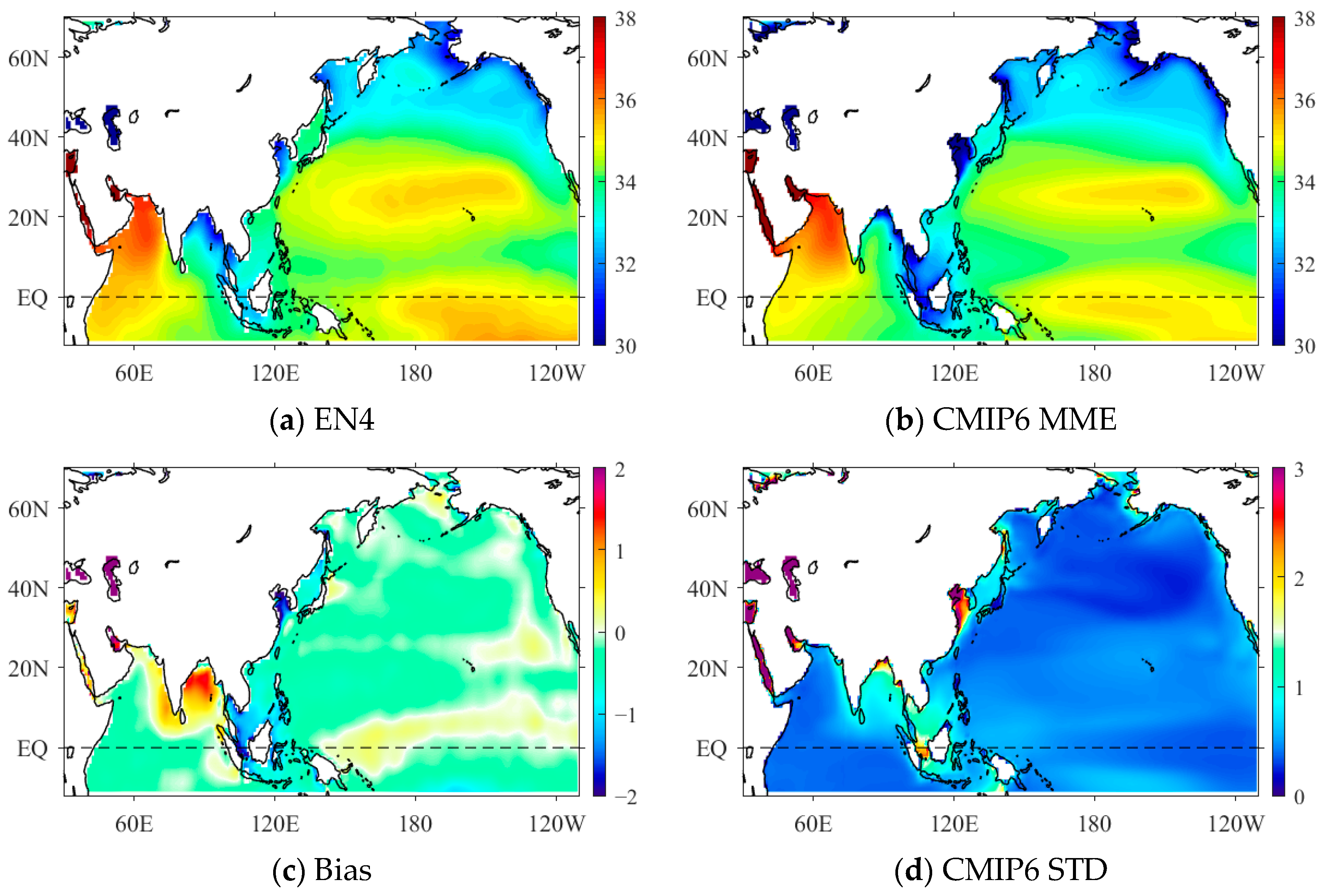
The distributions of the annual mean SSS for the observations and the multi-model ensemble mean (MME) of CMIP6 models are shown in Figure 2a,b, respectively. In the observations, the salty sea surface water is located in the Arabian Sea, with values up to 36.5 psu, while the fresh water is located in the other Asian Marginal Seas (AMSs), particularly in the Northeastern Bering Sea, the west coast of the Sea of Okhotsk, the Northern East China Seas, and the Northeastern Bay of Bengal, with typical values less than 31.5 psu (Figure 2a). The pattern of SSS distribution for CMIP6 MME is generally similar to the observations (Figure 2b). The higher salinity in the Arabian Sea is attributed to strong evaporation and the transport of saltier waters from the Red Sea, while the lower salinity in the Bay of Bengal is linked to higher precipitation and strong river runoff in this region.
Figure 2c displays the differences of the AMSs’ SSS between the CMIP6 MME and the observations. Compared to the observations, the largest negative biases are found in the Northern East China Seas, the Southern South China Sea, and the Indonesian Seas, with the bias exceeding −1.5 psu. The largest positive biases occur in the Eastern Arabian Sea and the Bay of Bengal, with values up to 1.3 psu (Figure 2c). The SSS is also underestimated in the Japan/East Sea and the South China Sea and overestimated in the Northern Bering Sea, with relatively smaller biases of approximately −0.6 and 0.2 psu, respectively (Figure 2c). The spread of models is very large in the Northern East China Seas, the north coast of the Bay of Bengal, and the Indonesian Seas in CMIP6 models, with values up to 3 (Figure 2d). In comparison to the open ocean, the simulated SSS shows relatively large differences between CMIP6 models in the coastal regions, which may be related to the poor representation of river runoff in the models.
Figure 3 shows the biases of simulated SSS in the Asian Marginal Seas in the CMIP6 models. The Bay of Bengal exhibits consistently large positive biases of approximately 1.5 psu in most CMIP6 models, which is roughly 4.6% of the observations (Figure 3). However, 10 of 41 CMIP6 models, including BCC- and CMCC-series models, FIO-ESM-2-0, ICON-ESM-LR, SAM0-UNICON, and TaiESM1, have negative biases of approximately −0.5 psu in the Bay of Bengal (Figure 3). In contrast, most CMIP6 models show fresher sea surface water in the Japan/East Sea (36 of 41), East China Seas (36 of 41), South China Sea (37 of 41), and the Indonesian Seas (38 of 41), with negative biases up to −1.9 (ACCESS-CM2), −4.3 (ACCESS-ESM1-5), −3.2 (IPSL-CM5A2-INCA), and −2.3 psu (IPSL-CM5A2-INCA), which roughly corresponds to 5.6%, 13.1%, 9.6%, and 6.8% of the observation, respectively (Figure 3). In the regions with negative SSS biases, the ACCESS-, CESM2-, CMCC-, GFDL-, and MPI-series models; FIO-ESM-2-0; and TaiEMS1 have a significantly lower simulated SSS, with biases exceeding −1.2 psu (Figure 3). In the Arabian Sea, the CMIP6 models show contradictory results in SSS simulation, with positive/negative bias in 23/18 of the models. Among all CMIP6 models, it can be found that FGOALS-g3 and MRI-ESM2-0 tend to produce systematically large SSS values in each part of the Asian Marginal Sea, with positive biases of 0.2–2.2 psu and 0.3–1.7 psu, respectively (Figure 3).
The Taylor diagram in Figure 4 displays the simulated SSS in the Asian Marginal Seas of the CMIP6 models. The observed SSS is indicated by the blue pentagram, which is located at the point with r = 1, σ = 1, and E′ = 0. A simulation point that is closer to the observation point indicates better agreement with the observations. The CMIP6 models show good agreement with the observations in the Bering Sea, Japan/East Sea, and the East China Seas, as indicated by high spatial correlations (r > 0.8 in most models) (Figure 4A,C,D). However, there are negative correlations between models and observations in the Bering Sea (GISS-E2-2-H), Japan/East Sea (FGOALS-f3-L), and the East China Seas (FGOALS-f3-L), with correlation coefficients of −0.16, −0.05, and −0.9, respectively (Figure 4A,C,D). The South China Sea exhibits the “worst” simulation, with widely dispersed correlation (0.2 < r < 0.95), spatial standard deviation (0.5 < σ < 4), and largest centered RMS error (up to 3) (Figure 4F). The Philippine Sea has the “best” simulation, with high spatial correlations (r > 0.8 in most models), moderate spatial standard deviation (0.7 < σ < 1.7), and E′ < 1 in most models (Figure 4E). The Arabian Sea also shows high spatial correlations (r > 0.75 in most models), which are above the 99% significance level, with moderate spatial standard deviation (0.5 < σ < 2) and E′ < 1.5 (Figure 4I). However, the Sea of Okhotsk, Indonesian Seas, and the Bay of Bengal have dispersed simulation points, indicating cross-model dispersion of SSS simulation in these regions among all CMIP6 models (Figure 4B,G,H).
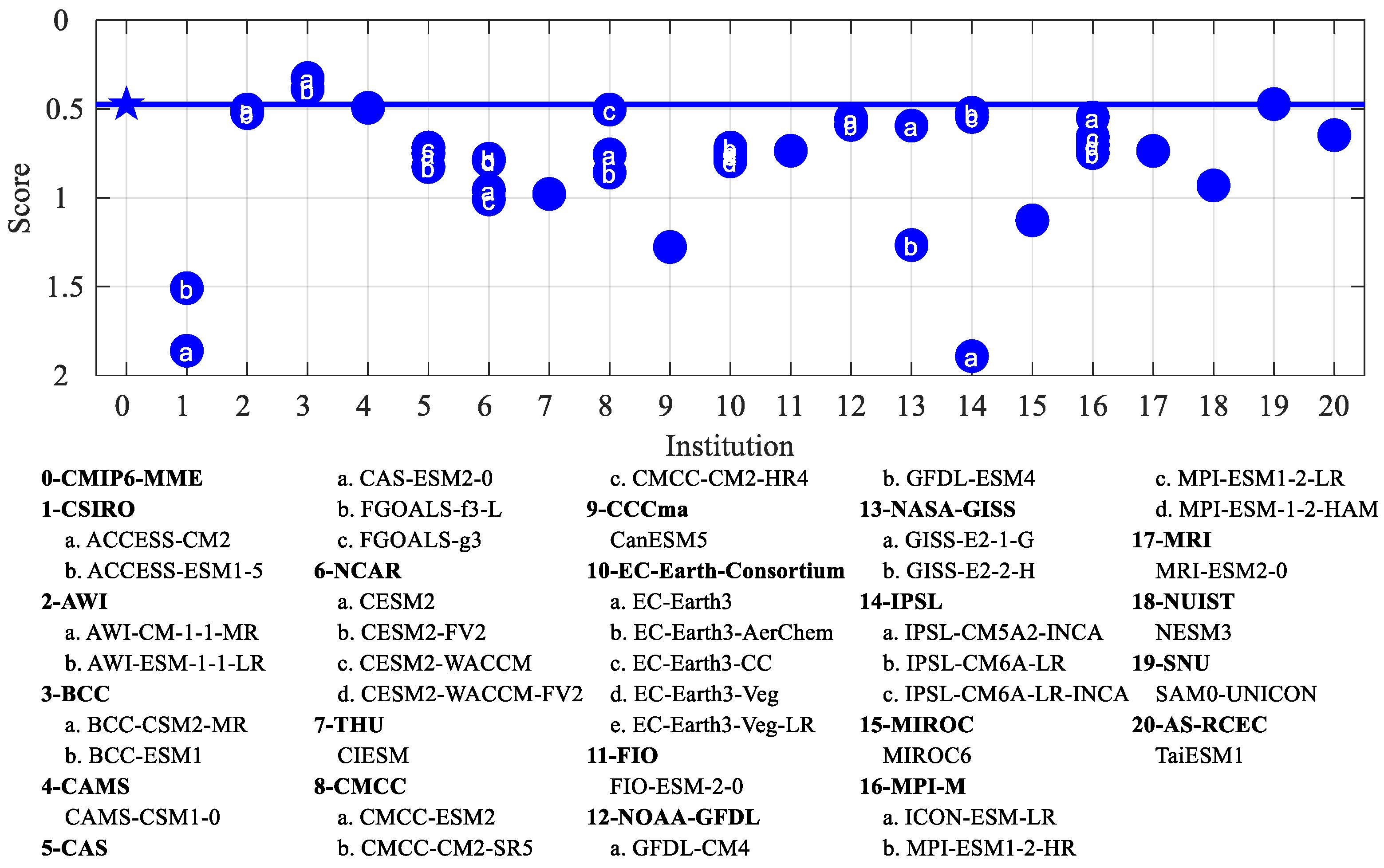
The TD scores for the AMSs’ SSS, with smaller values indicating better simulation skills, are displayed in Figure 5. The CMIP6 MMEs show better results than most CMIP6 models by averaging the errors/biases, with scores of 0.47, ranking at fourth place (Figure 5). The BCC-series models, which include BCC-CSM2-MR and BCC-ESM1, obtained the “best” AMSs’ SSS simulation, with TD scores of 0.33 and 0.39, respectively, ranking at first and second place (Figure 5). Following them is the SAM0-UNICON, which obtained TD scores of 0.47, ranking at third place, with a slightly better SSS simulation than CMIP6 MME (Figure 5). The IPSL-CM5A-INCA ranks last, with TD scores of 1.89, preceded by the ACCESS-CM2 and ACCESS-ESM1-5, with TD scores of 1.86 and 1.51, respectively, ranking second and third to last (Figure 5).
3.2. Seasonal Variation of the Spatial Mean Salinity
The salinity anomalies of the Asian Marginal Seas and the global ocean in both observations and CMIP6 models are shown in Figure 6. The salinity in the Indonesian Seas and the Arabian Sea shows a pattern where the sea surface water is fresher in the first half of the year and becomes saltier in the second half of the year, whereas the opposite is true in other Asian Marginal Seas (Figure 6). In general, the CMIP6 models reproduce the seasonal variation patterns observed in the AMSs, except for the Sea of Okhotsk, the Bay of Bengal, and the Arabian Sea (Figure 6). In the Sea of Okhotsk, the observed SSS transitions from positive anomalies in January to June and negative anomalies in July to December, while in the CMIP6 models, it changes from positive anomalies in November to May and negative anomalies in May to November, with a value of 0.7 (Figure 6B). Additionally, the EN4 dataset indicates a positive peak in May (0.3 psu) and a negative peak in September (−0.3 psu), while the CMIP6 MME shows a positive peak in March (0.7 psu) and negative peaks in July and August (−0.7 psu) in the Sea of Okhotsk (Figure 6B). In the Bay of Bengal and the Arabian Sea, there are some individual models that show different phase changes than the observations, despite the general consistency between CMIP6 MME and observations. For example, ACCESS-, BCC-, CMCC-, EC-Earth3-, and IPSL-series models in the Bay of Bengal and CAS-ESM2-0, MIROC6, NESM3, and MPI-series models in the Arabian Sea show large differences between CMIP6 models (Figure 6H,I). In the Bering Sea, the models tend to show larger SSS amplitudes than those observed (from 0.3 to −0.25 psu for the CMIP6 MME, and from 0.2 to −0.2 psu in observations; Figure 6A). However, in other Asian marginal seas, the seasonal variations of SSS are well reproduced by the CMIP6 models compared to the observations (Figure 6C–G).
The East China Seas have the largest observed magnitude (the difference between the maximum and minimum of the seasonal change) of the seasonal variation for SSS, with values of 1.2 psu, while the Philippine Sea has the smallest magnitude, with values of 0.22 psu (Figure 6D,E). In the Bering Sea and the Sea of Okhotsk, the models show a larger magnitude of variations than the observations (0.37 and 0.71 psu, respectively), with values of 0.57 and 1.35 psu for the CMIP6 MME, respectively (Figure 6A,B). By contrast, the models show a smaller magnitude of variations than the observations in the Arabian Sea, with values of 0.18 and 0.3 psu for the CMIP6 MME and the observations, respectively. Based on the global average, the magnitude of the seasonal variations for SSS is larger in the models (0.27 psu for the CMIP6 MME) than in the observations (0.2 psu) (Figure 6J). Additionally, the observed magnitude of SSS seasonal variation in the AMSs is significantly higher than the global average, with values ranging from 0.22–1.19 psu (Figure 6).
3.3. Projected SSS Trend under Different Emission Scenarios
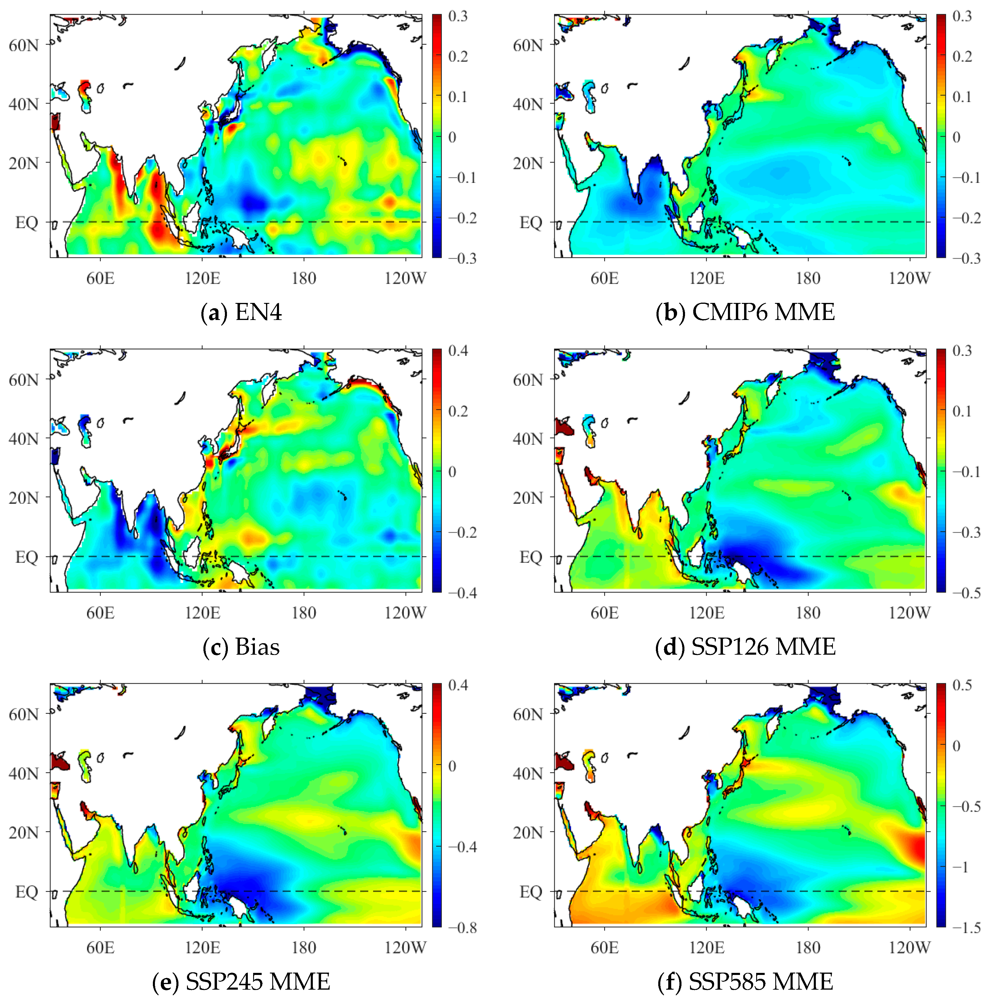
Based on EN4 observations, the largest positive trends in SSS are observed in the Eastern Arabian Sea and the Eastern Bay of Bengal. In contrast, the largest negative trends are observed in the Southern Japan/East Sea, East China Sea, and the northeast coast of the Bering Sea, with maximum values exceeding 0.25 psu/century (Figure 7a). The Bering Sea and the Sea of Okhotsk have slightly saltier sea surface water, while the South China Sea and the Indonesian Seas have fresher water, with typical values of approximately 0.08 and −0.12 psu/century, respectively (Figure 7a). The historical simulation results show positive trend of SSS occurring in the Western Sea of Okhotsk, the Western East China Sea, and the Southern South China Sea, with values less than 0.1 psu/century (Figure 7b). The simulated sea surface water is significantly fresher in the Southeastern Arabian Sea and the Western Bay of Bengal, with values of approximately −0.18 psu/century (Figure 7b). However, the distribution characteristics of the SSS trend simulated by the CMIP6 models differ significantly from those observed (Figure 7a,b). The CMIP6 models overestimate the simulated SSS trends in the Northern Japan/East Sea, Yellow Sea, South China Sea, and the Indonesian Seas, with biases of 0.07–0.2 psu/century. On the other hand, the models underestimate the trends in the Eastern Arabian Sea and the Bay of Bengal, with biases of −0.3 psu/century (Figure 7c).
In addition to historical SSS trends in the AMSs, it is critical to forecast how the SSS will change in the future. Figure 7d–f illustrate the projected spatial patterns of AMSs’ SSS trends in the future period (2015–2100) under three different scenarios: SSP126, SSP245, and SSP585. The results suggest that the SSS in the east coast of the Arabian Sea and the Central Bay of Bengal will increase in the future under the SSP126 scenario, with positive trends less than 0.25 psu/century. However, in other AMS regions, the SSS is expected to decrease, with trends ranging from −0.18 to −0.25 psu/century (Figure 7d). The SSP245 and SSP585 scenarios show negative trends in the AMSs as a whole, with values of approximately −0.25 and −0.45 psu/century, respectively (Figure 7e,f). Notably, there are significantly negative trends exceeding −0.5, −0.8, and −1.5 psu/century in the Bering Strait under the SSP126, SSP245, and SSP585 scenarios, respectively (Figure 7d–f), which may be linked to the melting of sea ice.
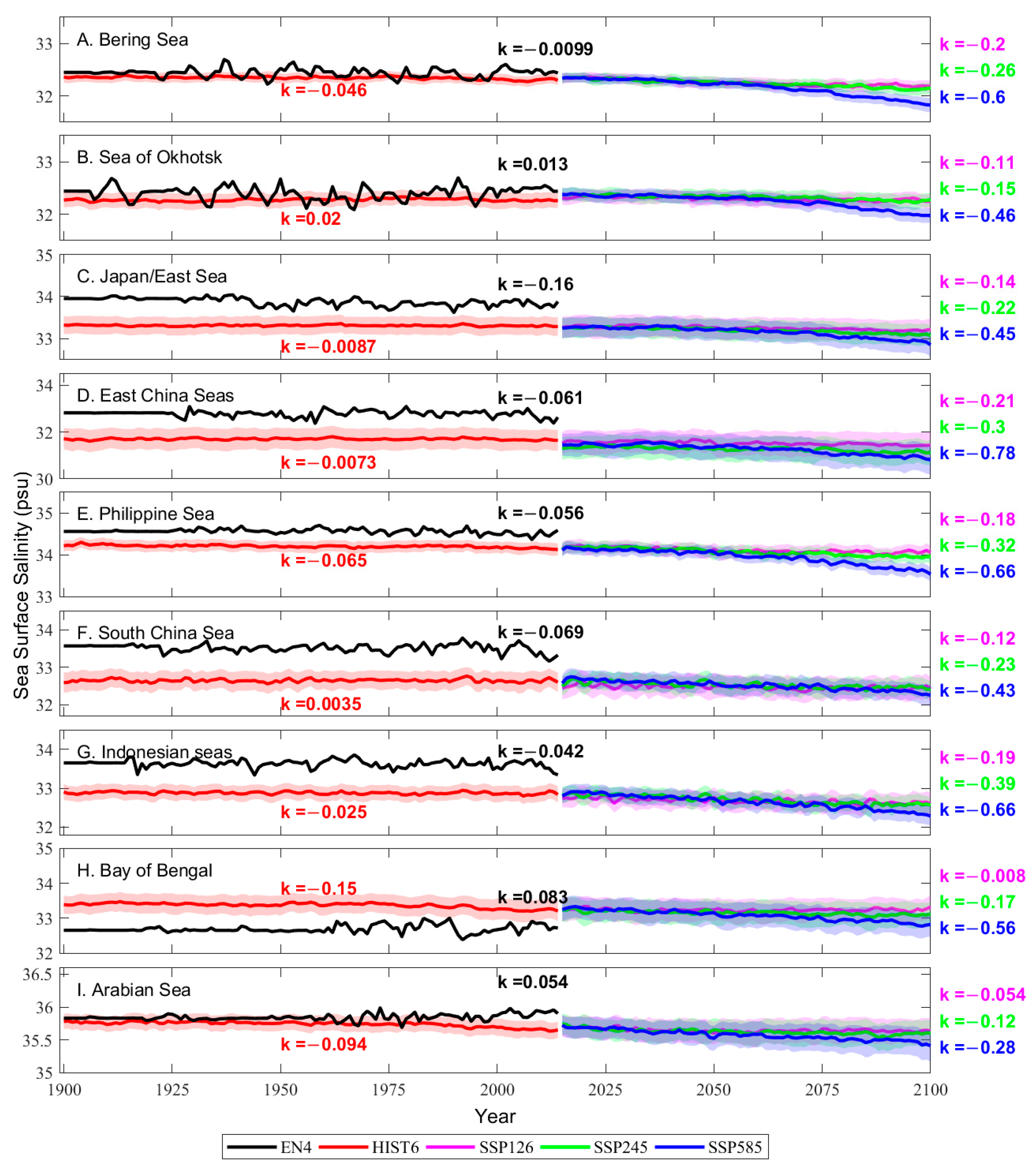
Figure 8 illustrates the spatial mean time series of SSS changes in both the observations and simulations from the CMIP6 models. The historical simulations of SSS in the Bering Sea, the Sea of Okhotsk, and the Arabian Sea exhibit smaller biases compared to the observations, while larger biases are found in the other AMS regions (Figure 8). In the historical period (1900–2014), the interannual change in SSS trends simulated by the CMIP6 models is not obvious compared with the observation. However, the historical simulations of the CMIP6 models have revealed a significant increase in negative SSS trends since 1975. For instance, the Bay of Bengal shows a spatial mean SSS trend of −0.47 psu/century in the present-day period (1976–2014), which is around 40 times larger than the past-day (1900–1975) trend of −0.012 psu/century in the CMIP6 models (Figure 8H). Similarly, in the Bering Sea and the Arabian Sea, the spatial-averaged SSS trends in the present-day period are −0.18 and −0.3 psu/century, respectively, which are about 10 times larger than the past-day trends of −0.016 and −0.041 psu/century in the CMIP6 models (Figure 8A,I). Conversely, the Indonesian Seas demonstrate an opposite trend, with SSS trends of −0.024 psu/century in the past-day period and −0.011 psu/century in the present-day period (Figure 8G). In other regions of the AMSs, the present-day SSS trends are 2–5 times larger than the past-day trends (Figure 8B–F).
In the future period (2015–2100), the projected changes in SSS by CMIP6 models are expected to occur relatively slowly in the first half of the 21st century but rapidly in the second half (Figure 8). The marginal seas are expected to exhibit negative SSS trends under different future scenarios, with a particularly obvious downward trend under the SSP585 scenario (Figure 8). In the AMSs, except for the Bay of Bengal and the Arabian Sea, the SSS trends under the SSP585 scenario were projected to be approximately three times larger than those under the SSP126 scenario (Figure 8A–G). Furthermore, in the last decade of the 21st century, the Japan/East Sea, the Philippine Sea, the South China Sea, the Indonesian Seas, and the Bay of Bengal show positive SSS trends under the SSP126 scenario, with typical values ranging from 0.13 to 0.43 psu/century.
Based on the observations, positive SSS values are found in the Sea of Okhotsk (0.013 psu/century), the Bay of Bengal (0.083 psu/century), and the Arabian Sea (0.054 psu/century) among the Asian marginal seas. The Bay of Bengal shows the largest positive SSS trend, which is about 1.8 times the global average (0.046 psu/century) (Figure 9). On the other hand, the Japan/East Sea exhibits a significant negative trend in observed SSS, which is about −0.16 psu/century (Figure 9). The simulated sea surface water in the CMIP6 historical simulation became fresher with a negative trend of −0.79 psu/century in the global ocean, which is opposite to the observed trend (Figure 9). In the CMIP6 historical simulation, the strong SSS trend is found in the Bay of Bengal, with a value of −0.15 psu/century, which is about two times the global average (Figure 9).
In the future scenarios, the SSS trends of the global annual mean are projected to be −0.1, −0.17, −0.29 psu/century in the SSP126, SSP245 and SSP585 scenarios, respectively (Figure 9). Large SSS trends are found in the East China Seas (in SSP126 and SSP585) and the Indonesian Seas (in SSP245), with values of −0.21, −0.39, and −0.78 psu/century under SSP126, SSP245, and SSP585, respectively, which are over two times larger than the global average (Figure 9). The Arabian Sea is projected to experience a slower change of SSS in the future, with values of −0.05, −0.12, and −0.28 psu/century under SSP126, SSP245, and SSP585, respectively; the change rates are slightly smaller than the global average (Figure 9).
4. Conclusions
In this study, we assessed the performance of CMIP6 models in simulating sea surface salinity (SSS) and its seasonal variations in the Asian Marginal Seas (AMSs), as well as the historical and future trends of SSS. The results indicate that although most CMIP6 models successfully capture the spatial patterns of SSS, they tend to overestimate SSS in the Eastern Arabian Sea and the Bay of Bengal and underestimate SSS in the Northern East China Seas, the Southern South China Sea, and the Indonesian Seas. Additionally, the CMIP6 models perform the best in the Philippine Sea and worst in the South China Sea. Overall, the CMIP6 MME obtained a TD score of 0.47, ranking at the fourth place. Among individual models, BCC-CSM2-MR, BCC-ESM1, and SAM0-UNICON show a better SSS simulation performance than the CMIP6 MME, with TD scores of 0.33, 0.39, and 0.47, respectively, ranking first to third. In contrast, IPSL-CM5A-INCA and ACCESS-series models perform poorly in SSS simulation, with TD scores exceeding 1.5 and ranking last.
Next, we analyzed the seasonal variations of SSS in both the AMSs and the global ocean, using both the observations and the CMIP6 models. The results reveal that surface water is typically saltier in the first half of the year but becomes fresher in the second half of the year, with the exception of the Indonesian Seas and the Arabian Sea. In comparison with the observations, large biases of seasonal variation occur in the Sea of Okhotsk, the Bay of Bengal, and the Arabian Sea, with some CMIP6 models exhibiting phase shift or reversal. Notably, the observed magnitudes in the AMSs are significantly higher than those in the global average (0.2 psu), with typical values ranging from 0.22 psu in the Philippine Sea to 1.19 psu in the East China Seas.
Finally, we analyzed the SSS trends in the AMSs for both historical (1900–2014) and future scenarios (2015–2100), using CMIP6 models. During the history period, the observed SSS showed a significant positive trend in the Eastern Arabian Sea and the Eastern Bay of Bengal. On the other hand, the Southern Japan/East Sea, East China Sea, and the northeast coast of the Bering Sea showed a largest negative trend. However, the simulated SSS shows negative trends in the Arabian Sea and the Bay of Bengal, with typical values of approximately −0.18 psu/century. In the future period, the SSS freshening trends are projected to be relatively faster in the second half of the 21st century than in the first half. The CMIP6 models show freshening trends of 0.05–0.21, 0.12–0.39, and 0.28–0.78 psu/century for the SSP126, SSP245, and SSP585, respectively. The most rapid SSS freshening trends are observed in the East China Seas, and the Indonesian Seas, which are over two times greater than the global mean. In contrast, the SSS freshening trends in the Arabian Sea are relatively slow, with typical values slightly smaller than the global mean trend.
Sea surface salinity is a crucial indicator of the ocean hydrological cycle and has a significant impact on the properties and energy of tropical instability waves (TIWs) [39]. Additionally, it is highly responsive to tropical cyclones [40]. Therefore, it is essential to accurately simulate SSS. Furthermore, the projected SSS can be valuable in assessing climate change and making ecosystem-based management decisions in marginal seas [41]. In the future, it can be expected that the surface water will become fresher, which will increase surface stratification and hinder vertical mixing. This will have a direct influence on species at all levels.
Author Contributions
Conceptualization, T.X. and S.J.; methodology, S.J.; software, S.J.; validation, T.X. and H.P.; formal analysis, S.J.; investigation, S.J.; resources, T.X.; data curation, S.J.; writing—original draft preparation, S.J.; writing—review and editing, S.J., T.X. and H.P.; visualization, S.J.; supervision, T.X.; project administration, T.X.; funding acquisition, T.X. All authors have read and agreed to the published version of the manuscript.
Funding
This research was jointly funded by the Laoshan Laboratory (Contact No. LSKJ202202700).
Institutional Review Board Statement
Not applicable.
Informed Consent Statement
Not applicable.
Data Availability Statement
The observed SSS data are available at https://www.metoffice.gov.uk/hadobs/en4/download-en4-2-1.html accessed on 12 February 2023. The SSS data from CMIP6 models are available at https://esgf-node.llnl.gov/projects/cmip6/ accessed on 12 February 2023.
Acknowledgments
The authors are really grateful to the EN4 data provider.
Conflicts of Interest
The authors declare no conflict of interest.
References
- Schmitt, R. Salinity and the Global Water Cycle. Oceanography 2008, 21, 12. [Google Scholar] [CrossRef]
- Helm, K.P.; Bindoff, N.L.; Church, J.A. Changes in the global hydrological-cycle inferred from ocean salinity. Geophys. Res. Lett. 2010, 37, L18701. [Google Scholar] [CrossRef]
- Durack, P.J.; Wijffels, S.E. Fifty-year trends in global ocean salinities and their relationship to broad-scale warming. J. Clim. 2010, 23, 4342–4362. [Google Scholar] [CrossRef]
- Skliris, N.; Marsh, R.; Josey, S.A.; Good, S.A.; Liu, C.; Allan, R.P. Salinity changes in the World Ocean since 1950 in relation to changing surface freshwater fluxes. Clim. Dyn. 2014, 43, 709–736. [Google Scholar] [CrossRef]
- Delcroix, T. Observed surface oceanic and atmospheric variability in the tropical Pacific at seasonal and ENSO timescales: A tentative overview. J. Geophys. Res. Ocean. 1998, 103, 18611–18633. [Google Scholar] [CrossRef]
- Ballabrera-poy, J.; Murtugudde, R.; Busalacchi, A.J. On the potential impact of sea surface salinity observations on ENSO predictions. J. Geophys. Res. 2002, 107, 8007. [Google Scholar] [CrossRef]
- Maes, C.; Picaut, J.; Belamari, S. Salinity barrier layer and onset of El Nino in a Pacific coupled model. Geophys. Res. Lett. 2002, 29, 59. [Google Scholar] [CrossRef]
- Zhu, J.; Huang, B.; Zhang, R.-H.; Hu, Z.-Z.; Kumar, A.; Balmaseda, M.A.; Marx, L.; Kinter, J.L., III. Salinity anomaly as a trigger for ENSO events. Sci. Rep. 2014, 4, 6821. [Google Scholar] [CrossRef]
- Qu, T.; Yu, J.-Y. ENSO indices from sea surface salinity observed by Aquarius and Argo. J. Oceanogr. 2014, 70, 367–375. [Google Scholar] [CrossRef]
- Reverdin, G.; Kestenare, E.; Frankignoul, C.; Delcroix, T. Surface salinity in the Atlantic Ocean (30 S–50 N). Prog. Oceanogr. 2007, 73, 311–340. [Google Scholar] [CrossRef]
- Friedman, A.R.; Reverdin, G.; Khodri, M.; Gastineau, G. A new record of Atlantic sea surface salinity from 1896 to 2013 reveals the signatures of climate variability and long-term trends. Geophys. Res. Lett. 2017, 44, 1866–1876. [Google Scholar] [CrossRef]
- Delcroix, T.; Henin, C.; Porte, V.; Arkin, P. Precipitation and sea-surface salinity in the tropical Pacific Ocean. Deep. Sea Res. Part I Oceanogr. Res. Pap. 1996, 43, 1123–1141. [Google Scholar] [CrossRef]
- Wang, G.; Cheng, L.; Boyer, T.P.; Li, C. Halosteric Sea Level Changes during the Argo Era. Water 2017, 9, 484. [Google Scholar] [CrossRef]
- Lee, T.; Lagerloef, G.; Gierach, M.M.; Kao, H.Y.; Yueh, S.; Dohan, K. Aquarius reveals salinity structure of tropical instability waves. Geophys. Res. Lett. 2012, 39, L12610. [Google Scholar] [CrossRef]
- Yin, X.; Boutin, J.; Reverdin, G.; Lee, T.; Arnault, S.; Martin, N. SMOS Sea Surface Salinity signals of tropical instability waves. J. Geophys. Res. Ocean. 2014, 119, 7811–7826. [Google Scholar] [CrossRef]
- Menezes, V.V.; Vianna, M.L.; Phillips, H.E. Aquarius sea surface salinity in the South Indian Ocean: Revealing annual-period planetary waves. J. Geophys. Res. Ocean. 2014, 119, 3883–3908. [Google Scholar] [CrossRef]
- Roemmich, D.; Morris, M.; Young, W.R.; Donguy, J.R. Fresh equatorial jets. J. Phys. Oceanogr. 1994, 24, 540–558. [Google Scholar] [CrossRef]
- Lagerloef, G.; Schmitt, R.; Schanze, J.; Kao, H.-Y. The Ocean and the global water cycle. Oceanography 2010, 23, 82–93. [Google Scholar] [CrossRef]
- Delworth, T.; Manabe, S.; Stouffer, R.J. Interdecadal variations of the thermohaline circulation in a coupled oceanatmosphere model. J. Clim. 1993, 6, 1993–2011. [Google Scholar] [CrossRef]
- Delworth, T.L.; Rosati, A.; Anderson, W.; Adcroft, A.J.; Balaji, V.; Benson, R.; Dixon, K.; Griffies, S.; Lee, H.-C.; Pacanowski, R.C.; et al. Simulated climate and climate change in the GFDL CM2.5 high-resolution coupled climate model. J. Clim. 2012, 25, 2755–2781. [Google Scholar] [CrossRef]
- Danabasoglu, G.; Yeager, S.G.; Kwon, Y.-O.; Tribbia, J.J.; Phillips, A.S.; Hurrell, J.W. Variability of the Atlantic meridional overturning circulation in CCSM4. J. Clim. 2012, 25, 5153–5172. [Google Scholar] [CrossRef]
- Kwon, Y.O.; Frankignoul, C. Stochastically-driven multidecadal variability of the Atlantic meridional overturning circulation in CCSM3. Clim. Dyn. 2012, 38, 859–876. [Google Scholar] [CrossRef]
- Liu, W.; Fedorov, A.V.; Xie, S.P.; Hu, S.N. Climate impacts of a weakened Atlantic Meridional Overturning Circulation in a warming climate. Sci. Adv. 2020, 6, eaaz4876. [Google Scholar] [CrossRef] [PubMed]
- Zhuang, T.P.; Jin, H.Y.; Gu, F.; Zhang, Y.; Bai, Y.; Ji, Z.; Lu, Y.; Chen, J. Composition of algal pigments in surface freshen layer after ice melt in the central Arctic. Acta Oceanol. Sin. 2017, 36, 122–130. [Google Scholar] [CrossRef]
- Liu, Y.; Cheng, L.; Pan, Y.; Tan, Z.; Abraham, J.; Zhang, B.; Zhu, J.; Song, J. How Well Do CMIP6 and CMIP5 Models Simulate the Climatological Seasonal Variations in Ocean Salinity? Adv. Atmos. Sci. 2022, 39, 1650–1672. [Google Scholar] [CrossRef]
- Fathrio, I.; Manda, A.; Iizuka, S.; Kodama, Y.M.; Ishida, S. Evaluation of CMIP5 models on sea surface salinity in the Indian Ocean. IOP Conf. Ser. Earth Environ. Sci. 2017, 54, 012039. [Google Scholar] [CrossRef]
- Meehl, G.A.; Boer, G.J.; Covey, C.; Latif, M.; Stouffer, R.J. Intercomparison makes for a better climate model. Eos Trans. Am. Geophys. Union 1997, 78, 445–451. [Google Scholar] [CrossRef]
- Meehl, G.A.; Boer, G.J.; Covey, C.; Latif, M.; Stouffer, R.J. The Coupled Model Intercomparison Project (CMIP). Bull. Am. Meteorol. Soc. 2000, 81, 313–318. [Google Scholar] [CrossRef]
- Meehl, G.A.; Covey, C.; Delworth, T.; Latif, M.; McAvaney, B.; Mitchell, J.F.B.; Stouffer, R.J.; Taylor, K.E. The WCRP CMIP3 multimodel dataset: A new era in climate change research. Bull. Am. Meteorol. Soc. 2007, 88, 1383–1394. [Google Scholar] [CrossRef]
- Taylor, K.E.; Stouffer, R.J.; Meehl, G.A. An overview of CMIP5 and the experiment design. Bull. Am. Meteorol. Soc. 2012, 93, 485–498. [Google Scholar] [CrossRef]
- Eyring, V.; Bony, S.; Meehl, G.A.; Senior, C.A.; Stevens, B.; Stouffer, R.J.; Taylor, K.E. Overview of the Coupled Model Inter comparison Project Phase 6 (CMIP6) experimental design and organization. Geosci. Model Dev. 2016, 9, 1937–1958. [Google Scholar] [CrossRef]
- Intergovernmental Panel on Climate Change. Evaluation of Climate Models. In Climate Change 2013: The Physical Science Basis. Contribution of Working Group I to the Fifth Assessment Report of the Intergovernmental Panel on Climate Change; Stocker, T.F., Qin, D., Plattner, G.-K., Tignor, M., Allen, S., Boschung, J., Nauels, A., Xia, Y., Bex, V., Midgley, P., Eds.; Cambridge University Press: Cambridge, UK, 2013; Volume 9, pp. 741–886. [Google Scholar]
- Eyring, V.; Gillett, N.P. Human influence on the climate system. In Climate Change 2021: The Physical Science Basis. Contribution of Working Group I to the Sixth Assessment Report of the Intergovernmental Panel on Climate Change; Masson-Delmotte, V., Zhai, P., Pirani, A., Connors, S., Péan, C., Berger, S., Caud, N., Chen, Y., Goldfarb, L., Gomis, M., et al., Eds.; Cambridge University Press: Cambridge, UK, 2021; Volume 3, pp. 478–481. [Google Scholar]
- Lin, J.L. The double-ITCZ problem in IPCC AR4 Coupled GCMs: Ocean-atmosphere feedback analysis. J. Clim. 2007, 20, 4497–4525. [Google Scholar] [CrossRef]
- Zhang, R.H.; Busalacchi, A.J. Freshwater flux (FWF) induced oceanic feedback in a hybrid coupled model of the tropical Pacific. J. Clim. 2009, 22, 853–879. [Google Scholar] [CrossRef]
- Zhi, H.; Huang, Y.; Lin, P.; Shi, S.; Dong, M. Interannual variability of the sea surface salinity and its related freshwater flux in the tropical Pacific: A comparison of CMIP5 and CMIP6. Atmos. Ocean. Sci. Lett. 2022, 15, 100190. [Google Scholar] [CrossRef]
- Good, S.A.; Martin, M.J.; Rayner, N.A. EN4: Quality controlled ocean temperature and salinity profiles and monthly objectively analyses with uncertainty estimates. J. Geophys. Res. Ocean. 2013, 118, 6704–6716. [Google Scholar] [CrossRef]
- Taylor, K.E. Summarizing multiple aspects of model performance in a single diagram. J. Geophys. Res. Atmos. 2001, 106, 7183–7192. [Google Scholar] [CrossRef]
- Reul, N.; Chapron, B.; Grodsky, S.A.; Guimbard, S.; Kudryavtsev, V.; Foltz, G.R.; Balaguru, K. Satellite observations of the sea surface salinity response to tropical cyclones. Geophys. Res. Lett. 2021, 48, e2020GL091478. [Google Scholar] [CrossRef]
- Olivier, L.; Reverdin, G.; Hasson, A.; Boutin, J. Tropical instability waves in the Atlantic ocean: Investigating the relative role of sea surface salinity and temperature from 2010 to 2018. J. Geophys. Res. Ocean. 2020, 125, e2020JC016641. [Google Scholar] [CrossRef]
- Walker, S.; Mozaria-Luna, H.N.; Kaplan, I.; Petatán-Ramírez, D. Future temperature and salinity in Puget Sound, Washington State, under CMIP6 climate change scenarios. J. Water Clim. Chang. 2022, 13, 124255. [Google Scholar] [CrossRef]
Figure 1.
Study regions of the Asian Marginal Seas (AMSs), with a background color map representing the distribution of the climatological annual mean sea surface salinity (unit: psu). The study regions are indicated by boxes, as follows: A. Bering Sea; B. Sea of Okhotsk; C. Japan/East Sea; D. East China Seas (including the East China Sea, the Yellow Sea, and the Bohai Sea, ECSs); E. Philippine Sea; F. South China Sea (SCS); G. Indonesian Seas; H. Bay of Bengal; and I. Arabian Sea.

Figure 2.
Observed and simulated annual mean sea surface salinity (SSS; unit: psu). (a) EN4; (b) multi-model ensemble mean (MME) of the CMIP6 models; (c) biases between the CMIP6 MME and EN4; (d) cross-model standard deviation of the simulated SSS in the CMIP6 models.
Figure 2.
Observed and simulated annual mean sea surface salinity (SSS; unit: psu). (a) EN4; (b) multi-model ensemble mean (MME) of the CMIP6 models; (c) biases between the CMIP6 MME and EN4; (d) cross-model standard deviation of the simulated SSS in the CMIP6 models.

Figure 3.
Model biases of area-averaged sea surface salinity in CMIP6 models compared with EN4 observations (unit: psu). The alphabetical order of A–I in the x-axis represents different Asian Marginal Seas that are marked by boxes in Figure 1. A. Bering Sea; B. Sea of Okhotsk; C. Japan/East Sea; D. East China Seas (including the East China Sea, the Yellow Sea, and the Bohai Sea, ECSs); E. Philippine Sea; F. South China Sea (SCS); G. Indonesian Seas; H. Bay of Bengal; and I. Arabian Sea.

Figure 4.
Taylor Diagram of simulated annual mean sea surface salinity (SSS) in different regions of the Asian Marginal Seas (AMSs) in the CMIP6 models. ((A) Bering Sea, (B) Sea of Okhotsk, (C) Japan/East Sea (JES), (D) East China Seas (ECSs), (E) Philippine Sea, (F) South China Sea (SCS), (G) Indonesian Seas, (H) Bay of Bengal, and (I) Arabian Sea.) The black solid contours indicate the normalized spatial standard deviation (σm/σo) with respect to that of EN4 (σo). The dashed blue contours and dashed black lines indicate the centered root-mean-square bias (E′) and spatial correlation coefficient (r) of annual mean SSS between models and EN4, respectively. The EN4 is defined as the reference point (blue pentagram), with normalized spatial standard deviation (σo/σo), E′, and R equal to 1, 0, and 1, respectively. The black pentagrams donate the CMIP6 multi-model ensemble means (MMEs). The σm, σo, E′, and R are defined in Section 2.2.

Figure 5.
Taylor Diagram Score of the simulated sea surface salinity (SSS) in the Asia Marginal Seas (AMSs). Blue pentagrams indicate the CMIP6 multi-model ensemble means (MMEs), with scores of 0.47. The sequence numbers from 1 to 20 are affiliated with the institutions listed in Table 1.
Figure 5.
Taylor Diagram Score of the simulated sea surface salinity (SSS) in the Asia Marginal Seas (AMSs). Blue pentagrams indicate the CMIP6 multi-model ensemble means (MMEs), with scores of 0.47. The sequence numbers from 1 to 20 are affiliated with the institutions listed in Table 1.

Figure 6.
Spatial mean seasonal variation of the sea surface salinity (SSS) of each part of the Asian Marginal Seas (A–I) and global mean SSS (J) in the observations and the CMIP6 models. The salinity anomalies are relative to the annual average. The red and black solid contours indicate the observations and CMIP6 multi-model ensemble means, respectively.

Figure 7.
Linear trends of the sea surface salinity (SSS) for the historical period (1900–2014) and the future period (2015–2100). (a) EN4; (b) multi-model ensemble mean (MME) of the CMIP6 historical simulation; (c) biases between the CMIP6 MME and EN4; (d) SSP126, (e) SSP245, and (f) SSP585 are the multi-model ensemble means of the SSS trend for the future scenario simulations under the Shared Socio-Economic Pathway (SSP) in CMIP6 models (unit: psu/century).

Figure 8.
Spatial mean time series of sea surface salinity (SSS; unit: psu) from observation (black), multi-model ensemble means (MME) of the CMIP6 historical simulation (red), and MME of the simulations under SSP126 (pink), SSP245 (green), and SSP585 (blue), with the uncertainty between the models (shaded) for the Asian Marginal Seas (AMSs) in January. The “k” means the SST trend for historical (1900–2014) or future (2015–2100) period (unit: psu/century), and different colors of “k” correspond to the colorful line.

Figure 9.
Trends of spatial mean sea surface salinity (SSS) in the global and each Asian Marginal Sea (unit: psu/century). The alphabetical order of A–I in the x-axis represents different Asian Marginal Seas that are marked by boxes in Figure 1. A. Bering Sea; B. Sea of Okhotsk; C. Japan/East Sea; D. East China Seas (including the East China Sea, the Yellow Sea, and the Bohai Sea, ECSs); E. the Philippine Sea; F. the South China Sea (SCS); G. Indonesian Seas; H. Bay of Bengal; and I. Arabian Sea.


Table 1.
Details of models used in CMIP6 analysis of Asia Marginal Seas (AMSs).
| No. | Institute (Country) | Model Name | Resolution (lon × lat) | HIST6 | SSP126 | SSP245 | SSP585 |
|---|---|---|---|---|---|---|---|
| 1 | CSIRO (Australia) | ACCESS-CM2 | 360 × 300 | √ | √ | √ | √ |
| ACCESS-ESM1-5 | 360 × 300 | √ | √ | √ | √ | ||
| 2 | AWI (Germany) | AWI-CM-1-1-MR | 830,305 × 1 | √ | √ | √ | √ |
| AWI-ESM-1-1-LR | 126,859 × 1 | √ | × | × | × | ||
| 3 | BCC (China) | BCC-CSM2-MR | 360 × 232 | √ | √ | √ | √ |
| BCC-ESM1 | 360 × 232 | √ | × | × | × | ||
| 4 | CAMS (China) | CAMS-CSM1-0 | 360 × 200 | √ | √ | √ | √ |
| 5 | CAS (China) | CAS-ESM2-0 | 360 × 196 | √ | √ | √ | √ |
| FGOALS-f3-L | 360 × 218 | √ | √ | × | √ | ||
| FGOALS-g3 | 360 × 218 | √ | √ | √ | √ | ||
| 6 | NCAR (USA) | CESM2 | 320 × 384 | √ | × | × | × |
| CESM2-FV2 | 320 × 384 | √ | × | × | × | ||
| CESM2-WACCM | 320 × 384 | √ | √ | √ | √ | ||
| CESM2-WACCM-FV2 | 320 × 384 | √ | × | × | × | ||
| 7 | YHU (China) | CIESM | 320 × 384 | √ | √ | √ | √ |
| 8 | CMCC (Italy) | CMCC-CM2-HR4 | 1442 × 1051 | √ | × | × | × |
| CMCC-CM2-SR5 | 362 × 292 | √ | √ | √ | √ | ||
| CMCC-ESM2 | 362 × 292 | √ | √ | √ | √ | ||
| 9 | CCCma (Canada) | CanESM5 | 360 × 291 | √ | √ | √ | √ |
| 10 | EC-Earth-Consortium (Europe) | EC-Earth3 | 362 × 292 | √ | √ | √ | √ |
| EC-Earth3-AerChem | 362 × 292 | √ | × | × | × | ||
| EC-Earth3-CC | 362 × 292 | √ | × | √ | √ | ||
| EC-Earth3-Veg | 362 × 292 | √ | √ | √ | √ | ||
| EC-Earth3-Veg-LR | 362 × 292 | √ | √ | √ | √ | ||
| 11 | FIO (China) | FIO-ESM-2-0 | 320 × 384 | √ | √ | √ | √ |
| 12 | NOAA-GFDL (USA) | GFDL-CM4 | 1440 × 1080 | √ | × | √ | √ |
| GFDL-ESM4 | 720 × 576 | √ | √ | √ | √ | ||
| 13 | NASA-GISS (USA) | GISS-E2-1-G | 288 × 180 | √ | × | × | × |
| GISS-E2-2-H | 360 × 180 | √ | × | × | × | ||
| 14 | IPSL (France) | IPSL-CM5A2-INCA | 182 × 149 | √ | √ | × | × |
| IPSL-CM6A-LR | 362 × 332 | √ | √ | √ | √ | ||
| IPSL-CM6A-LR-INCA | 362 × 332 | √ | × | × | × | ||
| 15 | MIROC (Japan) | MIROC6 | 360 × 256 | √ | √ | √ | √ |
| 16 | MPI-M (Germany) | ICON-ESM-LR | 235,403 × 1 | √ | × | × | × |
| MPI-ESM-1-2-HAM | 256 × 220 | √ | × | × | × | ||
| MPI-ESM1-2-HR | 802 × 404 | √ | √ | √ | √ | ||
| MPI-ESM1-2-LR | 256 × 220 | √ | √ | √ | √ | ||
| 17 | MRI (Japan) | MRI-ESM2-0 | 360 × 363 | √ | √ | √ | √ |
| 18 | NUIST (China) | NESM3 | 362 × 292 | √ | √ | √ | √ |
| 19 | SNU (Korea) | SAM0-UNICON | 320 × 384 | √ | × | × | × |
| 20 | AS-RCEC (China) | TaiESM1 | 320 × 384 | √ | √ | √ | √ |
Note: Resolution is represented by the grid numbers of longitude × latitude. The available and unavailable outputs are marked by “√” and “×” for the historical (HIST6), the SSP126, SSP245, and SSP585, respectively.
Disclaimer/Publisher’s Note: The statements, opinions and data contained in all publications are solely those of the individual author(s) and contributor(s) and not of MDPI and/or the editor(s). MDPI and/or the editor(s) disclaim responsibility for any injury to people or property resulting from any ideas, methods, instructions or products referred to in the content. |
© 2023 by the authors. Licensee MDPI, Basel, Switzerland. This article is an open access article distributed under the terms and conditions of the Creative Commons Attribution (CC BY) license (https://creativecommons.org/licenses/by/4.0/).
Share and Cite
MDPI and ACS Style
Jin, S.; Pan, H.; Xu, T. Assessment of the Sea Surface Salinity Simulation and Projection Surrounding the Asian Waters in the CMIP6 Models. Atmosphere 2023, 14, 726. https://doi.org/10.3390/atmos14040726
AMA Style
Jin S, Pan H, Xu T. Assessment of the Sea Surface Salinity Simulation and Projection Surrounding the Asian Waters in the CMIP6 Models. Atmosphere. 2023; 14(4):726. https://doi.org/10.3390/atmos14040726
Chicago/Turabian StyleJin, Shanshan, Haidong Pan, and Tengfei Xu. 2023. "Assessment of the Sea Surface Salinity Simulation and Projection Surrounding the Asian Waters in the CMIP6 Models" Atmosphere 14, no. 4: 726. https://doi.org/10.3390/atmos14040726
Note that from the first issue of 2016, this journal uses article numbers instead of page numbers. See further details here.