
I-Solar, a Real-Time Photovoltaic Simulation Model for Accurate Estimation of Generated Power


1
Regional Development Institute, University of Castilla-La Mancha, Paseo de los Estudiantes s/n, 02006 Albacete, Spain
2
Regional Centre of Water Research, University of Castilla-La Mancha, Ctra de Las Peñas 3.2, 02071 Albacete, Spain
*
Author to whom correspondence should be addressed.
Agronomy 2021, 11(3), 485; https://doi.org/10.3390/agronomy11030485
Submission received: 27 January 2021
/
Revised: 28 February 2021
/
Accepted: 1 March 2021
/
Published: 5 March 2021
(This article belongs to the Special Issue Modernization and Optimization of Irrigation Systems)
Abstract
:Global energy consumption and costs have increased exponentially in recent years, accelerating the search for viable, profitable, and sustainable alternatives. Renewable energy is currently one of the most suitable alternatives. The high variability of meteorological conditions (irradiance, ambient temperature, and wind speed) requires the development of complex and accurate management models for the optimal performance of photovoltaic systems. The simplification of photovoltaic models can be useful in the sizing of photovoltaic systems, but not for their management in real time. To solve this problem, we developed the I-Solar model, which considers all the elements that comprise the photovoltaic system, the meteorologic conditions, and the energy demand. We have validated it on a solar pumping system, but it can be applied to any other system. The I-Solar model was compared with a simplified model and a machine learning model calibrated in a high-power and complex photovoltaic pumping system located in Albacete, Spain. The results show that the I-Solar model estimates the generated power with a relative error of 7.5%, while the relative error of machine learning models was 5.8%. However, models based on machine learning are specific to the system evaluated, while the I-Solar model can be applied to any system.
1. Introduction
One of the biggest threats facing the world population is climate change, which is primarily caused by the emission of greenhouse gases (GHG) produced by the use of fossil fuels in industrial processes. The benefits of renewable energy (REn) are clearly visible, being a prerequisite to reach socioeconomically sustainable systems, and particularly to address the challenges of climate change and the depletion of fossil fuels. These problems require active policies aiming at a rapid transition [1,2]. Thus, REn is presented as a viable and profitable alternative to the use of conventional sources of electricity [3].
Among the different sources of renewable energy, photovoltaic solar energy is in a period of high growth globally [4]. The most important factor for the establishment of this type of system is the cost [5,6]. However, the price of all components included in a photovoltaic installation has drastically decreased in recent years [7], with a drop of up to 85% in the cost of photovoltaic modules [8]. The improvement of photovoltaic modules and the search for highly efficient new materials [9] or module types [10] has led to an expansion, with high levels of investment in photovoltaic solar energy as an alternative to conventional energy sources. Some studies analyzed the competition for land between photovoltaic energy producers and farmers, which can be balanced in what is called agrivoltaics [11]. Although agrivoltaics can open up an additional revenue stream, there is a high concern by farmers about land affection on the long term.
The energy consumption in irrigation agriculture has exponentially increased in recent years due to the modernisation of irrigation systems, from surface irrigation to pressurised irrigation [12,13]. It is necessary to find more efficient alternatives [14], mainly in areas with high energy demand, such as irrigable areas with underground water resources, where the extraction cost can reach up to 70% of the total energy cost of irrigation [15]. One of the possible alternatives to decrease the water extraction and application costs is the integration of photovoltaic energy [3,16,17,18]. Photovoltaic pumping systems have already been established in many countries including the USA [19], India [20], Turkey [21], Spain [12,22] and Algeria [23]. However, the photovoltaic pumping systems must be managed properly to obtain quality irrigation, even in complex irrigation systems [24].
Great advances have been made in the development of methodologies to design photovoltaic pumping systems and other uses, such as the Photovoltaic Geographical Information System (PVGIS, http://re.jrc.ec.europa.eu/pvgis/). However, the optimal management of a system, once sized and installed, is a key factor in the satisfactory performance of the system, which requires the development of real-time simulation models. To efficiently manage photovoltaic pumping systems after installation, the following actions need to be taken: (1) generate simulation models of irradiance (W·m−2) on inclined surfaces, in order to estimate in an accurate manner the real-time direct, diffuse and reflected components of the irradiance; (2) generate simulation models of photovoltaic generators that represent accurately and in real-time the generated power (current and voltage in direct current (DC) and alternating current (AC)); and (3) characterize the operation of the equipment required to feed the system, such as the variable frequency drive (VFD) and cables. A successful experience was implemented in Palestine by generating a micro-grid solar photovoltaic systems for rural development and sustainable agriculture [25]. However, an improvement of the described results would be expected if a more accurate solar model was utilized, as proposed in this manuscript.
In addition, in the process of sizing the photovoltaic pumping systems, the photovoltaic generator is frequently oversized to absorb the high uncertainty in the irradiance data, and can be of up to 30% [26], among other factors. This is a practical measure to ensure the adequate performance of the system, but requires proper regulation, which is usually not well defined. In addition, it increases the complexity of the simulation owing to the necessity of including a regulation algorithm for these cases with excess power generation due to oversizing. Although important developments in photovoltaic simulation models have been realized, no analysis of the effects of the oversizing of the photovoltaic generator on the final operation of the system have been found. Thus, it is necessary for methodologies to generate robust models that allow accurate simulation of the photovoltaic power generated in real time, which is essential for adequate irrigation management.
There are many models to estimate the direct and diffuse components of global irradiance [27,28] that allow these components to be obtained from daily global irradiance values. Erbs et al. [29] developed a model to estimate the diffuse radiation fraction for hourly, daily, and monthly average global radiation. Muneer [30] and Duffie and Beckman [31] established some simplifications, known internationally, considering an isotropic distribution of diffuse irradiance. Shen et al. [32] developed, based on previous references and some modifications, a simulation model of the solar radiation using the Simulink module of Matlab® (Mathworks Inc., Massachusetts, USA). In addition, there are various applications of free software such as PVGIS that offer statistical data provided by satellites to estimate the solar radiation. The model proposed in this work for the calculation of diffuse irradiance [33] is one of the most used models to estimate the diffuse irradiance on an inclined surface [34], offering accurate results [35]. Thus, it is necessary to develop simulation models that work with irradiance values (W·m−2), which ensure adequate management in real-time once the system has been sized.
There are many models to estimate the generated power in photovoltaic modules. These include: (1) based on the calculation of the fill factor [36]; (2) by determining the short circuit current and open circuit voltage variation at a certain temperature of operation [37]; (3) determining the current and voltage at the maximum power point (MPP) [38]; (4) a simulation procedure for the prediction of monthly energy provided by photovoltaic systems based on daily profiles of irradiance and temperature [39]; (5) methods to increase the output efficiency of a photovoltaic system based on finding the maximum power point (MPP) [40], similar to the procedure used to estimate the photovoltaic power [22,41,42]. However, simplified models [43] can lead to overestimations in the power available at the output of the photovoltaic generator.
The simpler simulation models tend to ignore or simplify important parameters in the simulation of photovoltaic generators such as resistive parameters and ideality factors, among others. These parameters are not provided by the manufacturer. However, a method to determine the ideality factor of a real solar cell through the Lambert W function has been described [44]. In addition, a model for obtaining the parallel resistance of a solar cell has been developed [45,46]. Even so, no model has been found that integrates all these contributions to improving the simulation of the photovoltaic systems, which is one of the main contributions of this work.
Automatic learning techniques have been applied to perform regression analysis of highly non-linear problems between the input and output datasets [47]. As an alternative to the parametric models, such as those described above, there is an increasing trend for the use of non-parametric algorithms, mainly based on automatic learning techniques, both for simulation [48] and for prediction [49] of photovoltaic production. The capacity for low-cost monitoring of photovoltaic production systems allows us to obtain a massive quantity of information that is not always used effectively, affording machine learning an opportunity for the treatment and extraction of useful information. Thus, machine learning models can be created to estimate the generated power in real time from simple measured variables, such as irradiance on the horizontal surface, and some meteorological parameters. The main disadvantage of this methodology is that the generated model is specific to the system that has been calibrated and validated, so it is necessary to calibrate and validate a model for each case.
The objective of this work was to develop a photovoltaic simulation model, called I-Solar, which allows us to obtain accurate generated powers in real time even in oversized systems. The model considers the integration and calculation of irradiance on an inclined surface from irradiance on a horizontal surface and an accurate simulation of the photovoltaic generator by the integration of different models already developed and validated. This manuscript highlights the importance of the proper simulation of the VFD, the efficiency of which is usually overestimated, as well as integrating the simulation of the rest of the system elements. Also, the possibility of simulating different control algorithms contributes in the decision making process about the adequate control of the PV system and its components (primarily the VFD). No references have been found that addressed all these issues in the same model. I-Solar is a model that can be applied to any PV system at any scale, allowing a more accurate estimation of the PV generation.
This parametric model has been compared with one of the simplified models used as well as nonparametric models generated based on machine learning (AI-Solar model). The methodology and proposed models were calibrated and validated in a high-power and complex photovoltaic pumping system for irrigation in Albacete, Spain.
2. Materials and Methods
2.1. The Case Study
To analyze, calibrate, and validate the developed models in the present work, they were applied to an irrigated farm named “Peruelos”. It is located in the southeast of Albacete, Spain (latitude 38.994°, longitude 1.859°). The irrigated area was approximately 90 ha, and contains almond trees growing in a 7 × 7 m2 spacing. The irrigation system in the plot was subsurface drip irrigation energized by a photovoltaic system. The irrigation system had 20 sectors with a highly irregular shape and topography, with elevation differences of up to 60 m.
Energy was provided by a photovoltaic generator, which was composed of 152 polycrystalline silicon photovoltaic modules with 60 solar cells in each module (Table 1). The photovoltaic module model was SM6610P 265 (Astronergy/Chint Solar, Frankfurt, Germany). The layout comprised eight lines in parallel with 19 photovoltaic modules per line. The total installed power was 40 kWp, with a unit capacity per photovoltaic module of 265 Wp. It had a VFD with a nominal power of 30 kW. The photovoltaic modules were oriented to the south with a slope of 8.5°. The variable frequency drive (VFD) installed was 3G3RX-A4220-E1F (Omron Europe B.V., Hoofddorp, Netherlands), with an output nominal current of 57 A and an overvoltage protection of 800 V. The VFD efficiency, according to the manufacturer, was 89.7% at 25% load and 95% at 100% load.
Four cable runs were distinguished (Table 2): (1) DC cable that connects all photovoltaic modules; (2) DC cable from the photovoltaic generator to the VFD; (3) AC cable from VFD to the borehole inlet; and (4) AC cable from the borehole inlet to the submersible motor.
2.2. Equipment and Systems for Data Acquisition: Monitoring
To simulate the power generated by the photovoltaic generator, the irradiance values on the horizontal surface were measured with a Middleton EP07/134 calibrated pyranometer (Middleton Solar, Melbourne, Australia), while temperature (°C), wind speed (m·s−1), atmospheric pressure (hPa), and precipitation (mm) were measured with an agro-climatic station SICO WS-600 (SICO Control Systems, Madrid, Spain). These instruments were located next to the photovoltaic generator (Figure 1a). The generated DC power was measured using an electrical network analyser PEL 103 (Chauvin Arnoux, Paris, France), while the generated AC power was measured using an AR5 electrical network analyser (CIRCUTOR, Barcelona, Spain) (Figure 1b). Both analysers had an accuracy of better than 1.5%. With this information, the efficiency of VFD can be obtained for any generated power [50]. The equipment used for system monitoring was programmed to record the measurements every 10 min during 2016, 2017, and 2018.
2.3. Simulation Models of Photovoltaic Power Generation
The generated model, called I-Solar, was developed in MATLAB® (Mathworks Inc., Natick, MA, USA), which integrates the developments of different authors and proposes new features. The I-Solar model allows simulation of the power generation of photovoltaic solar installations in real time, which is useful not only in photovoltaic pumping systems but also for any application of this type of energy. The results of the I-Solar model were compared with the results obtained from a simplified model which is commonly used. In addition, we developed a methodology for the accurate characterization of photovoltaic solar energy generation systems based on machine learning, called AI-Solar. The parametric models developed (Simplified and I-Solar) require the calculation of the irradiance on an inclined surface, while the AI-Solar model directly uses the measured irradiance on a horizontal surface. The three approaches were compared.
2.3.1. Calculation of Irradiance on Inclined Surface
The components of irradiance on an inclined surface were obtained from the components of global irradiance on a horizontal surface (GHI) [34] measured with a pyranometer in (W·m−2). The Direct Insolation Simulation Code (DISC) estimation model [51], improved by [52], allows the calculation of the direct normal irradiance on the horizontal surface (DNI). The DNI was corrected by applying the cosine of the solar zenith angle. Subsequently, the diffuse irradiance on the horizontal surface (DHI) was obtained using Equation (1).
where GHI is the global irradiance on the horizontal surface, DNI is the direct normal irradiance on the horizontal surface, DHI is the diffuse irradiance on the horizontal surface, and θz is the solar zenith angle.
GHI = DHI + DNI·cos(θz)
Obtaining the direct normal irradiance on an inclined surface (DNIT) is based on a geometric approach, which depends on the inclination and orientation angles of the PV generator and of the solar coordinates with Equation (2).
where ξ is the incidence angle of the sun rays on the inclined surface and σz is the solar zenith angle.
The diffuse irradiance on an inclined surface (DHIT) was obtained through the proposed model by [33], while the reflected irradiance on the inclined surface (RIT) was obtained through Equation (3).
where β is the angle of the inclined surface and ρ is the albedo.
The total irradiance on an inclined surface (GIT) corresponds to the sum of direct normal irradiance (DNIT), diffuse irradiance (DHIT), and reflected irradiance (RIT) values as in Equation (4).
2.3.2. Description of the Simplified Model to Determine the Generated Power
Before describing the developed model, we detail the most commonly simplified model [43]. In this model, the short circuit current (ISC) is obtained using Equation (5).
where G is the irradiance (W·m−2), and ISC,STC the short-circuit current in standard test conditions (STC) (Table 1).
The cell temperature (TC, in °C) was estimated using Equation (6).
where Ta is the ambient temperature (°C), NOCT is the nominal operating cell temperature (°C), and G is the irradiance (W·m−2).
The open-circuit voltage (VOC, in V) is calculated using Equation (7).
VOC,STC is the open circuit voltage (V) in STC and TC is the cell temperature (°C).
The thermal voltage (Vt, in V), exclusively dependent on cell temperature (TC, in °C) [53,54], and the normalised cell voltage (voc, in V), are calculated using Equations (8) and (9):
The ideal cell fill factor (FFO) without considering the series resistance [36] is calculated using Equation (10).
The normalised resistance (rs) is calculated using Equation (11), considering the fill factor in standard conditions (FFSTC):
The voltage (VMAX) and current (IMAX) at the point of maximum power are obtained through Equations (12)–(15):
where a′ and b are coefficients to determine VMAX and IMAX.
The maximum power achieved in the photovoltaic generator (PowMAX_G) is obtained using Equation (16).
where Nms is the number of modules in series, Ncs is the number of cells in series, Nmp is the number of modules in parallel, and Ncp is the number of cells in parallel.
In the simplified model, to calculate the VFD efficiency (ηVFDSimplified), the polynomial of the VFD efficiency function of the inlet power is used (Equation (17)).
where POWAC is the VFD output power in alternate current, POWDC is the VFD inlet power in direct current, and powAC = POWAC/POWVFD, and POWVFD is the VFD nominal power. The parameters k0, k1, and k2 are coefficients of characteristic losses for VFD that correspond to mean values obtained by [55] from a representative sample of existing inverters in the market. To calculate losses in the cables, the same approach as described in the I-Solar model methodology is used.
2.3.3. Simulation Model Proposed, I-Solar
The main novelties of this proposed model are:
- Implementation of a more accurate electrical model for the performance of PV cells and, therefore, of the modules.
- Implementation of a control algorithm that considers PV oversizing effects on the working point of the PV generator, rather than only the performance when working at the maximum power point.
- Determination of the cell temperature using not only the ambient temperature, but also the wind speed, considering cooling effect by convection.
- Determination of power losses produced in cables for all calculation stages (Table 2).
- Determination of the yearly ageing of photovoltaic modules through a linear method based on values provided by the manufacturer.
- Characterization of the VFD efficiency curve through measured real values rather than the values provided by the manufacturer.
The parameters that characterize the photovoltaic modules to accurately simulate the generated power are not always provided by the manufacturer [45], but are determined by testing laboratories. In this case study, these parameters were provided by the prestigious laboratories US Sandia National Laboratories and US National Renewable Energy Laboratory (NREL) for the photovoltaic module considered (Table 3).
The accurate performance of the photovoltaic generator according to the variability of the environmental conditions [56] has been described in Equation (18) because the STC can rarely be found in real-life situations [57,58].
where IL is the light generated current, IO is the dark saturation current, RS is the series resistance, Rsh is the parallel resistance and “a” is the ideality factor.
The cell temperature was estimated in I-Solar using the method developed in [59], as described in Equation (19).
where Tc is the cell temperature (°C), Tm is the photovoltaic module temperature (°C), E is the incident solar irradiance on the photovoltaic module surface (W·m−2), Eo is the reference solar irradiance in the photovoltaic module (1000 W·m−2), and ΔT is the temperature difference between the cell and the back surface of the photovoltaic module.
The general estimation of power losses in cables in DC is based on the voltage drop approach as in Equation (20).
where VD is the voltage drop (V), L is the length of cable (m), I is the current in cable (A), σ is the conductivity of the material (m·Ω−1·mm−2), s is the cross-section area of the cable (mm2), and cosφ = 1 in DC.
However, for AC cables, with a large length in this case, the power loss estimation is based on the cable resistance approach obtained according to the cable temperature reached (Equation (21)).
where CLPOW is the power losses in the cable (kW), Imax is the AC current in the cable (A), N is the number of conductors, L is the length of the cable (m), and R is the resistance according to the temperature reached (Ω).
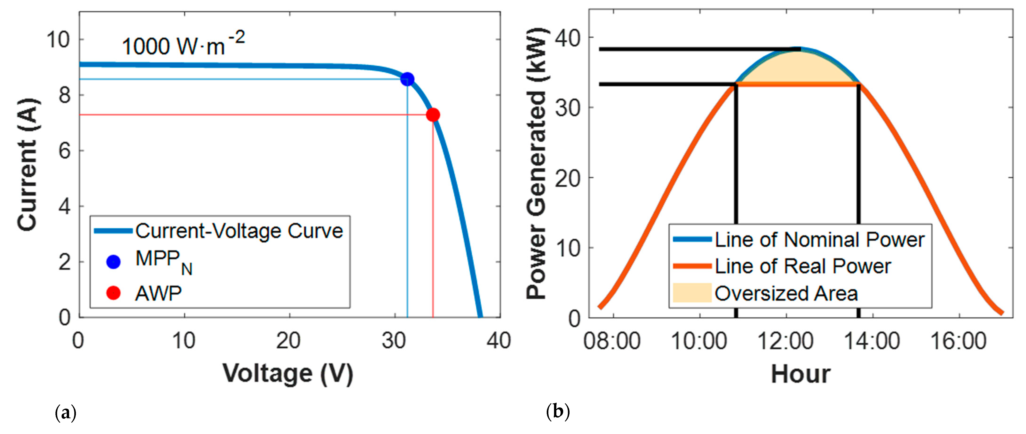
Usually, photovoltaic generators for solar pumping are oversized to guarantee the irrigation time, overcome highly variable irradiance, and compensate for the ageing of the modules, among other reasons. However, this oversizing has effects in their operation, which must be considered when simulating the system. The current photovoltaic models obtain results while working at the nominal point of maximum power (MPPN) of the Current-Voltage curve. However, oversizing of the photovoltaic generators causes the generator to work out of the MPPN, depending on the characteristics of the electrical system that limits the generator (Figure 2a,b). The actual working point (AWP) is controlled by the VFD. In the I-Solar model, a control algorithm of the power generated that considers generator oversizing can be used in the simulation process.
With the I-Solar model, these aspects have been considered, suggesting a clear improvement over current existing models. A new approach is provided to improve the model, which consists of obtaining a control algorithm for the generated power to determine the power that is provided by the photovoltaic generator in real operating conditions. To do this, the algorithm distinguishes between two zones with different operating behaviours. The first is where the photovoltaic power obtained is higher than that of the AWP, while the second is located between the AWP and the nominal power of VFD (POWVFD).
The control algorithm for the generated power continually checks the power generated by the photovoltaic generator to determine the zone where the value is located, and calculates the photovoltaic power in STC using the real irradiance at any given moment. Subsequently, Equation (22) establishes a relationship between the STC power achieved and the power corresponding to the study zone through use of the dimensionless coefficient “CA” which allows readjustment of the intensity according to the corresponding voltage value of the I-V curve defining the real maximum power achieved at each moment.
where POWSTC_i is the achieved power in STC according to the real irradiance at instant “i”, and POWS_A is the maximum power achieved according to the study zone.
In the case where the power obtained during the photovoltaic simulation is not located in the zones affected by oversizing, the algorithm does not provide any change in the initial power calculated. Therefore, the model I-Solar is prepared to detect both conditions automatically, with and without oversizing.
The manufacturers of photovoltaic modules guarantee a useful life of 25−30 years. However, each year the photovoltaic modules degrade with age, affecting their global efficiency. In this model, a polynomial function has been implemented (Equation (23)), based on values provided by the manufacturer of % efficiency loss between the first and final years of useful life guarantee, which allows the annual power losses in the photovoltaic modules to be calculated. Thus, in the model I-Solar it is only necessary to select the year of useful life of the photovoltaic modules (x) to obtain results.
The efficiency of the VFD was determined under highly variable environmental conditions (Equation (24)). With the values obtained, an adjustment with a second-degree polynomial was carried out. This parameter, which can only be obtained by measuring the power in DC and AC (before and after the VFD), is a key factor for the accurate simulation of solar pumping systems.
where ηVFD is the efficiency of VFD (%), POWAC is the output power of VFD in AC (kW), and POWDC the inlet power of VFD in DC (kW).
2.3.4. Simulation Model Based on Machine Learning, AI-Solar
Different types of machine learning were evaluated using massive data captured with the monitoring system described above. The Classification Learner application of Matlab® (Mathworks Inc., Natick, MA, USA) as well as the NETLAB library [60] for artificial neural networks in Matlab® were used with the aim of determining the most appropriate algorithm. The inlet variables in the model were global irradiance on the horizontal surface (W·m−2), ambient temperature (°C), and wind speed (m·s−1). The output variable was the power generated in AC (W). Table 4 shows the machine learning evaluation. Data were split into calibration (85%) and testing data (15%). In the calibration process, a cross-validation was performed using 5 folds. To select the best predictive model, the model performance was evaluated using testing data.
2.3.5. Statistical Analysis of the Evaluated Models
To analyze the goodness of fit of the model, a statistical analysis was performed based on the calculation of the root mean square error (RMSE), relative error (RE), and coefficient of determination (R2). Additionally, the adjustment to the normal of the residuals and homoscedasticity were also evaluated.
3. Results and Discussion
The results first show the statistical adjustment of the different models (simplified, I-Solar, and AI-Solar) to the measured data. Subsequently, the main variables that affect the performance of the models (cell temperature, control algorithm, and VFD efficiency) are analyzed.
3.1. Analysis of the Regression Models Based on Artificial Intelligence, AI-Solar Model
To determine the type of machine learning that represents the best operation of the photovoltaic system, the main statistical results were obtained for each of the machine learning types described in the methodology (Table 5).
The most accurate machine learning type was a Gaussian process regression (GPR) with exponential kernel function, with a relative error of 5.8%, a RMSE of 1226.7 W, and an R2 of 0.95. The poor performance of the linear regression models shows the complexity and non-linearity of the analyzed problem. The same result is observed when using a linear kernel in the SVM algorithms. However, the remaining algorithms that use non-linear kernels show adequate performance.
The implementation of machine learning algorithms requires the acquisition of massive data to calibrate and validate the model. Although the performance of the model is highly accurate, the generated model is specific to the system analyzed and cannot be applied to other photovoltaic systems.
3.2. Operation Analysis of the Developed Models
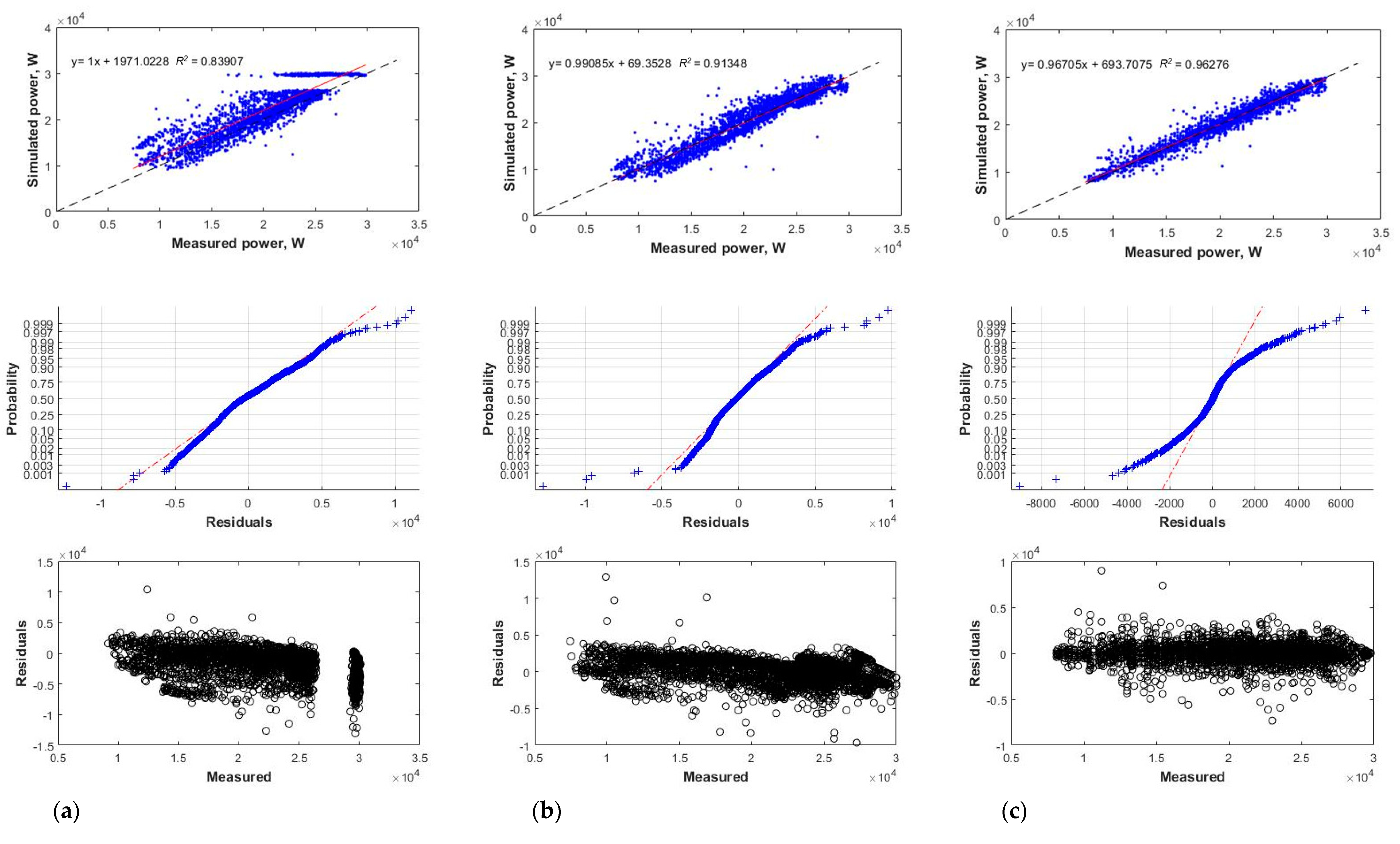
A comparison between the power values measured with the electrical network analyser at output VFD (in AC) and the evaluated models is shown in Figure 3: (1) simplified model, (2) I-Solar model, and (3) AI-Solar model. The statistical analysis is shown in Table 6. The developed AI-Solar model was trained with GPR-Exponential (GPR-E), which results in greater precision.
Of the models evaluated, the model based on machine learning, AI-Solar, shows the best adjustment. Models I-Solar and AI-Solar offer a clear improvement over the simplified model, decreasing the relative error of 14.2% for the simplified model to 7.5% and 5.8% for the proposed I-Solar and AI-Solar (artificial intelligence) models, respectively.
In addition, the results of the simplified model show a high spread of errors due to the overestimation both of the output power of the photovoltaic generator in DC and of the VFD, which was calculated based on empirical coefficients that led to the fixing of the maximum possible power of the VFD at 30 kW.
To determine the potential sources of error in the simplified model with respect to the parametric model I-Solar, the main variables that affect the simulation power have been analyzed, such as cell temperature, control of the generated power, and actual performance of the VFD.
3.3. Wind Speed Effect in Cell Temperature
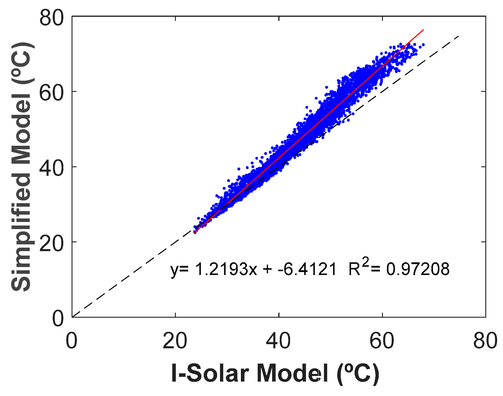
The cell temperature estimated by the I-Solar model is lower (Figure 4) because it considers wind speed and the resulting temperature decrease due to convection processes. It is observed that the largest differences are obtained for medium-high cell temperature values, with a maximum difference of up to 11 °C. The overestimation of the cell temperature can lead to an underestimation of the generated power. However, it has been concluded in Section 3.2. that the simplified model tends to overestimate the generated power, which confirms the lack of precision that the simplified model has in global terms. If a more accurate cell temperature was estimated by the simplified model, even higher inaccuracies of the model would have been apparent.
3.4. Effect of the Generated Power Control Algorithm
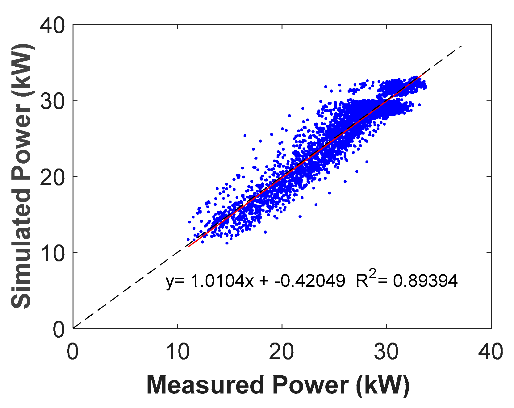
In common practical situations where the photovoltaic generator is oversized in the design phase, the generated power control algorithm results in an accurate estimation of the generated power for high irradiance values. In this case study, as an example for a representative period in summer (June, July, and August), this difference can reach up to 6.5 kW. Figure 5 presents the statistical adjustment, and Table 7 shows the statistical analysis, of the relationships between measured power and simulated power with the I-Solar model just downstream of the photovoltaic generator (in DC). The results indicate that, despite the slight differences in RMSE and R2 values compared to Table 6 (in AC), which may be due to the different precision of the measurement devices, there is a significant improvement in the relative error (RE).
As can be seen in Figure 5, high power values show a non-linear behaviour that reflects the zonal differentiation of the generated power control algorithm mentioned in the methodology section, which is also reflected in the measured values. The absence of their application in scenarios of oversizing leads to unfeasible results for any photovoltaic installation.
3.5. Influence of the Variable Frequency Drive (VFD) Efficiency
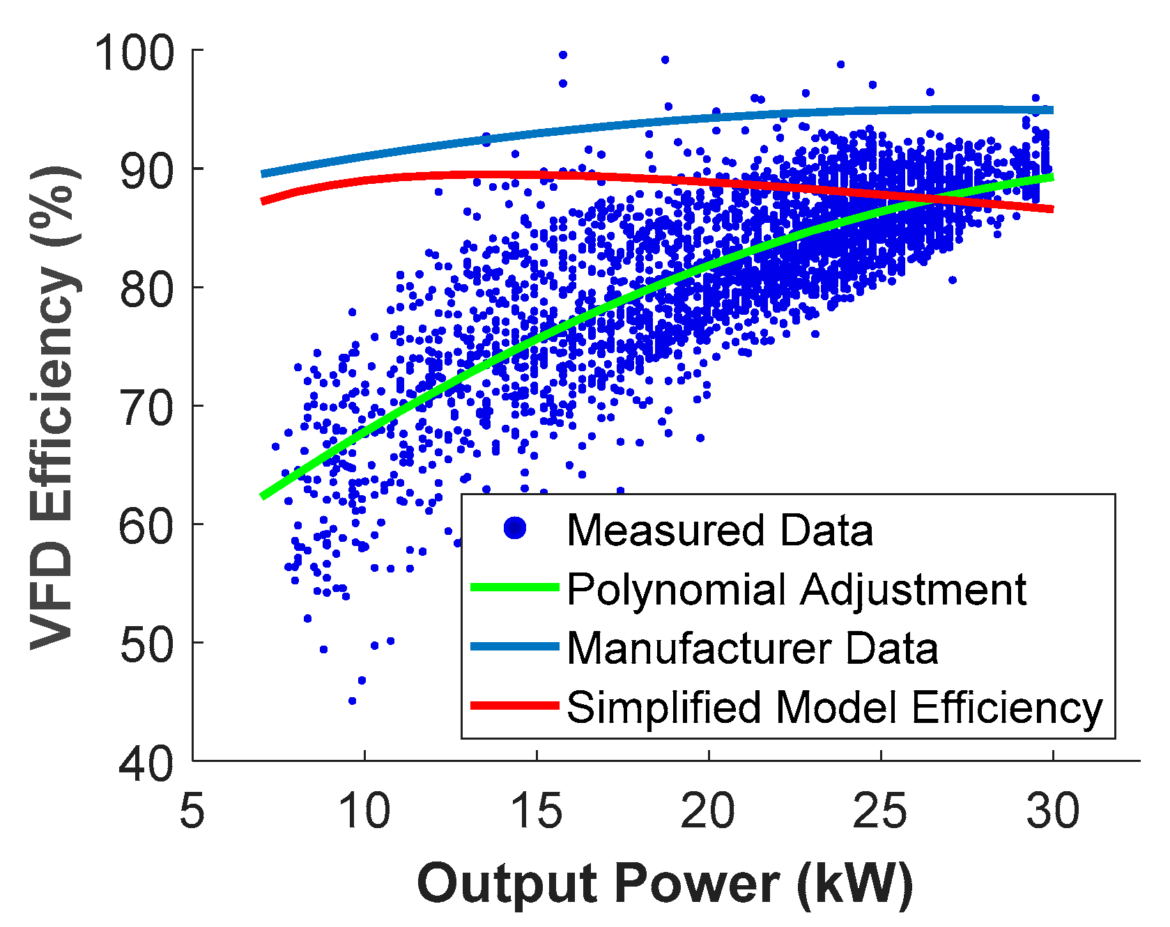
One of the key issues in accurately simulating a photovoltaic system to energize a pump using a VFD is estimating the efficiency of the VFD for any irradiance condition. In this case study, the adjustment curve of the VFD efficiency for the I-Solar model (ηVFD I-Solar) is shown in Figure 6 and Equation (25), using a second-degree polynomial equation depending on the output power in the VFD (x).
This methodology has been compared with parameters supplied by the VFD manufacturer. Figure 6 shows that the measured efficiency of the VFD at 30 kW reached a value of 90% while the value supplied by the manufacturer was close to 95%. All measured efficiency values were much lower than the efficiency specified by the manufacturer, with higher differences for low powers (consequently low frequencies). The large difference at low power values is significant. For example, at 7.5 kW, the manufacturer indicated a VFD efficiency of 89%, while the measured values only achieved a VFD efficiency of 57%. The high temperatures reached at the VFD locations is an important factor. It is important to consider that this equipment mainly works in the middle of the day in summer, where the temperature values inside the VFD electrical housing can become very high, even with adequate ventilation. The differences found indicate that it is necessary to characterize the actual efficiency of the VFD under real working conditions. In addition, it highlights the necessity of establishing an improved standard to determine the efficiency of these devices in non-ideal working conditions, primarily at high temperatures.
The comparison curve between the VDF efficiency supplied by the manufacturer and the VFD efficiency calculated for the simplified method, which was simulated using the general equation described in Section 2.3.2, is shown in Figure 6. The simulated values are seen to always be below the curve of the manufacturer, with an antagonistic trend with regard to measured values, and with an approximation at low powers, around 89% at 15.65 kW, while there is a decrease in the curve at medium power values which continues at high power values with a final efficiency of 86.5% at an output power of 30 kW. Thus, considering simplified solutions to take into account the VFD efficiency could lead to large inaccuracies in the final model.
4. Conclusions
This work examines fundamental issues to consider in the modelling of photovoltaic solar energy that are useful in the process of decision making for end users of this technology.
The complexity in the development of photovoltaic system tools and models is affected by the strong influence of the parameters involved during the process. Collecting large amounts of real-world measured values have allowed us to describe the performance of the photovoltaic installation, allowing the generation of an accurate and sturdy I-Solar model that efficiently integrates all influential stages in photovoltaic production through the application of methodologies from different studies as well as new developments in this study. The model has been validated with measured values to manage the system in real time.
Although solar pumping systems are discussed in this work, this model can be integrated into any type of photovoltaic system, such as solar pumping systems or grid connected systems, which provide high versatility and utility.
The parametric I-Solar model developed to determine the electric power generated in photovoltaic solar systems has allowed us to obtain a similar precision (RE = 7.5%) to the non-parametric model (RE = 5.8%) based on machine learning. The simplicity of the parametric simplified model results in a clear lack of precision (RE = 14.2%). In addition, parametric models are of general application for any photovoltaic solar installation, while the non-parametric models are specific to each installation and require a large number of values derived from the monitoring systems.
Solar radiation values, which are the base element for the calculation of the photovoltaic production, are essential to achieve good integration in the calculation of the irradiance components that allows us to obtain the irradiance on an inclined surface in real time.
The effect of wind speed on the cell temperature has been demonstrated. It decreases the temperature by convection processes and consequently increases the module efficiency. Thus, the I-Solar generated model includes this variable compared to the simplified model.
The oversizing of the photovoltaic generator contributes to an increase in the generated power. However, it has been demonstrated that the incorporation of the generated power control algorithm in installations with these characteristics is essential to determine with precision the power used in real time in order to manage the system appropriately.
The need to characterize the VFD efficiency in real time has been demonstrated because of the significant differences between values supplied by the manufacturer and the measured values, which affect the generated power and consequently the system management.
The current capacity for monitoring photovoltaic systems allows us to obtain large amounts of performance data from these systems that can be used in machine learning to establish accurate relationships with the final generation of electric energy. Most of these studies are focused on the prediction of photovoltaic energy generation, while the objective of this work is to determine the power generated in real time. In addition, these models are useful for generating alarms when the measured power is significantly different to the power simulated by the system.
The level of precision obtained with the I-Solar model can be useful in decision-making to determine the optimal technical and economic specifications of photovoltaic solar installations.
Author Contributions
Conceptualization, M.A.M.; methodology, J.C.-G., J.M. and M.A.M.; software, J.C.-G.; validation, J.C.-G., J.M. and M.A.M.; formal analysis, J.M. and M.A.M.; investigation, J.C.-G., J.M. and M.A.M.; resources, J.C.-G.; data curation, J.C.-G.; writing—original draft preparation, J.C.-G.; writing—review and editing, J.C.-G., J.M. and M.A.M.; visualization, J.M.; supervision, J.M. and M.A.M.; project administration, M.A.M.; funding acquisition, M.A.M. All authors have read and agreed to the published version of the manuscript.
Funding
This research was funded by the Spanish Ministry of Education and Science (MEC), grant number AGL2017-82927-C3-2-R (co-funded by FEDER) and the University of Castilla-La Mancha predoctoral grant action. We would like to thank Juan José Toboso, the owner of the Peruelos farm, for his unlimited help to us when carrying out this work. We would also like to thank the U.S. Sandia National Laboratories and the U.S. National Renewable Energy Laboratory (NREL) for their support and information, which made it possible to develop these models.
Institutional Review Board Statement
Not applicable.
Informed Consent Statement
Not applicable.
Data Availability Statement
Data sharing not applicable.
Conflicts of Interest
The authors declare no conflict of interest.
Nomenclature
| a | Ideality Factor (V) | Nm | Number of modules in series |
| a’ | Coefficient to determinate Vmax and Imax | NOCT | Nominal Operating Cell Temperature |
| AC | Alternate current | POWAC | VFD output power in AC (kW) |
| AI | Artificial Intelligence | POWDC | VFD inlet power in DC (kW) |
| Al | Aluminium | PowMAX_G | Maximum power photovoltaic generator (kW) |
| AWP | Actual working point | POWS_A | Maximum power according study area (kW) |
| b | Coefficient to determinate Vmax and Imax | POWSTC_i | STC power of real irradiance in an instant “i” (kW) |
| CA | Dimensionless coefficient | POWVFD | VFD nominal power (kW) |
| CLPOW | Power losses in cables (kW) | PVGIS | Photovoltaic Geographical Information System |
| Cu | Copper | R | Resistance according temperature (Ω) |
| DC | Direct current | R2 | Coefficient of determination |
| DHI | Diffuse irradiance on horizontal surface (W·m−2) | RE | Relative Error |
| DHIT | Diffuse irradiance on inclined surface (W·m−2) | REn | Renewable energy |
| DISC | Direct Insolation Simulation Code | RIT | Reflected irradiance on inclined surface (W·m−2) (W·m−2) |
| DNI | Direct normal irradiance on horizontal surface (W·m−2) | RMSE | Root Mean Square Error |
| DNIT | Direct normal irradiance on inclined surface (W·m−2) | rs | Normalized resistance |
| E | Incident solar irradiance (W·m−2) | RS | Series Resistance (Ohm) |
| Eo | Reference solar irradiance (1000 W·m−2) | Rsh | Parallel Resistance (Ohm) |
| FFO | Ideal cell fill factor | s | Section of the cable (mm2) |
| FFSTC | Fill factor in standard test conditions | STC | Standard Test Condition |
| G | Irradiance (W·m−2) | SVM | Support Vector Machine |
| GHG | Greenhouse gases | Ta | Ambient temperature (°C) |
| GHI | Global irradiance on horizontal surface (W·m−2) | TC | Cell temperature (°C) |
| GIT | Total irradiance on inclined surface (W·m−2) | Tm | Photovoltaic module temperature (°C) |
| GPR-E | Gaussian process regression-Exponential | VD | Voltage drop (V) |
| I | Current in the cable (A) | ηVFDSimplified | VFD efficiency in the simplified model (%) |
| IL | Light Generated Current (A) | VFD | Variable frequency drive |
| IMAX | Current at point of maximum power (A) | VMAX | Voltage at point of maximum power (V) |
| lmpp | Current at point of maximum power in STC(A) | Vmpp | Voltage at point of maximum power in STC (V) |
| Imax | AC current in the cable (A) | Voc | Open circuit voltage (V) |
| Io | Dark Saturation Current (A) | Vt | Thermal voltage (V) |
| ISC | Short circuit current (A) | ΔT | Difference of temperature between the cell and the back surface of the photovoltaic module |
| k0, k1, k2 | Coefficients of characteristic losses for VFD | ηVFD | Efficiency of VFD (%) |
| kWp | Kilowatt peak | θz | Solar zenith angle |
| L | Length of the cable (m) | ξ | Incidence angle of the sun rays on the inclined surface |
| MPPN | Nominal point of maximum power (kW) | σz | Solar zenith angle |
| N | Number of conductors | β | Angle on inclined surface |
| Ncp | Number of cells in parallel | ρ | Albedo |
| Ncs | Number of cells in series | Normalized cell voltage | |
| Nmp | Number of modules in parallel | σ | Conductivity of the material (m·Ω−1·mm−2) |
References
- Capellán-Pérez, I.; Mediavilla, M.; de Castro, C.; Carpintero, Ó.; Miguel, L.J. Fossil fuel depletion and socio-economic scenarios: An integrated approach. Energy 2014, 77, 641–666. [Google Scholar] [CrossRef]
- Wang, J.; Feng, L.; Tang, X.; Bentley, Y.; Höök, M. The implications of fossil fuel supply constraints on climate change projections: A supply-side analysis. Futures 2017, 86, 58–72. [Google Scholar] [CrossRef]
- Kelley, L.C.; Gilbertson, E.; Sheikh, A.; Eppinger, S.D.; Dubowsky, S. On the feasibility of solar-powered irrigation. Renew. Sustain. Energy Rev. 2010. [Google Scholar] [CrossRef]
- IRENA. Future of Solar PV Summary 2019; IRENA: Abu Dabi, United Arab Emirates, 2019. [Google Scholar]
- Burney, J.; Woltering, L.; Burke, M.; Naylor, R.; Pasternak, D. Solar-powered drip irrigation enhances food security in the Sudano-Sahel. Proc. Natl. Acad. Sci. USA 2010, 107, 1848–1853. [Google Scholar] [CrossRef] [Green Version]
- Dursun, M.; Ozden, S. Application of Solar Powered Automatic Water Pumping in Turkey. Int. J. Comput. Electr. Eng. 2012, 4, 161–164. [Google Scholar] [CrossRef] [Green Version]
- Vartiainen, E.; Masson, G.; Breyer, C.; Moser, D.; Román Medina, E. Impact of weighted average cost of capital, capital expenditure, and other parameters on future utility-scale PV levelised cost of electricity. Prog. Photovolt. Res. Appl. 2020, 28, 439–453. [Google Scholar] [CrossRef] [Green Version]
- Jäger-Waldau, A. PV Status Report 2019; European Commission: Brussels, Belgium, 2019. [Google Scholar]
- Wu, C.; Chen, C.; Tao, L.; Ding, X.; Zheng, M.; Li, H.; Li, G.; Lu, H.; Cheng, M. Highly efficient perovskite solar cells based on symmetric hole transport material constructed with indaceno[1,2-b:5,6-b’]dithiophene core cuilding clock. J. Energy Chem. 2020, 43, 98–103. [Google Scholar] [CrossRef] [Green Version]
- Olczak, P.; Olek, M.; Matuszewska, D.; Dyczko, A.; Mania, T. Monofacial and Bifacial Micro PV Installation as Element of Energy Transition—The Case of Poland. Energies 2021, 14, 499. [Google Scholar] [CrossRef]
- Pascaris, A.S.; Schelly, C.; Pearce, J.M. A First Investigation of Agriculture Sector Perspectives on the Opportunities and Barriers for Agrivoltaics. Agronomy 2020, 10, 1885. [Google Scholar] [CrossRef]
- Tarjuelo, J.M.; Rodriguez-Diaz, J.A.; Abadía, R.; Camacho, E.; Rocamora, C.; Moreno, M.A. Efficient water and energy use in irrigation modernization: Lessons from Spanish case studies. Agric. Water Manag. 2015, 162, 67–77. [Google Scholar] [CrossRef]
- Jackson, T.M.; Khan, S.; Hafeez, M. A comparative analysis of water application and energy consumption at the irrigated field level. Agric. Water Manag. 2010, 97, 1477–1485. [Google Scholar] [CrossRef]
- Moreno, M.A.; Ortega, J.F.; Córcoles, J.I.; Martínez, A.; Tarjuelo, J.M. Energy analysis of irrigation delivery systems: Monitoring and evaluation of proposed measures for improving energy efficiency. Irrig. Sci. 2010, 28, 445–460. [Google Scholar] [CrossRef]
- Izquiel, A.; Ballesteros, R.; Tarjuelo, J.M.; Moreno, M.A. Optimal reservoir sizing in on-demand irrigation networks: Application to a collective drip irrigation network in Spain. Biosyst. Eng. 2016, 147. [Google Scholar] [CrossRef]
- Todde, G.; Murgia, L.; Deligios, P.A.; Hogan, R.; Carrelo, I.; Moreira, M.; Pazzona, A.; Ledda, L.; Narvarte, L. Energy and environmental performances of hybrid photovoltaic irrigation systems in Mediterranean intensive and super-intensive olive orchards. Sci. Total Environ. 2019, 651, 2514–2523. [Google Scholar] [CrossRef]
- Capellán-Pérez, I.; Campos-Celador, Á.; Terés-Zubiaga, J. Renewable Energy Cooperatives as an instrument towards the energy transition in Spain. Energy Policy 2018, 123, 215–229. [Google Scholar] [CrossRef]
- Aliyu, M.; Hassan, G.; Said, S.A.; Siddiqui, M.U.; Alawami, A.T.; Elamin, I.M. A review of solar-powered water pumping systems. Renew. Sustain. Energy Rev. 2018, 87, 61–76. [Google Scholar] [CrossRef]
- Vick, B.; Neal, B.; Clark, R.; Holman, A. Water Pumping with AC Motors and Thin-Film Solar Panels. In Proceedings of the 32nd ASES Annual Conference; American Solar Energy Society: Austin, TX, USA, 2003; p. 6. [Google Scholar]
- Pande, P.C.; Singh, A.K.; Ansari, S.; Vyas, S.K.; Dave, B.K. Design development and testing of a solar PV pump based drip system for orchards. Renew. Energy 2003, 28, 385–396. [Google Scholar] [CrossRef]
- Senol, R. An analysis of solar energy and irrigation systems in Turkey. Energy Policy 2012, 47, 478–486. [Google Scholar] [CrossRef]
- Reca, J.; Torrente, C.; López-Luque, R.; Martínez, J. Feasibility analysis of a standalone direct pumping photovoltaic system for irrigation in Mediterranean greenhouses. Renew. Energy 2016, 85, 1143–1154. [Google Scholar] [CrossRef] [Green Version]
- Bouzidi, B. Viability of solar or wind for water pumping systems in the Algerian Sahara regions—Case study Adrar. Renew. Sustain. Energy Rev. 2011, 15, 4436–4442. [Google Scholar] [CrossRef]
- Cervera-Gascó, J.; Montero, J.; Del Castillo, A.; Tarjuelo, J.M.; Moreno, M.A. EVASOR, an integrated model to manage complex irrigation systems energized by photovoltaic generators. Agronomy 2020, 10, 331. [Google Scholar] [CrossRef] [Green Version]
- Ibrik, I. Micro-grid solar photovoltaic systems for rural development and sustainable agriculture in palestine. Agronomy 2020, 10, 1474. [Google Scholar] [CrossRef]
- Lorenzo, C.; Almeida, R.H.; Martínez-Núñez, M.; Narvarte, L.; Carrasco, L.M. Economic assessment of large power photovoltaic irrigation systems in the ECOWAS region. Energy 2018, 155, 992–1003. [Google Scholar] [CrossRef]
- Liu, B.Y.H.; Jordan, R.C. The interrelationship and characteristic distribution of direct, diffuse and total solar radiation. Sol. Energy 1960, 4, 1–19. [Google Scholar] [CrossRef]
- Collares-Pereira, M.; Rabl, A. The average distribution of solar radiation-correlations between diffuse and hemispherical and between daily and hourly insolation values. Sol. Energy 1979, 22, 155–164. [Google Scholar] [CrossRef]
- Erbs, D.G.; Klein, S.A.; Duffie, J.A. Estimation of the diffuse radiation fraction for hourly, daily and monthly-average global radiation. Sol. Energy 1982, 28, 293–302. [Google Scholar] [CrossRef]
- Muneer, T. Solar radiation model for Europe. Build. Serv. Eng. Res. Technol. 1990, 11, 153–163. [Google Scholar] [CrossRef]
- Duffie, J.A.; Beckman, W.A. Solar Engineering of Thermal Processes, 3rd ed.; Wiley: Hoboken, NJ, USA, 2006; ISBN 978-0-471-69867-8. [Google Scholar]
- Shen, C.; He, Y.L.; Liu, Y.W.; Tao, W.Q. Modelling and simulation of solar radiation data processing with Simulink. Simul. Model. Pract. Theory 2008, 16, 721–735. [Google Scholar] [CrossRef]
- Perez, R.; Ineichen, P.; Seals, R.; Michalsky, J.; Stewart, R. Modeling daylight availability and irradiance components from direct and global irradiance. Sol. Energy 1990, 44, 271–289. [Google Scholar] [CrossRef] [Green Version]
- Gracia, A.M.; Huld, T. Performance Comparison of Different Models for the Estimation of Global Irradiance on Inclined Surfaces; European Comission: Luxemburg, 2013. [Google Scholar]
- Evseev, E.G.; Kudish, A.I. The assessment of different models to predict the global solar radiation on a surface tilted to the south. Sol. Energy 2009, 83, 377–388. [Google Scholar] [CrossRef]
- Green, M.A. Accuracy of analytical expressions for solar cell fill factors. Sol. Cells 1982, 7, 337–340. [Google Scholar] [CrossRef]
- Blaesser, G.; Rossi, E. Extrapolation of outdoor measurements of PV array I-V characteristics to standard test conditions. Sol. Cells 1988, 25, 91–96. [Google Scholar] [CrossRef]
- Marion, B. A method for modeling the current-voltage curve of a PV module for outdoor conditions. Prog. Photovolt. Res. Appl. 2002, 10, 205–214. [Google Scholar] [CrossRef]
- Abete, A.; Napoli, R.; Spertino, F.A. A simulation procedure to predict the monthly energy supplied by grid connected PV systems. In Proceedings of the 3rd World Conference on Photovoltaic Energy Conversion, Osaka, Japan, 11–18 May 2003. [Google Scholar]
- Zerhouni, F.Z.; Zerhouni, M.H.; Zegrar, M.; Benmessaoud, M.T.; Stambouli, A.B.; Midoun, A. Proposed methods to increase the output efficiency of a photovoltaic (PV) system. Acta Polytech. Hung. 2010, 7, 55–70. [Google Scholar]
- López-Luque, R.; Reca, J.; Martínez, J. Optimal design of a standalone direct pumping photovoltaic system for deficit irrigation of olive orchards. Appl. Energy 2015, 149, 13–23. [Google Scholar] [CrossRef]
- Mérida García, A.; Fernández García, I.; Camacho Poyato, E.; Montesinos Barrios, P.; Rodríguez Díaz, J.A. Coupling irrigation scheduling with solar energy production in a smart irrigation management system. J. Clean. Prod. 2018, 175, 670–682. [Google Scholar] [CrossRef]
- Aguilar, J.; Pérez-Higueras, P.; Almonacid, G. Average power of a photovoltaic grid-connected system. In Proceedings of the World Renewable Energy Congress IX, Florence, Italy, 19–25 August 2006. [Google Scholar]
- Jain, A.; Kapoor, A. A new method to determine the diode ideality factor of real solar cell using Lambert W-function. Sol. Energy Mater. Sol. Cells 2005, 85, 391–396. [Google Scholar] [CrossRef]
- Bellia, H.; Youcef, R.; Fatima, M. A detailed modeling of photovoltaic module using MATLAB. NRIAG J. Astron. Geophys. 2014, 3, 53–61. [Google Scholar] [CrossRef] [Green Version]
- Chouder, A.; Silvestre, S.; Sadaoui, N.; Rahmani, L. Modeling and simulation of a grid connected PV system based on the evaluation of main PV module parameters. Simul. Model. Pract. Theory 2012, 20, 46–58. [Google Scholar] [CrossRef]
- Bishop, C. Neural Networks for Pattern Recognition; Oxford University Press: Cambridge, UK, 1995; Volume 1995, ISBN 9780198538646. [Google Scholar]
- Ibrahim, I.A.; Khatib, T.; Mohamed, A.; Elmenreich, W. Modeling of the output current of a photovoltaic grid-connected system using random forests technique. Energy Explor. Exploit. 2018, 36, 132–148. [Google Scholar] [CrossRef] [Green Version]
- Antonanzas, J.; Osorio, N.; Escobar, R.; Urraca, R.; Martinez-de-Pison, F.J.; Antonanzas-Torres, F. Review of photovoltaic power forecasting. Sol. Energy 2016, 136, 78–111. [Google Scholar] [CrossRef]
- Moreno, M.A.; Carrión, P.A.; Planells, P.; Ortega, J.F.; Tarjuelo, J.M. Measurement and improvement of the energy efficiency at pumping stations. Biosyst. Eng. 2007, 98, 479–486. [Google Scholar] [CrossRef]
- Maxwell, E.L. A Quasi-Physical Model for Converting Hourly Global Horizontal to Direct Normal lnsolation; Solar Energy Research Institute: Golden, CO, USA, 1987. [Google Scholar]
- Perez, R.; Ineichen, E.P.; Maxwell, R.S.; Zelenka, A. Dynamic global-to-direct irradiance conversion models. ASHRAE Trans. Ser. 1992, 98, 354–369. [Google Scholar]
- Labouret, A.; Villoz, M. Energie Solaire Photovoltaïque; Dunod, L.M., Ed.; Technique et Ingénierie—Environnement et Sécurité; Dunod: Malakoff, France, 2006; ISBN 978-2-10-049945-8. [Google Scholar]
- Mohammed, S.S. Modeling and Simulation of Photovoltaic module using MATLAB/Simulink. Int. J. Chem. Environ. Eng. 2011, 2, 6. [Google Scholar]
- Jantsch, M.; Schimidt, H.; Schmid, J. Results of the Concerted Action on Power Conditioning and control. In Proceedings of the 11th European Photovoltaic Solar Energy Conference, Montreux, Switzerland, 12–16 October 1992; pp. 1589–1592. [Google Scholar]
- De Soto, W.; Klein, S.A.; Beckman, W.A. Improvement and validation of a model for photovoltaic array performance. Sol. Energy 2006, 80, 78–88. [Google Scholar] [CrossRef]
- Minemoto, T.; Nagae, S.; Takakura, H. Impact of spectral irradiance distribution and temperature on the outdoor performance of amorphous Si photovoltaic modules. Sol. Energy Mater. Sol. Cells 2007, 91, 919–923. [Google Scholar] [CrossRef]
- Minemoto, T.; Fukushige, S.; Takakura, H. Difference in the outdoor performance of bulk and thin-film silicon-based photovoltaic modules. Sol. Energy Mater. Sol. Cells 2009, 93, 1062–1065. [Google Scholar] [CrossRef]
- King, D.L.; Boyson, W.E.; Kratochvill, J.A. Photovoltaic Array Performance Model; Sandia National Laboratories: Albuquerque, NM, USA, 2004. [Google Scholar] [CrossRef] [Green Version]
- Nabney, I. Netlab: Algorithms for Pattern Recognition; Springer: Berlin/Heidelberg, Germany, 2002; ISBN 1-85233-440-1. [Google Scholar]
Figure 1.
(a) Location of the pyranometer and agro-climatic station and (b) Location of the electrical network analysers in the inlet and output of the variable frequency drive (VFD).
Figure 1.
(a) Location of the pyranometer and agro-climatic station and (b) Location of the electrical network analysers in the inlet and output of the variable frequency drive (VFD).

Figure 2.
(a) Current-Voltage curve and nominal and real points of maximum power (MPPN and AWP of operation and (b) example of power generated by the photovoltaic generator. MPPN: nominal point of maximum power operation. AWP: actual working point.
Figure 2.
(a) Current-Voltage curve and nominal and real points of maximum power (MPPN and AWP of operation and (b) example of power generated by the photovoltaic generator. MPPN: nominal point of maximum power operation. AWP: actual working point.

Figure 3.
Statistical adjustment of the Simplified Model (a), I-Solar model (b) and AI-Solar model (c), adjustment to the normal of the normal of the residuals and homoscedasticity.
Figure 3.
Statistical adjustment of the Simplified Model (a), I-Solar model (b) and AI-Solar model (c), adjustment to the normal of the normal of the residuals and homoscedasticity.

Figure 4.
Comparison of estimated cell temperature between simplified and I-Solar model.

Figure 5.
Statistical adjustment of the I-Solar model in direct current (DC).

Figure 6.
Comparison between the VFD efficiency supplied by the manufacturer, the VFD efficiency measured and the VFD efficiency obtained through the general equation of the simplified method.
Figure 6.
Comparison between the VFD efficiency supplied by the manufacturer, the VFD efficiency measured and the VFD efficiency obtained through the general equation of the simplified method.


Table 1.
Technical characteristics of the photovoltaic modules.
| Technical Characteristics | Value | Unit |
|---|---|---|
| Maximum Power in STC | 265 | Wp |
| Voltage at point of maximum power (Vmpp) in STC | 31.16 | V |
| Current at point of maximum power (lmpp) in STC | 8.57 | A |
| Open circuit voltage (Voc) in STC | 38.12 | V |
| Short circuit current (Isc) in STC | 9.01 | A |
| Efficiency | 16.2 | % |
| Power temperature coefficient | −0.42 | %/K |
| Current temperature coefficient | 0.059 | %/K |
| Voltage temperature coefficient | −0.32 | %/K |
| Nominal Operating Cell Temperature (NOCT) | 46 ± 2 | °C |
| Cell type | polycrystalline silicon | |
| Number of cells | 60 | |
STC: Standard Test Condition (Irradiance of 1000 W·m−2, Cell temperature of 25 °C, AM 1.5 Spectrum); NOCT: Nominal Operating Cell Temperature (Irradiance of 800 W·m−2, Ambient temperature of 20 °C, Wind speed of 1 ms−1).
Table 2.
Lines of cables.
| Line | Total Length (m) | Section (mm2) | Material |
|---|---|---|---|
| (1) Photovoltaic Generator (PG) | 252.5 | 4 | Cu |
| (2) PG-variable frequency drive (VFD) | 10 | 25 | Cu |
| (3) VFD–Borehole inlet (BI) | 470 | 150 | Al |
| (4) BI-submersible motor | 225 | 25 | Cu |
Cu: copper; Al: aluminium.
Table 3.
Characteristics of the photovoltaic module Astronergy Solarmodule ASM6610P 265, provided by US Sandia National Laboratories and US National Renewable Energy Laboratory (NREL).
Table 3.
Characteristics of the photovoltaic module Astronergy Solarmodule ASM6610P 265, provided by US Sandia National Laboratories and US National Renewable Energy Laboratory (NREL).
| Characteristic | Value | Unit |
|---|---|---|
| Ideality Factor (a) | 1.540 | V |
| Light Generated Current (IL) | 9.106 | A |
| Dark Saturation Current (Io) | 1.59 × 10⁻¹⁰ | A |
| Series Resistance (RS) | 0.275 | Ohm |
| Parallel Resistance (Rsh) | 409.580 | Ohm |
Table 4.
Machine learning algorithms evaluated.
| Group | Method | Id. |
|---|---|---|
| Linear Regression | Linear Regression | LR |
| Interactions Linear | IL | |
| Robust Linear | RL | |
| Decision Trees | Fine Tree | FT |
| Medium Tree | MT | |
| Coarse Tree | CT | |
| Support Vector Machines | Linear SVM | SVM-L |
| Quadratic SVM | SVM-Q | |
| Cubic SVM | SVM-C | |
| Fine Gaussian SVM | SVM-FG | |
| Medium Gaussian SVM | SVM-MG | |
| Coarse Gaussian SVM | SVM-CG | |
| Gaussian Process Regression | Rational Quadratic | GPR-RQ |
| Squared Exponential | GPR-SE | |
| Matern 5/2 | GPR-M | |
| Exponential | GPR-E | |
| Ensemble Classifiers | Boosted Trees | E-BoT |
| Bagged Trees | E-BaT | |
| Artificial Neural Network | Back Propagation | ANN |
Table 5.
Main statistical results for machine learning using testing data.
| Model | RMSE (W) | RE (%) | R2 |
|---|---|---|---|
| LR | 1596.4 | 7.5 | 0.91 |
| IL | 1491.4 | 7.0 | 0.92 |
| RL | 1595.0 | 7.5 | 0.91 |
| FT | 1343.6 | 6.3 | 0.94 |
| MT | 1428.9 | 6.7 | 0.93 |
| CT | 1396.3 | 6.6 | 0.93 |
| SVM-L | 1602.1 | 7.5 | 0.91 |
| SVM-Q | 1346.9 | 6.3 | 0.93 |
| SVM-C | 1331.9 | 6.3 | 0.94 |
| SVM-FG | 1369.7 | 6.4 | 0.93 |
| SVM-MG | 1273.1 | 6.0 | 0.94 |
| SVM-CG | 1343.6 | 6.3 | 0.94 |
| GPR-RQ | 1245.7 | 5.8 | 0.94 |
| GPR-SE | 1268.6 | 6.0 | 0.94 |
| GPR-M | 1253.6 | 5.9 | 0.94 |
| GPR-E | 1226.7 | 5.8 | 0.95 |
| E-BoT | 1632.6 | 7.7 | 0.94 |
| E-BaT | 1331.5 | 6.3 | 0.94 |
| ANN | 1332.2 | 6.3 | 0.94 |
Table 6.
Statistical analysis of adjustment of the evaluated models.
| Model | RMSE (W) | RE (%) | R2 |
|---|---|---|---|
| Simplified | 3024.8 | 14.2 | 0.84 |
| I-Solar | 1602.8 | 7.5 | 0.91 |
| AI-Solar | 1226.7 | 5.8 | 0.95 |
Table 7.
Statistical analysis of the I-Solar model in DC.
| Model | RMSE (W) | RE (%) | R2 |
|---|---|---|---|
| I-Solar | 1750 | 6.83 | 0.89 |
Publisher’s Note: MDPI stays neutral with regard to jurisdictional claims in published maps and institutional affiliations. |
© 2021 by the authors. Licensee MDPI, Basel, Switzerland. This article is an open access article distributed under the terms and conditions of the Creative Commons Attribution (CC BY) license (http://creativecommons.org/licenses/by/4.0/).
Share and Cite
MDPI and ACS Style
Cervera-Gascó, J.; Montero, J.; Moreno, M.A. I-Solar, a Real-Time Photovoltaic Simulation Model for Accurate Estimation of Generated Power. Agronomy 2021, 11, 485. https://doi.org/10.3390/agronomy11030485
AMA Style
Cervera-Gascó J, Montero J, Moreno MA. I-Solar, a Real-Time Photovoltaic Simulation Model for Accurate Estimation of Generated Power. Agronomy. 2021; 11(3):485. https://doi.org/10.3390/agronomy11030485
Chicago/Turabian StyleCervera-Gascó, Jorge, Jesús Montero, and Miguel A. Moreno. 2021. "I-Solar, a Real-Time Photovoltaic Simulation Model for Accurate Estimation of Generated Power" Agronomy 11, no. 3: 485. https://doi.org/10.3390/agronomy11030485
Note that from the first issue of 2016, this journal uses article numbers instead of page numbers. See further details here.