Article

Modifying the CROPGRO Safflower Model to Simulate Growth, Seed and Floret Yield under Field Conditions in Southwestern Germany

by
Kathrin Steberl
1,*,
Kenneth J. Boote
2,
Sebastian Munz
1 and
Simone Graeff-Hönninger
1
1
Institute of Crop Science, University of Hohenheim, 70599 Stuttgart, Germany
2
Agricultural and Biological Engineering Department, University of Florida, Gainesville, FL 32611, USA
*
Author to whom correspondence should be addressed.
Agronomy 2020, 10(1), 11; https://doi.org/10.3390/agronomy10010011
Submission received: 11 October 2019 / Revised: 11 December 2019 / Accepted: 16 December 2019 / Published: 19 December 2019

Abstract

:
The Decision Support System for Agrotechnology Transfer (DSSAT) currently provides a safflower model based on CROPGRO. The model was calibrated with the field data of one cultivar grown in New Mexico in 2013 and 2014. As it is rather new and has not yet been tested with other field data, it is important to evaluate the model in different environments. This study evaluated the CROPGRO safflower model for two different cultivars grown under field conditions in southwestern Germany. In addition, a new approach was added, enabling it to predict the yield of florets, which is of special interest, as these are used as a food colorant in Europe. The default model was evaluated with data from 2017 and 2018, obtained in a field trial in southwestern Germany with two cultivars, with row spacing of 12 and 33 cm and sowing densities of 40 and 75 plants m−2. As the default model was not well adapted to European conditions, model modifications were implemented in the species, ecotype, and cultivar files. With these modifications, observed variables such as leaf appearance over time were well predicted (RMSE: 4.76; d-index: 0.88), and simulations of the specific leaf area and leaf area index were greatly improved (RMSE: 24.14 and 0.82; d-index: 0.78 and 0.73). Simulations of the original New Mexico data set were also improved. The newly-added approach to predict floret yield was successfully integrated into the model. Over two years and two cultivars, floret yield was simulated with a RMSE of 97.24 and a d-index of 0.79. Overall, the extended model proved to be useful for simulating growth, floret yield, and yield of safflower in southwestern Germany.

1. Introduction

Safflower (Carthamus tinctorius L.) is a member of the Compositae family, and has a long tradition of use by humans, mainly for its high quality oil, which includes highly polyunsaturated fatty acids [1,2,3,4,5]. It is also used as a medicinal plant, bird seed, cut flowers, livestock forage, and tea [1,3,6,7]. Additionally, it has traditionally been used as a colorant for textiles and food [1,2,3]. Today, China still cultivates safflower for its flowers, but on an international level, the importance of this sector is very small [3].
Different studies claim that there is a general negative influence of artificial food colorants on the behavior of children, regardless of whether they have attention-deficit/hyperactivity disorder (ADHD) or not [8,9]. Based on this concern and the general demand for healthier foods, interest in natural dyes is growing today, and the natural colorant business, especially in the food coloring sector, is continuing to grow worldwide [10,11,12,13]. In many countries, the yellow colorants of safflower are being increasingly used in the food and beverage industry for coloring fruit juice, fruit syrup, candies, or pastries [7,14,15,16]. The yellow pigment of safflower is cheaper than saffron, highly soluble in water, can be used at different temperatures and pH values, and is stable to light in aqueous solutions [7,14,15,16].
Due to the increasing demands of the food industry, the florets for colorant production have mainly been imported from Asia, where most safflower is produced [3,17]. However, this leads to problems such as delivery difficulties or pesticide residues. Studies have shown that safflower cultivars can be grown in Central European conditions [18,19,20,21,22]. However, these studies have been carried out for the production of seeds for the oil industry. None of these cultivars has been tested for their production of florets. In order to guide farmers to adopt new production systems or new directions of use, field trials need to be carried out to develop the appropriate guidelines.
Field trials are complex, very specific to a given site and season, and cost- and labor-intensive [23]. Crop growth modeling is a useful tool in research to simulate growth and potential yield [23,24]. One plant simulation model that has been used by many scientists worldwide for many years is the Decision Support System for Agrotechnology Transfer (DSSAT) [23,25]. In DSSAT, information on the weather, soil, crop/cultivar traits, and experimental data are used to simulate the growth and yields of different crops [23,24]. The DSSAT software [23] includes models for many crops following two types of templates, CERES and CROPGRO, where the latter uses a single common computer code plus read-in text files for species, ecotype, and cultivar parameters, which allows it to be adapted to a number of crops such as fababean [26], and more recently, safflower [27] and quinoa [28]. The existing model for safflower was developed to predict the safflower seed yield of one cultivar grown under four different irrigation treatments in New Mexico [27]. Singh et al. [27] described how relationships and parameters in the species and cultivar files of the CROPGRO model were adapted to simulate safflower based on the literature and growth analysis data collected in the field. This existing CROPGRO safflower model was used in our study as a first step to test growth and yield simulations for safflower under conditions of southwestern Germany. Because this work aims to use safflower as a colorant for the food industry, a new approach to model floret yield was created.
Therefore, the objectives of the present study were to: (i) evaluate the existing model against data collected in southwestern Germany over two years; (ii) modify the species, ecotype, and cultivar files to improve model simulations of growth and yield; (iii) reproduce the observed growth and yield correctly for the two seasons in Germany (2017 and 2018), as well as the original New Mexico dataset [27]; and (iv) integrate a new subroutine to simulate the floret yield.

2. Materials and Methods
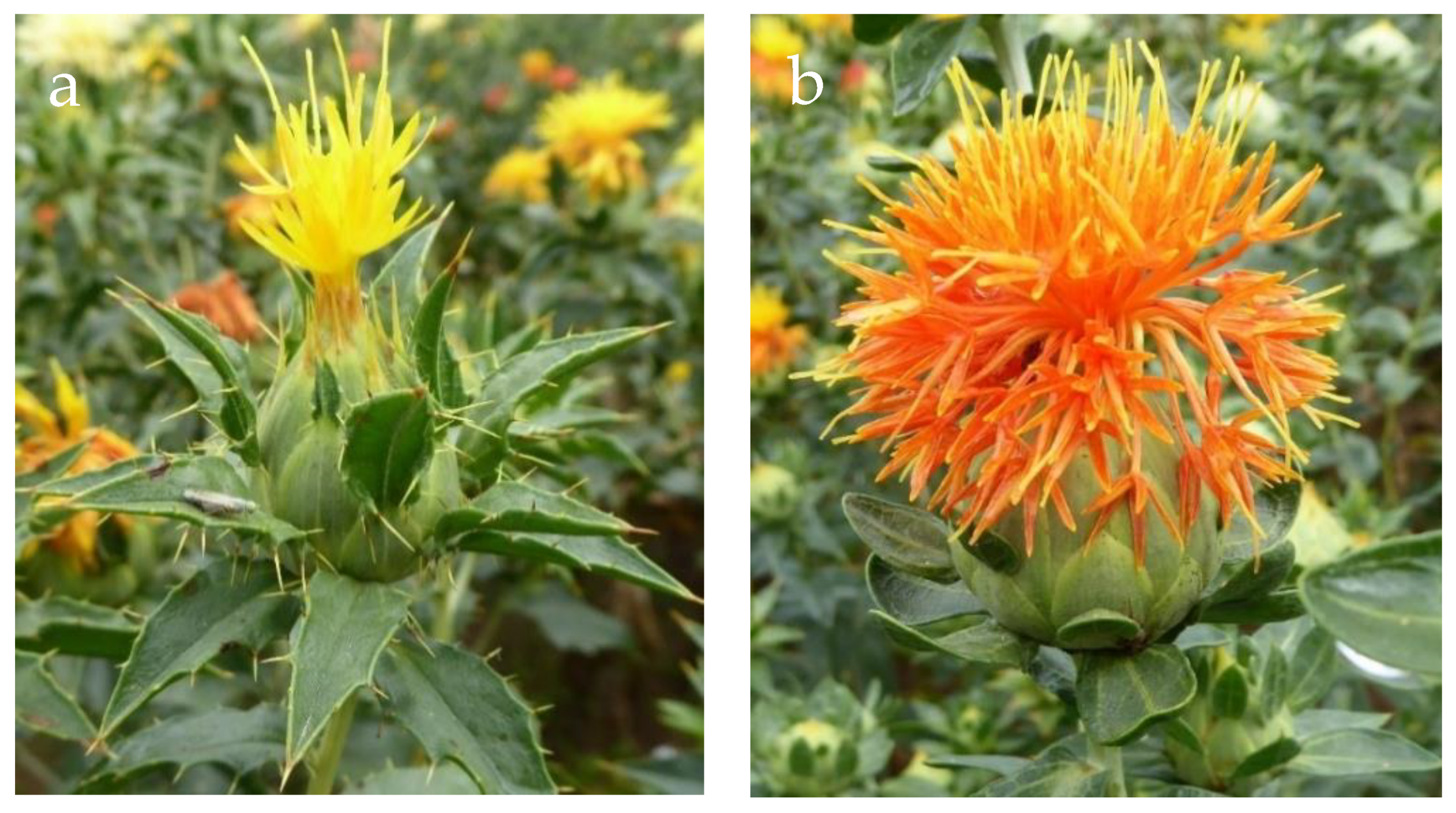
2.1. Plant Material

Two cultivars of safflower were used in this experiment. These two cultivars were selected because of their different origin (one German and one Chinese cultivar) and flower color characteristics. Both cultivars are mainly used for floret production. While the German cultivar, “C1”, is spiny with mainly yellow flowers, the Chinese cultivar, “C2”, is thornless, with mainly orange flowers (Figure 1).

2.2. Site Characteristics

The field experiments were carried out in 2017 and 2018 at the experimental station Ihinger Hof of the University of Hohenheim in southwestern Germany (48°44′ N, 8°55′ E, 478 m a.s.l). The average temperature is 9.6 °C, with an annual average rainfall of 683.4 mm. In comparison, the experimental years 2017 and 2018 had mean temperatures of 9.2 °C and 10.2 °C, and annual rainfall of 654 mm and 526 mm, respectively. The weather data was recorded by an automatic weather station close to the fields. In 2018, in almost all months (except June), the average temperature was higher than in 2017 (Table 1). In addition, maximum temperatures differed between the two years, with higher values for May and June in 2017 and for July and August in 2018. On average, rainfall was higher in 2017 compared to 2018, with most of the rainfall occurring during the flowering period (July). Solar radiation was higher in 2018 (except June) compared to 2017.
The soils were classified as vertic Luvisol in 2017 and vertic Cambisol in 2018 [29]. The soil texture was determined according to the method described by Köhn [30]. Most of the Luvisol and Cambisol soils are fertile, and are appropriate for the cultivation of many types of crops [29,31]. Inorganic mineral nitrogen contents in soil (Nmin) were measured according to the method described by Thun and Hoffmann [32], by the use of a flow injection analyzer (FIAstar 5000 Analyzer, FOSS GmbH, Hamburg, Germany). Marked differences can be seen in the mineral nitrogen content in 0–90 cm depth, which totaled around 124 and 45 kg N ha−1 in 2017 and 2018, respectively (Table 2). The organic carbon contents were determined with a vario Macro cube (Elementar Analysesysteme GmbH, Hanau, Germany) based on the method described by Dumas [33]. Organic carbon contents in the upper two soil layers were the same in both years, with 1.2% at 0–30 cm and 0.7% at 30–60 cm depth. At a depth of 60–90 cm, the organic carbon contents differed, with 0.6% in 2017 and 1.3% in 2018. In 2017, the upper two soil layers had a lower clay concentration but a higher silt concentration compared to 2018.

2.3. Field Experiments

The field trial was designed as a randomized, complete block design with three replications for a total of 24 plots in each year with a plot size of 32 m2 (8 m × 4 m). Two safflower cultivars (German (C1) and Chinese (C2)) were grown in two row spacing (12 (S1) and 33 cm (S2)) and two sowing densities (40 (D1) and 75 plants m−2 (D2)) to determine the cultivar and management effects on plant morphology, growth, and final yield. Row orientation was north–south in 2017 and east–west in 2018. The S1 plots contained 28 rows, the S2 plots 12 rows.
Before the field trial was established, previous crops were wheat and triticale in 2017 and 2018, respectively. After harvesting, the residues of those crops were incorporated with the cultivator “POM Meteor” (MEZGER Landtechnik GmbH and Co. KG, Ditzingen, Germany) to a depth of 5 cm. Five months before sowing, the fields were ploughed with a “Juwel 8 TCP V” (LEMKEN GmbH and Co. KG, Alpen, Germany) to a depth of around 25 cm. Soil samples were taken in April 2017 and 2018 to determine the mineral nitrogen content, organic carbon content, and soil texture at depths of 0–30, 30–60, and 60–90 cm (Table 2). Shortly before sowing, the seed bed was prepared by tilling with the rotary harrow “HRB 403” (Kuhn Maschinen-Vertrieb GmbH, Genthin, Germany) and the prism roller “Simplex” (Güttler GmbH, Kirchheim/Teck, Germany) to a depth of 6 cm in 2017 and 2018. Safflower was sown at a depth of 2 cm on 25 April 2017 and 19 April 2018 with a plot driller “Deppe D82” (Agrar-Markt DEPPE GmbH, Bad Lauterberg-Barbis, Germany). The target-value of soil mineral nitrogen content was 80 kg N ha−1. Based on Nmin before sowing (Table 2), in 2017, no nitrogen fertilization was required, while 40 kg N ha−1 was applied as calcium ammonium nitrate with the fertilizer broadcaster “UKS 230” (RAUCH Landmaschinenfabrik GmbH, Sinzheim, Germany) shortly after sowing in 2018. Weeding was done manually twice in 2017, 35 and 43 days after sowing (DAS). Due to the high weed pressure in 2018, weeds were manually removed eight times (6, 11, 14, 19, 22, 26, 33, and 41 DAS) until the beginning of the branching stage, at which time the plants are no longer susceptible to weeds [34,35,36].

2.4. Data Collection

2.4.1. Non-Destructive

Measurements were conducted in the center rows of the plots at a weekly interval starting at 35 DAS in 2017 and 26 DAS in 2018, when the plants had reached leaf development [34]. BBCH stage according to Flemmer et al. [34], plant height and width (perpendicular to the row orientation), number of green and senescent leaves, number of internodes and branches of main shoots, and the total number of inflorescences (capitula) were determined. At the beginning, these measurements were recorded on 10 plants per plot, which were randomly chosen in the center rows. Due to the large amount of work required, the measurements were done on only five plants per plot after the fourth sampling date.

2.4.2. Destructive

During the growing period, the biomass partitioning to different plant parts was determined at 14-day intervals until final grain harvest. The first samples were collected 55 DAS in 2017 and 39 DAS in 2018, when most plants had started branching. In the center rows of each plot, an area of 0.25 m2 was cut at the soil surface, and the fresh weight of the whole sample was recorded. Two representative plants per sample, which were equal to the average in height and weight, were selected and separated into branches, leaves, senescent leaves, capitula, and florets. The leaf area was determined with a scanner. Due to the large number of leaves, only a subsample was scanned. According to Corre-Hellou et al. [37], the total leaf area was calculated using the specific leaf area (SLA) of the subsample and the dry weight of all leaves. The fresh weight of all plant parts was determined, dried at 40 °C (florets), 70 °C (samples for subsequent nitrogen analyses), or at 100 °C until a constant weight was achieved to determine dry matter. Using the ratio of dry to fresh weight of all plant parts of the two separated plants and the remaining dry weight, the total dry weight of all plant parts of the harvested area was calculated.
In addition, plants from an area of 0.25 m2 were cut at the soil surface each week during the flowering period. The fresh weight of the whole sample was recorded and then separated into capitula, florets, and residual plant parts, and the fresh weight of these plant parts was determined. All plant parts and a subsample of residual plant parts were dried as described above, and the dry weight and dry matter concentrations were recorded. Using the ratio of the dry to fresh weight of the subsamples of residual plant parts, the dry matter of the residual plant parts of the harvested area was calculated.
Florets were harvested when most flowers bloomed on three consecutive days (97–99 DAS in 2017, 96–98 DAS in 2018), with one replication on each day. An area of 1 m2 was cut at the soil surface and the fresh weight of the complete sample was determined. The sample was separated into capitula, florets, and residual plant parts, and the number of capitula was recorded. The fresh weight of all listed plant parts was recorded, and all plant parts and a subsample of residual plant parts were dried as described above, and dry weight and dry matter concentration were calculated.
In addition to florets, a harvest of grains was performed on two consecutive days (126 and 127 DAS in 2017, 124 and 125 DAS in 2018), as soon as the plants reached maturity. In each plot, an area of 1 m2 was cut at the soil surface, and the fresh weight of the complete sample was determined. The whole sample was divided into capitula and residual plant parts. Due to the difficulty involved in separating grains from the capitula, only a subsample was divided into heads, grains, and residual plant parts. All these parts were weighed, dried until constant weight was achieved, and then weighed again to record the dry weight and dry matter concentrations of all the plant parts. The dried capitula of the whole sample were threshed with a laboratory thresher for single plants, “LD 180” (Wintersteiger AG, Ried/I., Austria), in order to obtain the grain yield of 1 m2.
The total nitrogen concentrations of the capitula, florets, grains, and the remaining plants were analyzed using a vario Macro cube (Elementar Analysesysteme GmbH, Hanau, Germany) according to the method described by Dumas [33].

2.5. Model Input

The following minimum data were used as model inputs for the model simulation: site characteristics (latitude, longitude and slope), daily weather data (global solar radiation, maximum and minimum temperature, rainfall, wind speed, and relative humidity), soil data for different depth (Table 2), initial conditions (e.g., previous crop and its residues), and management data (e.g., cultivar, sowing date, sowing density, row spacing, and tillage) [38]. The model was simulated with water balance turned on. Due to the fact that the experimental station could only take soil samples to 90 cm and safflower is a deep-rooting plant, the soil was modelled to be deeper in DSSAT [1,3]. The soil water-holding traits of the 60–90 cm layer were replicated, and three more layers to 180 cm were created.
Destructive samplings were carried out every two weeks or weekly during flowering on an area of 0.25 m2, but larger samples consisting of 1 m2 land area were collected during the main flowering and at the final grain harvest. Due to their smaller statistical variability, sample cuts of larger land areas were more trustworthy than cuts of smaller areas [27]. Therefore, it was necessary to compensate for this difference in size with a bias-adjustment [27,39]. As a reference, the 1 m2 cut at the main flowering time (fifth cut on 31 July in 2017 and sixth cut on 24 July 2018) was taken, because at this time, the plant growth had almost reached a plateau. To calculate the bias-adjustment, the tops weight of the various destructive cuts was taken. For example, in 2017, the computed land-area tops weight of the fifth (large area reference cut) cut was divided by the computed land-area tops weight of the fourth (small area) cut. The same was done in 2018. From these calculations, the mean bias value was calculated. This resulted in bias-adjustment coefficients of 0.93 for 2017 and 0.85 for 2018. In the next step, all numerical and weight-dependent variables of the smaller samples (0.25 m2) were multiplied by the year-dependent bias-adjustment coefficient to compensate for the bias associated with the lower level of precision of the smaller sample size.

2.6. Model Evaluation and Adaptation Based on Literature and Data

The default model with input weather, soils, and management information was simulated, and the simulations were compared to the observed phenology and growth dynamics. Where simulations disagreed with observations, parameters (in species, ecotype, and cultivar files) were modified in a sequential approach, as used by Boote et al. [26], in the following order: (1) reproducing the crop life cycle (phenology, e.g., time to emergence, first leaf, reproductive stages, and maturity), (2) rate of leaf appearance, canopy height, and width, (3) specific leaf area, leaf area index, and partitioning among vegetative organs, including rate of total biomass accumulation, (4) onset, rate, and duration of pod addition and seed growth, and lastly, (5) new coding to mimic floret growth. See the following sections in Results and Discussion for the parameter modifications targeted against specific crop observations. Model improvement with modified parameters was judged by improvement in the simulated means, root mean square error (RMSE), and Willmot Agreement Index (d-index; for definition of statistical indices, see Section 2.7) of the various observed plant components being targeted. While the approach was sequential, there was some iteration (stepping back to improve a previously-modified parameter). Besides modifications based on comparisons with the observed data, some parameter modifications were made based on a literature review, while some shifts in cardinal temperatures were based on the contrast between the warm versus cool weather of the two seasons. There was no automated optimization. Rather, the DSSAT graphical program computes the statistics (mean, RMSE, and d-index) of the targeted time-series observations for each of the 16 treatments (2 cultivars × 2 row spacing × 2 sowing densities × 2 seasons). By observing the graphs and statistics, we could determine the parameters that needed modification, although some iteration and sensitivity analysis was involved. For a given observation, e.g., leaf weight, we computed the average of the simulated and observed time-series means, the RMSE, and the d-index, over the 16 treatments. The goal was to come close to the observed mean, to reduce RMSE, and to increase the d-index for the important targeted observations. Final harvest values were only given the same weighting as part of the time-series data.

2.7. Statistics

The Willmott Agreement Index (d-index, (1)) and the root mean square error (RMSE, (2)) were computed to evaluate the robustness of the simulated data with the measured data, and were calculated as follows [40,41]:
d - index   =   1 [ i = 1 N ( S i     M i ) 2 i = 1 N ( | S i M ¯ | + | M i M ¯ | ) 2 ] ,   0 d 1
RMSE   =   1 N i = 1 N ( S i     M i ) 2
where N is the number of sample data points, S i are the simulated values, M i are the measured values, and M ¯ is the mean of the measured values.
The d-index is an indicator of consistency between the tendencies in simulated and measured data, and is between 0 (no fit) and 1 (perfect fit). The RMSE shows the general difference between the simulated and measured data expressed in the unit of the variable, and should be as small as possible [40,41,42,43].

3. Results and Discussion

3.1. Model Modification

Testing the existing safflower model with the data collected in a two-year field experiment indicated that major changes in the species, ecotype, and cultivar files were needed to improve model simulations [24]. By comparison to good but slight under-estimations in the year 2018 (high yields, hot year), the simulation results indicated that the model overestimated the values of 2017 (lower yields due to suboptimal wet weather conditions after the beginning of flowering). Thereafter, the model parameters were modified considering data sets from both years with different environmental conditions, using 16 data sets each (2 years over 8 treatments: 2 cultivars, 2 row spacing, and 2 sowing densities) (see Figure 5a).
The measured observations showed relatively small differences for the cultivation methods (row spacing and sowing density) (see Figure 5a). Because the response of the crop model to cultivation methods was also relatively small, we decided to focus on the main differences between cultivars and years, and therefore, only four plotted lines (two cultivars in two years) are usually shown in the following graphs. From the recorded raw data, mean values for the treatments of the respective cultivar from the respective year were calculated. However, despite the focus on the four treatments (two cultivars in two years) for the graphs in this paper, all model modification and associated statistics of model fit were based on data of all 16 treatments. In the crop model, row spacing and sowing densities were entered for each treatment.
Model parameter modification was carried out in a sequential process as described in Section 2.6; only the final simulated outputs and parameterization values are given below.

3.2. Life Cycle and Canopy Development
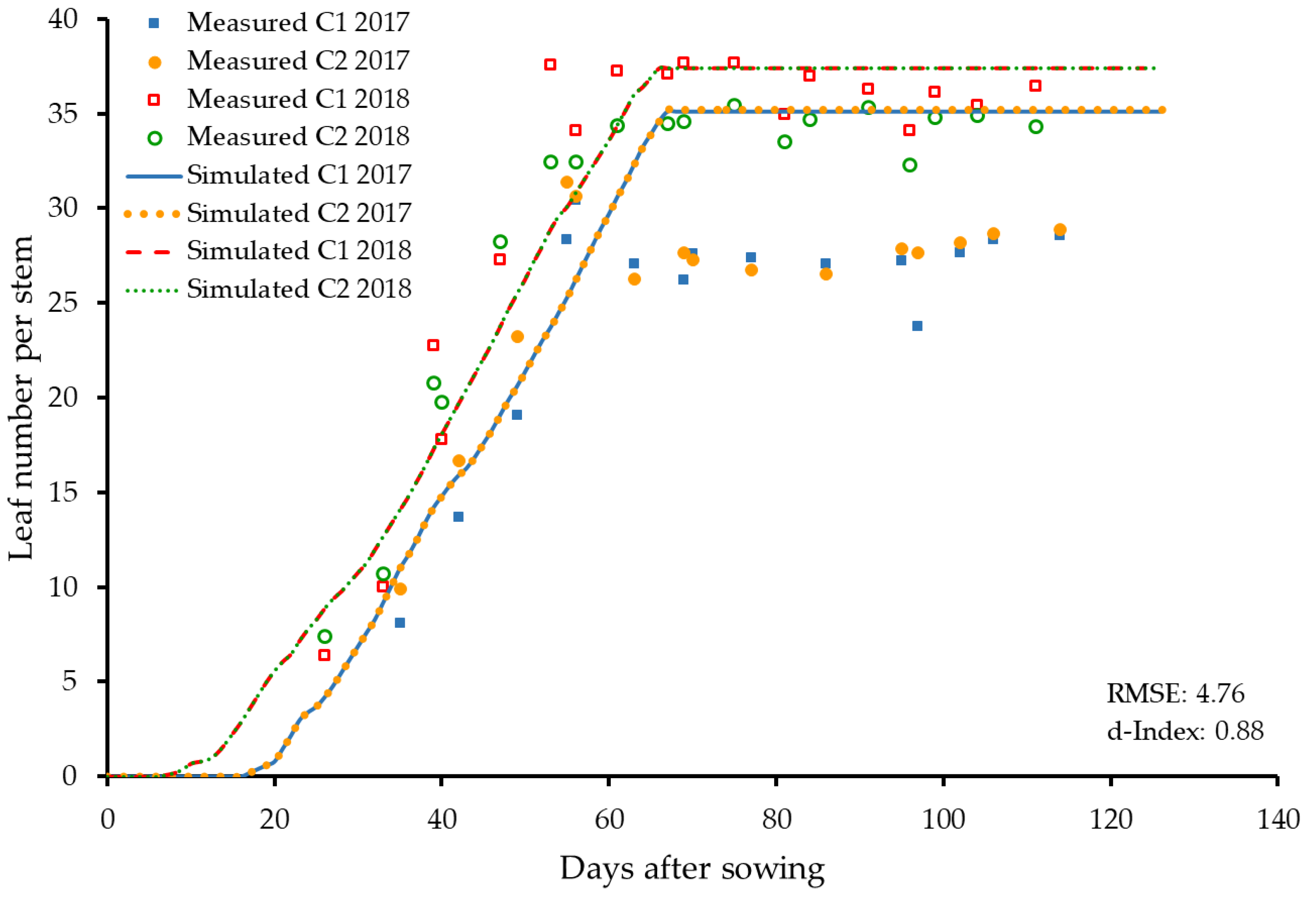
With a systematic and sequential approach to model adaptation, one of the first tasks should be to properly simulate plant development and life cycle [44]. An essential part of the CROPGRO Crop Template is the phenology simulation which uses parameters of the species, cultivar, and ecotype files, which include, for example, information about the cardinal temperatures in the species file or phase durations for different life cycles in the cultivar file [23]. Because plant development, life cycle, and plant growth are influenced by temperature and day length, the correct cardinal temperatures and the different physiological durations are an important first approach [23,45,46].
Therefore, the first step was to evaluate the cardinal temperatures in the species file and the different durations for the respective development phases in the cultivar and ecotype files (Table 3).
The defined cardinal temperatures include the base temperature (Tb), the first optimum temperature (Topt1), the second optimum temperature (Topt2), and the maximum temperature (Tmax) in °C (Table 3). For the phenological parameters, it was necessary to set a lower Topt1 temperature for the rate of leaf appearance. The measured leaf appearance data were used to adjust the value for the Topt1 in the model from the default 28 °C (based on [47]) to the modified 22 °C. Based on the measured data, the resulting vegetative growth curves and literature references indicated that safflower can tolerate and grow well at lower temperatures during vegetative and reproductive phases [2,48,49]. Another important modification was related to the temperature effects on leaf photosynthesis. Initially, the cardinal temperatures of sunflower and soybean photosynthesis were used [44,50,51]. Based on the measured data of our two-year German field experiment, the temperatures were shifted towards those used in the fababean model, thereby achieving an overall better fit. This change is supported by the literature, suggesting that safflower can tolerate temperatures down to −7 °C, depending on the stage of development [26,44,52].
Further, physiological day durations are an essential model component [23,45]. Table 4 and Table 5 show the phase duration changes made in the ecotype and cultivar files. The model was adapted to the two cultivars used in the field trials in 2017 and 2018. After the modifications of the species, ecotype and cultivar files were completed, Singh’s original data of the cultivar “PI8311” was evaluated with the new model settings (Table 4 and Table 5). The modified version of the model resulted in a better fit for Singh’s experiments [27], indicated by statistical parameters Wilmott Agreement Index (d-index) and RMSE [40,41].
Safflower is generally regarded as a daylength-neutral, long-day plant, and the origin of the cultivar plays a decisive role [3,53]. In order to be able to correctly model the growth phases, such as the time to anthesis, safflower is defined here as day-neutral in the model [27], setting critical long daylength to 23.0 h and PPSEN = 0.001. Because of the definition as a day-neutral plant, the minimum rate of reproductive development under long days and optimal temperatures is irrelevant, and therefore, is not listed in the cultivar file table (Table 5).
In the following section, important parameters are described in more detail. All modifications made in the model are listed in Table 3, Table 4, Table 5, Table 6, Table 7 and Table 8.

3.2.1. Leaf Number

In order to design the crop life cycle correctly, it is very important to calibrate the plant growth parameters in the species file correctly, which includes the effect of temperature on leaf appearance rate, leaf relative expansion, and other processes (Table 3) [45]. Based on the measured data, the first optimum temperature (Topt1) for the leaf appearance rate was reduced from 28.0 to 22.0 °C. Depending on the stage of development, safflower has different temperature requirements [48]. Since leaves are also formed during the rosette stage, and safflower tolerates very low temperatures during this stage, the lower temperatures can be justified [3,49,52]. The parameters affecting leaf appearance rate could not be calibrated for the original model of Singh et al. [27] because the leaf number was not recorded in their experiment. Given the lack of data, default parameters were assumed from the soybean model; this may explain the need for modifications in the present work [44]. It was important to set the leaf appearance rate correctly. The time between planting and emergence (PL-EM) was too short, and was increased to 5.0 for both the PI8311 cultivar and the new cultivars (Table 4). The model is designed to simulate the appearance of fully developed leaves. Because leaf tips were counted during this data collection for both non-destructive and destructive measurements, the time between emergence to first true leaf (EM-V1) had to be shortened by half. In addition, the rate of leaf appearance (TRIFOL) was increased significantly from 0.36 to 1.00, based on the observed rate of leaf appearance over time (Figure 2 and Table 4).
This was an essential step, because the rate of V-stage progression (given as leaf number on the main stem) affects the modeled shift in the partitioning of daily assimilates among leaf and stem and the leaf area index (LAI) as well. The maximum leaf photosynthetic rate at 30 °C, 350 ppm CO2, and high light (LFMAX) was adjusted based on the correct prediction of biomass over time, and was set at 1.50 mg CO2 m−2 s−1 for the PI8311 cultivar, 1.55 mg CO2 m−2 s−1 for the German, and 1.80 mg CO2 m−2 s−1 for Chinese cultivar (Table 5).
The simulated and measured leaf number on the main stem for both cultivars in both years is shown in Figure 2. Comparing the simulated and measured leaf number on the main stem, the year 2018 could be simulated very well, but 2017 was overpredicted, at least after the 50th DAS. This was also reflected in the RMSE and d-index separately for both years. In 2017, the RMSE was 6.52, the d-index 0.77, while 2018 had a lower RMSE of 3.01 and a higher d-index of 0.97. A possible reason for the good plant growth in 2018 could be the warm and dry weather during flowering, which is very suitable for safflower because sunny, warm conditions accelerate growth, and moisture could promote diseases (Table 1) [2,54,55]. A comparison between the simulated and measured leaf number of the main stem of both cultivars and years resulted in a RMSE of 4.76 and a d-index of 0.88 (Figure 2).

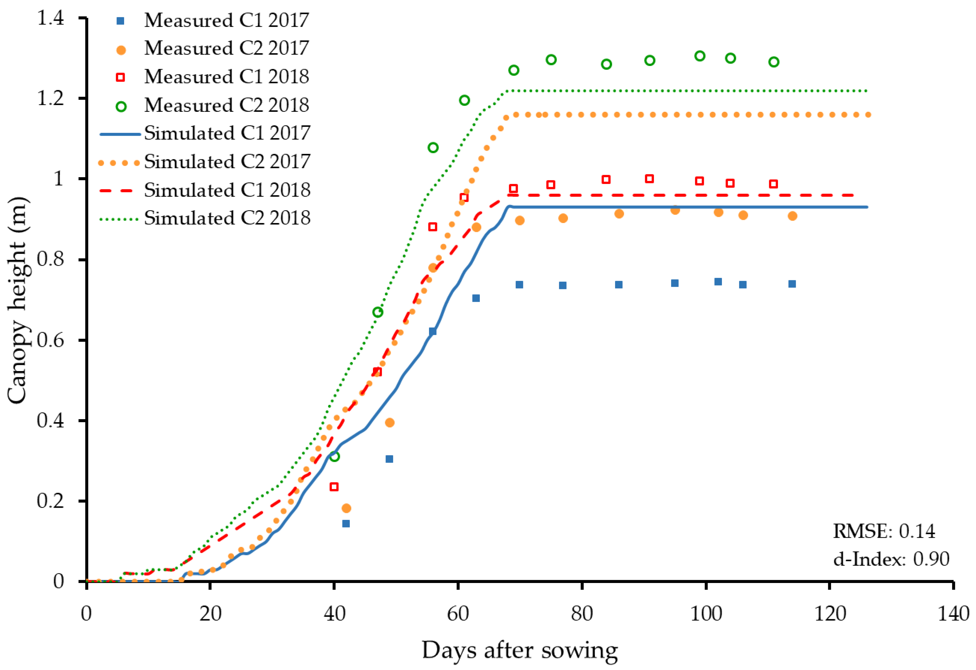
3.2.2. Height and Width

The height and width of the plants were measured weekly. Parameters for both the “PI8311” cultivar and the newly-added two cultivars “C1” and “C2” were modified (Table 4). The relative width in comparison to the standard width per internode (RWDTH) was modified for the PI8311 cultivar from 0.85 to 0.75 and for the new cultivars “C1” and “C2” to 0.75 and to 1.00 (Table 4). Also, the canopy width increment (YVSWH) and internode length (YVSHT) as a function of plant vegetative node stage had to be modified (Table 7). A comparison between the simulated and measured canopy widths for all four treatments showed an underprediction of canopy width with a RMSE of 0.08 and a d-index of 0.66 (data not shown). The relative height parameter (RHGHT) that modifies the standard internode length per internode was changed for the PI8311 cultivar from 0.85 to 0.75 and for the newly-added cultivars “C1” and “C2” to 0.80 and to 1.00 (Table 4). There was an impact of year on canopy height (Figure 3). The canopy height in 2017 was overpredicted with a RMSE of 0.20 and a d-index of 0.83, but 2018 was simulated very well, with a RMSE of 0.07 and a d-index of 0.98. The reasons for this could be the temperature, which affects the plant height [48,56,57]. Figure 3 shows that plants in 2018 were taller than in 2017, which could be related to the warmer and drier weather conditions in 2018 (Table 1). Additionally, in both years, the Chinese cultivar (C2) grew taller than the German one (C1) (Figure 3); a possible reason for this could be that the cultivar or its origin also plays an important role in how tall the plants grow [48,56,58]. Knowles [58] characterized many safflower cultivars, and showed that the Far Eastern cultivars grow taller, whereas the European ones tend to be medium-sized. After modifying the parameters based on the obtained dataset, the canopy height had a RMSE of 0.14 and a d-index of 0.90.

3.2.3. Time to Flowering

To model the growth of safflower, it is important to notice that the capitula (flower heads) are already present before flowering occurs, and that the seeds begin to grow shortly after flowering [27]. In order to represent this correctly in the model, the true anthesis is ignored, and the time of the first capitulum is entered as first pod date (PD1T). Hence, the time (in photothermal days, PD) between the “false” first flower and the first pod (capitulum) (FL-SH) was defined. The sum of the time from plant emergence to flower appearance (EM-FL), plus the time between the first flower and first seed (FL-SD), is entered to achieve “true” anthesis [27]. With the correct phase duration between first flower and first seed (FL-SD) and the correct first seed date (PDFT), as well as the time span between first seed and physiological maturity (SD-PM), the correct physiological maturity is achieved. In addition, the cardinal temperatures of vegetative growth were modified prior to this step in order to allow more rapid plant growth at lower temperatures to simulate vegetative growth correctly (Table 3). The time between plant emergence and flower appearance (EM-FL) was shortened, and the time between first flower and first pod (FL-SH) had to be extended (Table 5). Nevertheless, it was important to keep the time between EM-FL as long as possible and the time between FL-SH as short as possible in order to achieve a better transition of partitioning between leaf and stem. After flowering and the time of the first pod was set correctly, the time from first flower to the appearance of the last leaf on the main stem (FL-VS) could be modified. FL-VS affects the timing of the last leaf appearance as well as the endpoint of any further height increase, and was extended from 7.0 to 14.0 PD (Table 4) [34].

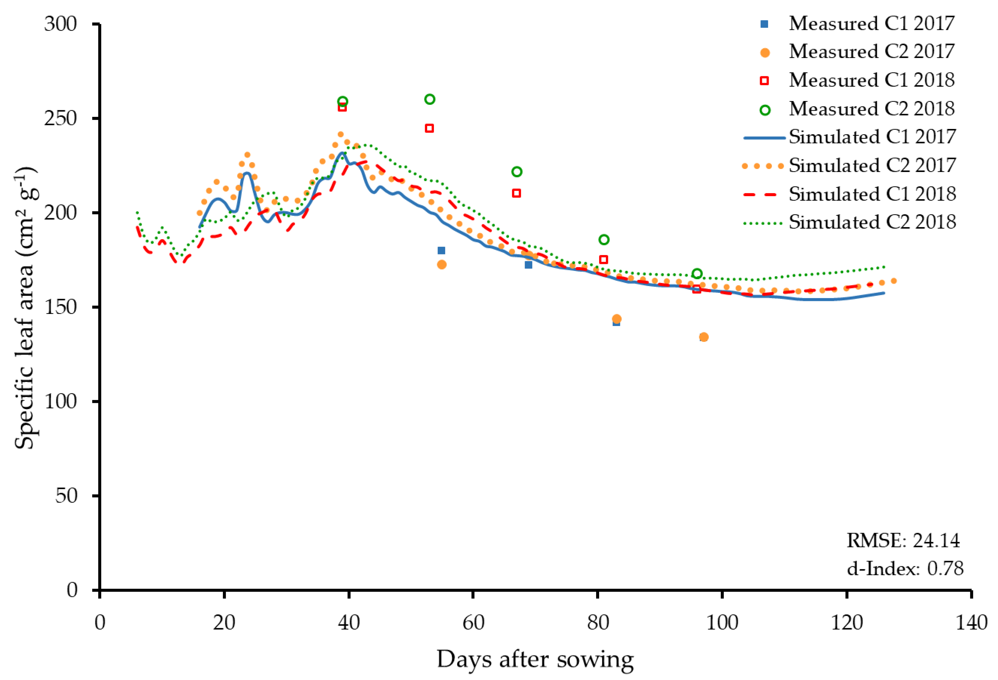
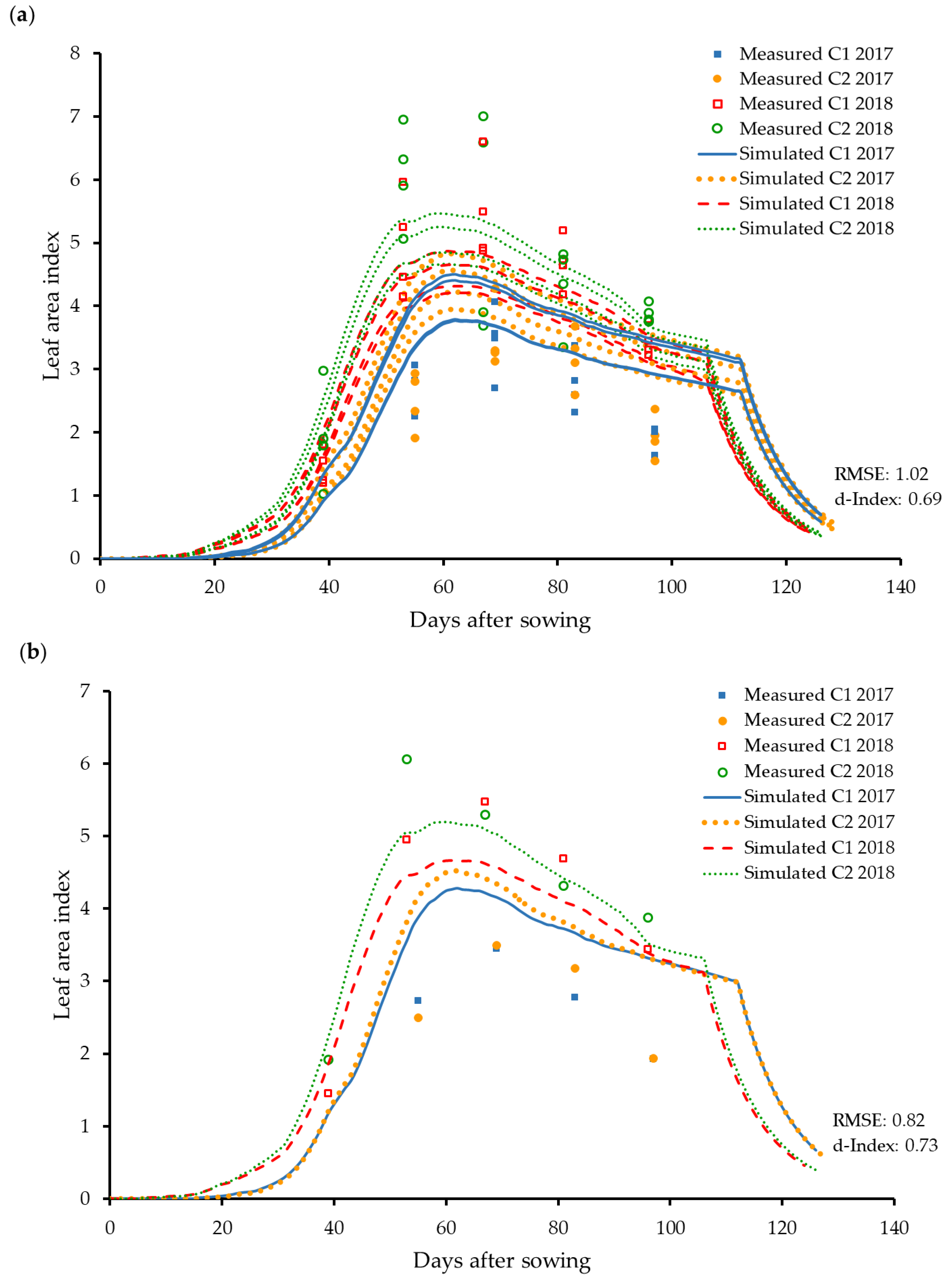
3.2.4. Specific Leaf Area and Leaf Area Index

In the default model, important parameters affecting the SLA were assumed to be similar to the soybean model. The model coding allows SLA to be influenced by solar radiation and cardinal temperatures; therefore, it was necessary to adapt the original model parameters affecting SLA to new environmental conditions in Europe and to the two different cultivars (Table 3) [24,59]. Simulated LAI indicated that leaf expansion started too slowly, and that SLA was too low; therefore the SLA-related parameters (especially SLAMIN) were increased. Based on the measured data, the base temperature (Tb) for leaf expansion was reduced from 12.0 to 8.0 °C and the first optimum temperature (Topt1) from 22.0 to 21.0 °C. The lower Tb and Topt1 for leaf expansion also acted to increase SLA and LAI.
As the SLA of a cultivar under standard growth conditions (SLAVR) and the specific area of the standard reference cultivar at the peak early vegetative phase (SLAREF) should be close to the same value, the SLAVR for the cultivars “PI8311” and “C1” were set to 250 cm2 g−1, and for the cultivar “C2” to 260 cm2 g−1 (Table 5). In the species file, the value SLAREF was set to 260 cm2 g−1 (Table 6). Closely linked to these values are the upper and the lower limits of SLA with regard to the response to solar radiation (SLAMIN, SLAMAX). The increase in SLAMIN from 110 to 260 cm2 g−1 had the largest effect on SLA, while SLAVR and SLAREF were set to 260 cm2 g−1 to be close to SLAMIN (Table 6). Modification of SLAMAX was not necessary.
All these modifications resulted in significant improvements in the simulated SLA by increasing the d-index and reducing the RMSE. After all the modifications were carried out, a comparison of the simulated and the measured data showed an underprediction of the values of 2018, with a RMSE of 27.46 and a d-index of 0.83, and an overprediction of the values of 2017, with a RMSE of 20.83 and a d-index of 0.72. Comparing the simulated and measured SLA of all treatments over both years and both cultivars, a RMSE of 24.14 and a d-index of 0.78 was obtained (Figure 4).
All the modified parameters related to SLA led to an improvement of LAI in both the RMSE and the d-index. Figure 5 shows the LAI. Figure 5a shows simulations of all 16 treatments, while Figure 5b has only four curves (two cultivars in two years), and neglects the small effects of row spacing and sowing density.
The correct termination of leaf area expansion and the correct peak of LAI was achieved by reducing the time between first flower and end of leaf expansion (FL-LF) from 20.25 to 18.00 PD (Table 5). In Figure 5, the slow decline of the simulated LAI at the end of life cycle is a result of protein mobilization and the value of SENRTE (Table 6). The following steep decline is set by maturity (SD-PM) and the SENRT2 (Table 6). This has already been noted by Stern and Beech [60], who reported a rapid rise in LAI to 4–5, and then a drop to almost zero at harvest.
After modification, simulated LAI for 2017 was overpredicted compared to the measured LAI, with a RMSE of 1.12 and a d-index of 0.51 (Figure 5b). In 2018, the opposite was observed, where the simulated values slightly underestimated the measured values for LAI, with a RMSE of 0.53 and a d-index of 0.95. One reason for the higher LAI in 2018 could be the warm and dry weather conditions, which are very appropriate for safflower growth [2,54]. The adjustment of the parameters to best simulate both years and both cultivars resulted in a RMSE of 0.82 with a d-index of 0.73.

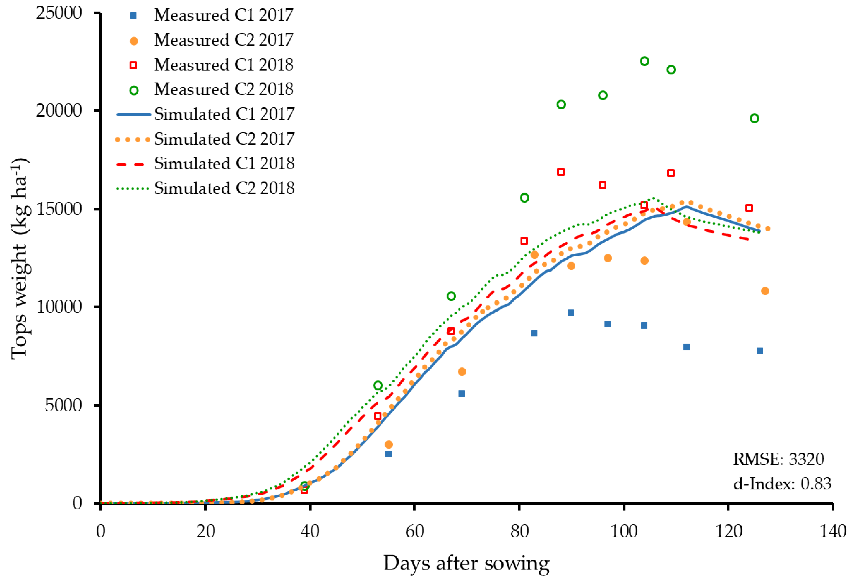
3.3. Dry Matter Accumulation and Partitioning

The dry matter growth of new plant organs depends on various factors, such as the availability of carbohydrates and the partitioning to different plant parts [23]. Important parameters influencing photosynthesis and dry matter accumulation include the partitioning to the root. If considerable assimilates are allocated to the root very early in the growth cycle, this occurs at the expense of shoot growth and leaf area formation, which then develop more slowly [45]. Because partitioning depends on the growth stages of the plant, the following table shows the partitioning-fractions, internode length, and leaf senescence in relation to the respective V-stage (Table 7) [23].
The partitioning functions are used to determine the daily distribution of assimilates to tissues at a given V-stage. It is important to distribute this correctly, as distribution to leaf tissues defines the LAI. LAI, in turn, affects the amount of assimilates for the formation of reproductive organs during the reproductive phase. Based on the measured data, the partitioning for leaf and stem was changed, and more assimilates were shifted into the leaves. Due to the faster rate of leaf appearance based on the observed leaf number (Figure 2), the shift of the partitioning towards the stem was initially too fast (in the default model), with increasing V-stage leading to less leaf and more stem mass in the end. As the leaf appearance rate on the main stem (TRIFL) was very high, the corresponding V-stages had to be renumbered and extended (Table 4 and Table 7). Since total partitioning altogether sums up to 100%, the missing part in the partitioning after YLEAF and YSTEM always represents the partitioning to the roots. Since roots were neither harvested nor weighed in the field trials, this proportion of roots could not be evaluated. Since it was desirable that more of the partitioning go into the leaves, the fraction to stem was reduced while keeping the allocation to root unchanged, in order to retain the same total (Table 7). Another important change was the fraction of the vegetative dry matter growth allocated to leaf and stem at the end (FRLFF and FRSTMF) by decreasing the leaf and increasing the stem percentage. After the partitioning to the leaves was correctly defined as a function of V-stages, LAI was increased, allowing more photosynthesis to take place, which, in turn, increased biomass formation and, later, also reproductive organ formation. Despite these changes, the overall biomass formation was still a little too low, and SWREF (specific weight at which LFMAX is defined) was reduced to achieve a greater slope to increase the amount of biomass (Table 6).
After all the modifications had been made, the model indicated a good fit for leaf weight and stem weight, with RMSE of 327 and 1449 and d-indices of 0.78 and 0.81, respectively (data not shown).
Figure 6 shows the development of the aboveground biomass (tops) during the vegetative period. The model indicated a good fit at the beginning when the weather conditions were still relatively warm and dry (Table 1 and Figure 6). After 80 DAS, data of year 2017 were overpredicted with a RMSE of 3208 and a d-index of 0.75, whereas the year 2018 was underpredicted, with a RMSE of 3432 and a d-index of 0.91. The over- and under- predictions are mainly the result of forcing the model to best simulate the data across two different years, with 2018 being an ideal year for safflower growth, while the humid conditions in 2017 led to diseases and an overall lower yield. Comparing the simulated and measured tops weights of both years and cultivars, a RMSE of 3320 and a d-index of 0.83 were obtained (Figure 6). The decrease of the biomass after peak vegetative growth and towards 110–120 DAS is typical for safflower, and can be explained by the seed formation, leaf senescence, and maturity of the plant [60].
Because the default safflower model was adapted from the soybean model, it is possible to orientate oneself on the structures of the soybean model, in which the plant consists of roots, leaf, stem, shell, and seed [27,44,61]. These vegetative organs are defined as having constant compositions, i.e., proportions of compounds for the different organs, except that protein (N) is allowed to vary under N-stress [61]. Based on this fact, the sum of lipids (PLIPLF), protein (PROLFI), carbohydrates (PCARLF), lignin (PLIGLF), minerals (PMINLF), and organic acid (POALF) for a particular new plant organ under non-limiting nitrogen should always sum to 1.00 (Table 8) [27]. Under N stress, the actual protein can be less than the potential (PROLFI), in which case the PCARLF increases as the complement. In Table 8, only protein and carbohydrate-cellulose concentrations are shown, because other compositions of components such as lipids were not changed from the default model. Based on the nitrogen concentration data of leaves (data not shown), the target PROLFI was reduced. Since the sum of the individual components of a plant organ must always be equal to 1.00, the protein concentration was reduced from 0.356 to 0.306, while the proportion of carbohydrate–cellulose in the leaf was increased by the same amount, from 0.405 to 0.455.

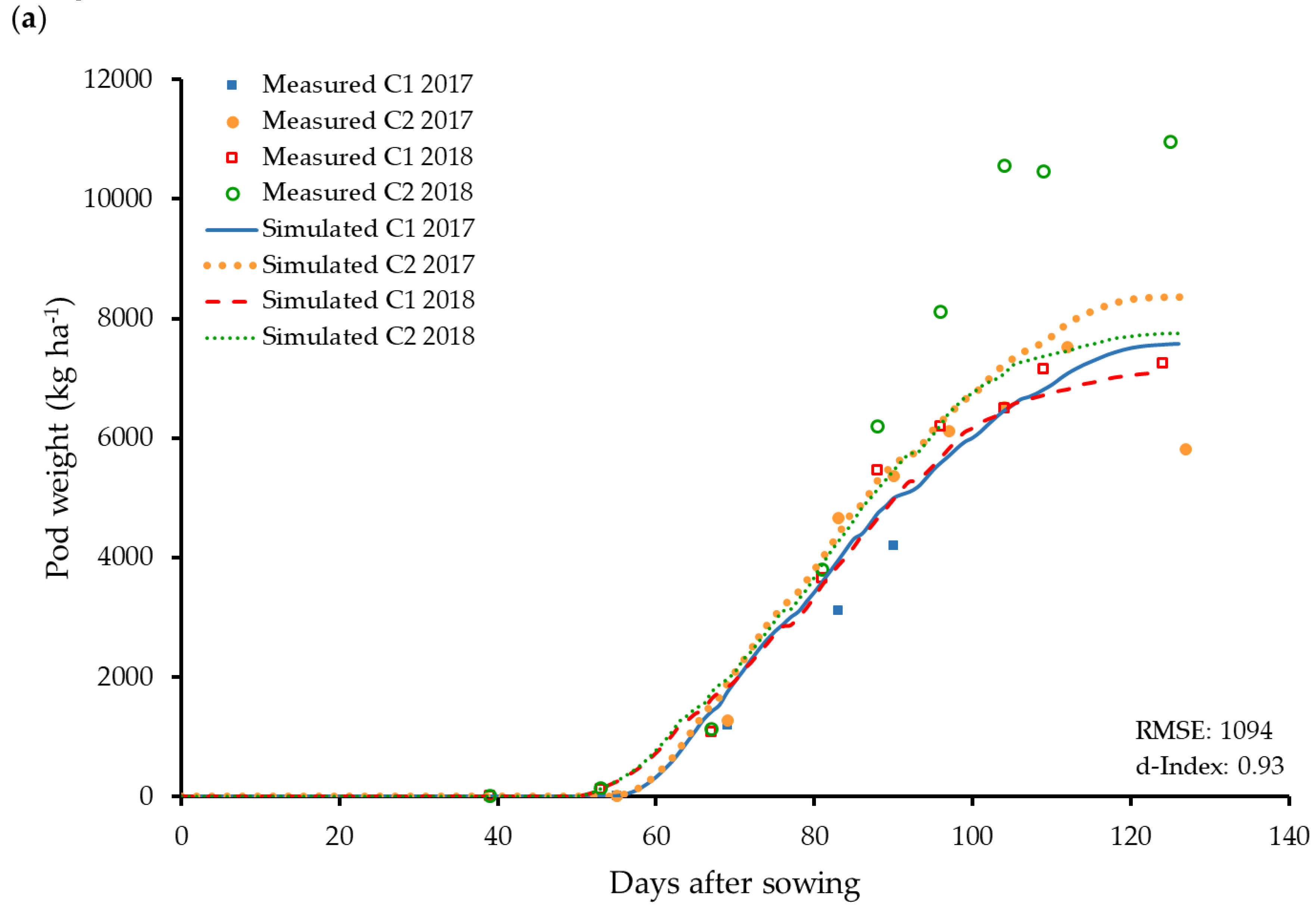
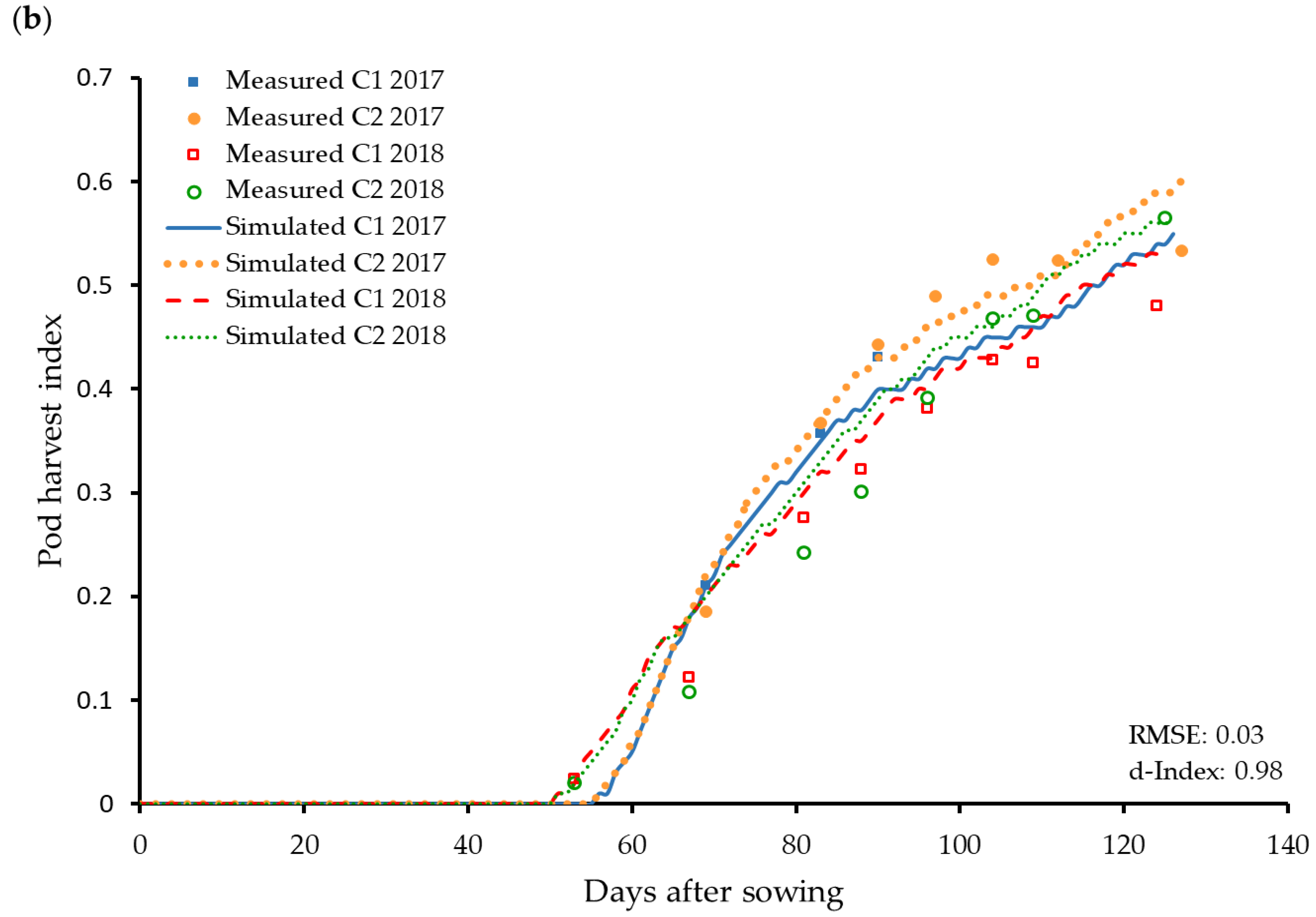
3.4. Reproductive Organs and Yield Influencing Parameters

Cardinal temperatures in the species file were changed for the pod addition rate (Table 3). In the original model by Singh et al. [27], the cardinal temperatures of the pod addition rate of soybean were used [44]. A reduction of Tb was necessary to achieve sufficiently high pod addition rate at the relatively cool temperatures observed in Germany, as compared to those in New Mexico (Table 3). Temperature for Tb was reduced from 14.0 to 9.0 °C, which also resembles the Tb of sunflower seed-set, which is 7.5 °C (Table 3) [44].
In order to set the correct onset of increase of pod dry weight and also later onset of seed dry weight, FL-SH was set to 4.5 PD, while FL-SD was set to 13.0 PD [45]. As the duration of the flowering period is influenced by genetics as well as environmental conditions such as temperature, an adaptation of the model for other cultivars was necessary [62,63]. The duration of pod addition (PODUR) also has an impact on the increase in pod and seed mass at the beginning of their formation [45]. PODUR for the default cultivar “PI8311” and for the cultivar “C1” was increased slightly, from 17.0 to 18.0 and 19.0 PD, respectively, to add pods and seeds more slowly [45]. For the cultivar “C2”, a value of 17.0 PD was used to shorten the lag phase and to add pods and seeds more rapidly (Table 5) [45]. The model code allows for indeterminate species by reserving some assimilates available for leaves and stem, even after pod and seed formation. While this maximum fraction of daily growth partitioned to seed and shell (XFRT) can be 1.0 for totally determinate plants, it is lower than that for safflower. With an XFRT value of 0.55 for the original model, not enough seeds were formed. Therefore, XFRT was increased for both the PI8311 cultivar and the two new cultivars (Table 5). By comparison, the XFRT of highly-bred soybean is 1.00 [44]. All these modifications had positive effects on the modelling of the pod weight and pod harvest index, as the RMSE was reduced for both simulated variables and the d-index was increased.
A comparison between the simulated and measured pod weights showed a slight overprediction in 2017, with a RMSE of 901 and a d-index of 0.93. In contrast, a comparison of the simulated and measured values for 2018 showed a slight underprediction, with a RMSE of 1287 and a d-index of 0.95. After the parameters were modified with data from both years and both cultivars, the comparison of the simulated and measured pod weight resulted in a RMSE of 1094 and a d-index of 0.94 (Figure 7a).
Simulated pod harvest indices for 2017 and 2018 were similar to the measured values, with RMSE of 0.026 and 0.039 and d-indices of 0.98 and 0.99, respectively. Measured pod harvest index with data from both years and both cultivars was well simulated by the model, with a RMSE of 0.03 and a d-index of 0.98 (Figure 7b).
The time between first seed and physiological maturity (SD-PM), maximum weight per seed (WTPSD), seed filling duration for pod cohort (SFDUR), and weight percentage of seeds in pods (THRSH) in the model were set on the basis of the measured data set. To define the beginning of seed maturity and physiological maturity correctly, time between first seed and physiological maturity (SD-PM) had to be extended for the cultivar “PI8311”, while the SD-PM for the other two cultivars had to be shortened (Table 5). Because genetic potential weight per seed (WTPSD) was too small for the PI8311 cultivar, the final seed size was too low, and WTPSD was increased for the PI8311 cultivar and for the two newly-added cultivars (Table 5). Because single seed growth rate depends on the maximum shelling percentage of cohorts, the shelling percentage should be a little below the measured one [45]. As a result, the weight percentage of seeds in pods (THRESH) for cultivar “PI8311” had to be reduced and THRESH for cultivars “C1” and “C2” had to be raised to 55.0 and 61.0% (Table 5). Due to the lack of measurements of seed size over time, the seed filling duration for pod cohort (SFDUR) could not simply be set. Because the simulated shelling percentage of the new dataset was a little high, SFDUR was increased from 29.0 to 30.0 PD (Table 5) [45].
Because the grain yield was only recorded at maturity, a statement about the d-index for grain yield is not possible. A comparison between the simulated and measured harvest indexes, shelling percentages, grain weights, and unit grain weights indicated a small underprediction, with RMSE of 0.06, 9.53, 1715, and 6.27, respectively, over all treatments, cultivars, and years.

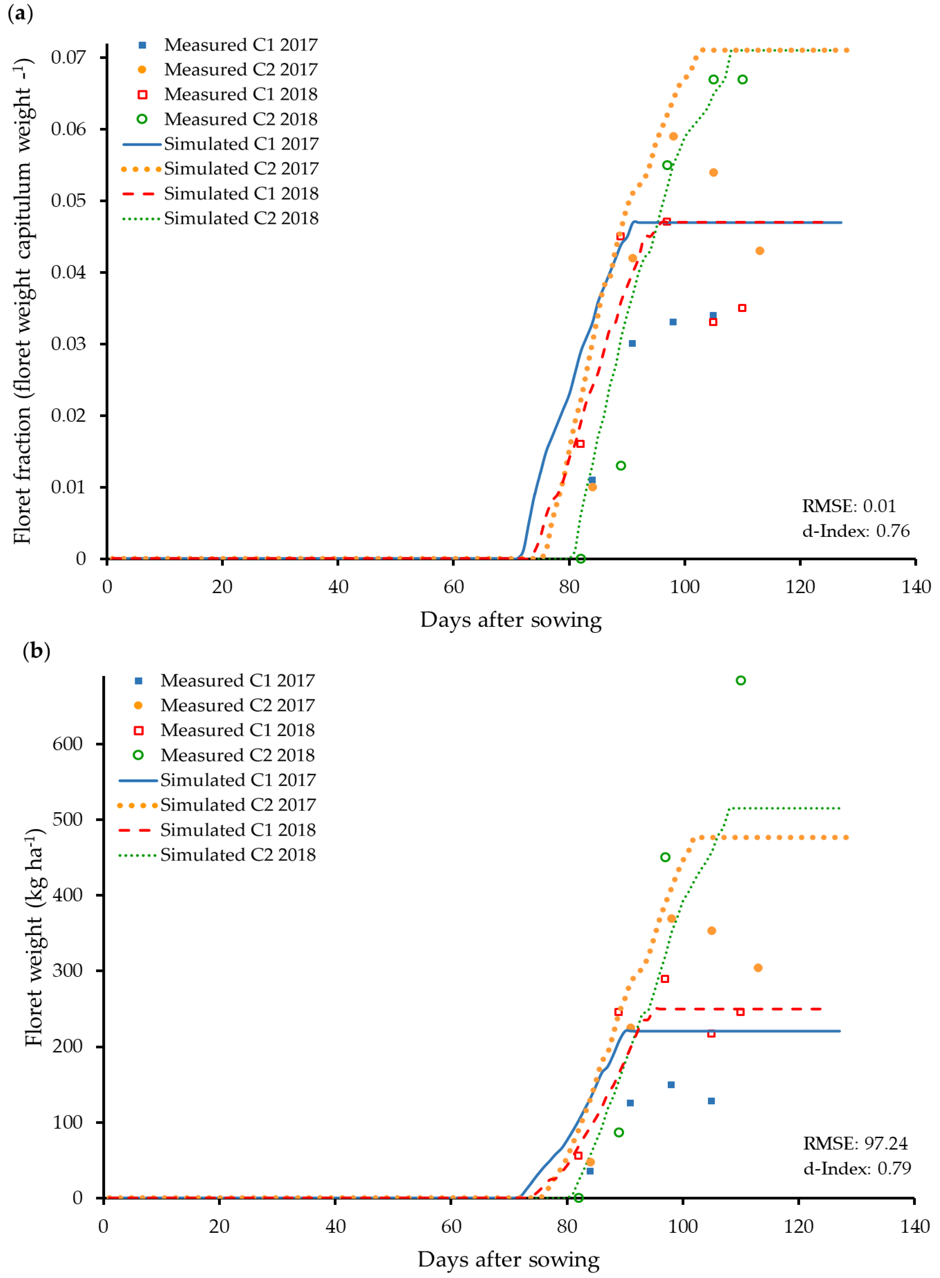
3.5. Modelling of Floret Yield and the Relationship to the Flower Capitulum

After the modification of parameters affecting pod and seed growth, a modeling approach was developed to predict the yield of the florets. In order to estimate the size, and thus, possibly the productivity of the flower pod (capitula), the ratio of floret weight to capitulum weight was calculated. The derived relationship indicated a stable but slowly-increasing ratio over time, reaching a peak ratio at the time when the highest floret yield was achieved (Figure 8a). A distinction had to be made between the two cultivars due to the different size of capitula and the mass of florets per capitulum. The developed relationship of floret fraction over time (Figure 8a) has an analogy in the model to the pod harvest index over time. A linear relationship was obtained for the ratio of floret yield to capitulum versus the pod harvest index for each cultivar. The equation of the linear relation was normalized and recorded on the basis of the maximum ratio of floret weight to capitulum weight. To predict the floret weight ratio, the values of the initial (HIPIN) and maximum (HIPMX) pod harvest index defining the onset and maximum of the floret fraction relative to the pod harvest index, the ratio of floret weight to capitulum weight (PETALX) were used for each cultivar.
Based on the lowest possible RMSE and highest possible d-index, the parameters were set to HIPIN = 0.2320 and 0.2970, HIPMX = 0.3950, and 0.4800, and PETALX = 0.04690 and 0.07080 for cultivar C1 and C2, respectively.
These parameters were used in the following Equation (3) and the result used according to Equation (4):
FPETAL = PETALX × MIN(1.0,MAX(0.0,(HIP − HIPIN)) / (HIPMX − HIPIN)))
IF (FPETAL.LT. PETALX) PETAL = PODWT × FPETAL
where FPETAL is the floret weight ratio, PETALX is the maximum ratio of floret weight to capitulum weight, HIP is the pod harvest index, HIPIN is the initial pod harvest index at which floret begins, HIPMX is the maximum pod harvest index at which floret dry matter increase ceases, and PODWT is capitulum (pod-plus-seed) weight.
The fraction of florets to pod weight averaged over four treatments of two cultivars and two years were slight overpredicted by the model, with a RMSE of 0.01 and a d-index of 0.76 (Figure 8a).
Figure 8b indicates the floret weight of the two cultivars in both years after the adaptation process. In general, cultivar C1 had a lower RMSE, i.e., 66.49, compared to that of cultivar C2, i.e., 128. However, cultivar C2 had a higher d-index, 0.87, compared to that of cultivar C1, i.e., 0.71. The reasons for the higher RMSE despite the higher, and therefore, better d-index of cultivar C2 are the generally higher floret yields of cultivar C2, which explain the higher RMSE. Floret weights in 2018 could be predicted better, with a RMSE of 96.33 and a d-index of 0.91, in comparison to 2017, with a RMSE of 98.15 and a d-index of 0.67. The better weather conditions in 2018 resulted in higher and more stable yields. A comparison between simulated and measured floret weights over both cultivars and both years showed an overprediction, with a RMSE of 97.24 and a d-index of 0.79 (Figure 8b).

4. Conclusions

A successful simulation of growth, yield, and floret yield of two safflower cultivars under field conditions in southwestern Germany with a modified DSSAT CROPGRO safflower model was achieved in this study. Model parameters were modified using field data of two cultivars grown in Germany in two years. Importantly, the model with new parameters continued to simulate well the original safflower experiments in the DSSAT, on which the prior default model parameters had been set. The newly-modified species, ecotype, and cultivar parameter files should be included in the next DSSAT model release for safflower. The introduction of the new variables PETALX, HIPIN, and HIPMX into the model made it possible to predict the floret yield at different harvest times over the flowering time separately for two cultivars.
However, further research is needed to validate the modified model, and above all, the new tool for predicting the floret yield. The performance of the model to predict floret yield should be tested with other independent data, because it has worked well under good weather conditions so far (2018), but only fairly under suboptimal conditions (2017, rain during flowering). The differentiation of the model between the cultivation systems (sowing density and row spacing) and cultivars should be further evaluated with additional experiments, as the number of branches and, thereby, also the number of capitula are influenced by plant spacing [3,64,65,66]. Water balance was turned on and a light water stress occurred in 2018, three weeks prior to physiological maturity, which could have reduced the final biomass and pod mass in 2018. Therefore, further evaluation under water deficit situations would be appropriate. The N balance was not simulated because of the low number of data values of tissue nitrogen concentration, lack of nitrogen treatments in the field trials, insecurity associated with soil N mineralization, and because the default safflower model had been simulated with N balance turned off [27]. In future studies, attention should be paid to the N balance, and the model should be tested with N fertility treatments, including zero N treatments, as well as careful initial conditions and soil N measurements. Emphasis should be placed in future experiments on recording the number of seeds, seed weight, and the development of seeds in general, to be able to improve this part of the model even further.

Author Contributions

Conceptualization, K.S., K.J.B., S.M. and S.G.-H.; methodology, K.S., K.J.B., S.M. and S.G.-H.; software, K.S. and K.J.B.; validation, K.S. and K.J.B.; formal analysis, K.S.; investigation, K.S.; resources, K.S. and S.G.-H.; data curation, K.S.; writing—original draft preparation, K.S.; writing—review and editing, K.S., K.J.B., S.M. and S.G-H.; visualization, K.S.; supervision, S.G.-H., K.J.B. and S.M.; project administration, S.G.-H.; funding acquisition, S.G.-H. All authors have read and agreed to the published version of the manuscript.

Funding

This research was funded by the German Federal Ministry for Economic Affairs and Energy within the Central Innovation Program for SMEs, grant number 16KN050530.

Acknowledgments

The authors would like to thank the technical staff of the Experimental Station Ihinger Hof of the University of Hohenheim for the agronomic management of the field trials, manpower and the possibility to use the devices.

Conflicts of Interest

The authors declare no conflict of interest. The funders had no role in the design of the study; in the collection, analyses, or interpretation of data; in the writing of the manuscript, or in the decision to publish the results.

References

  1. Emongor, V. Safflower (Carthamus tinctorius L.) the underutilized and neglected crop: A review. Asian J. Plant Sci. 2010, 9, 299–306. [Google Scholar] [CrossRef] [Green Version]
  2. Weiss, E.A. Oilseed Crops, 2nd ed.; Blackwell Science: Oxford, UK, 2000; ISBN 0632052597. [Google Scholar]
  3. Dajue, L.; Mündel, H.-H. Safflower, Carthamus Tinctorius L.; IPGRI.; IPK: Rome, Italy, 1996; ISBN 9290432977. [Google Scholar]
  4. Velasco, L.; Fernández-Martínez, J.M. Progress in breeding for modified tocopherol content and composition in safflower. Sesame Safflower Newsl. 2002, 17, 98–102. [Google Scholar]
  5. Weiss, E.A. Castor, Sesame and Safflower; Hill: London, UK, 1971; ISBN 0249440210. [Google Scholar]
  6. Corleto, A.; Alba, E.; Polignano, G.B.; Vonghio, G. Safflower: A multipurpose species with unexploited potential and world adaptability. In Proceedings of the IVth International Safflower Conference, Bari, Italy, 2–7 June 1997; Corleto, A., Mündel, H.-H., Eds.; Adruatica Editrice: Bari, Italy, 1997; pp. 23–31. [Google Scholar]
  7. Ekin, Z. Resurgence of safflower (Carthamus tinctorius L.) utilization: A global view. J. Agron. 2005, 4, 83–87. [Google Scholar]
  8. Arnold, L.E.; Lofthouse, N.; Hurt, E. Artificial food colors and attention-deficit/hyperactivity symptoms: Conclusions to dye for. Neurotherapeutics 2012, 9, 599–609. [Google Scholar] [CrossRef] [Green Version]
  9. Bateman, B.; Warner, J.O.; Hutchinson, E.; Dean, T.; Rowlandson, P.; Gant, C.; Grundy, J.; Fitzgerald, C.; Stevenson, J. The effects of a double blind, placebo controlled, artificial food colourings and benzoate preservative challenge on hyperactivity in a general population sample of preschool children. Arch. Dis. Child. 2004, 89, 506–511. [Google Scholar] [CrossRef] [Green Version]
  10. Křížová, H. Natural dyes: Their past, present, future and sustainability. Recent Dev. Fibrous Mater. Sci. 2015, 12, 59–71. [Google Scholar]
  11. Future Market Insights. Natural Food Colours Market: Significant Demand for Clean Label and Naturally Sourced Ingredients in Food Products Spurring Revenue Growth: Global Industry Analysis (2013–2017) & Opportunity Assessment (2018–2028). Available online: https://www.futuremarketinsights.com/reports/global-natural-food-colours-market (accessed on 6 May 2019).
  12. Grand View Research, I. Natural Food Colors Market Estimates & Trend Analysis by Product (curcumin, Carotenoids, Anthocyanin, Carmine, Chlorophyllin), by Application (Bakery & Confectionery, Beverages, Dairy & Frozen Products, Meat Products), and Segment Forecasts, 2018–2025. Available online: https://www.grandviewresearch.com/industry-analysis/natural-food-colors-market (accessed on 6 May 2019).
  13. Yusuf, M.; Shabbir, M.; Mohammad, F. Natural colorants: Historical, processing and sustainable prospects. Nat. Prod. Bioprospect. 2017, 7, 123–145. [Google Scholar] [CrossRef] [PubMed] [Green Version]
  14. Dajue, L. Progress research and production in China. In Proceedings of the Third International Safflower Conference, Beijing, China, 14–18 June 1993; Li, D., Henning, H., Eds.; Beijing Botanical Garden, Institute of Botany, Chinese Academy of Sciences: Beijing, China, 1993; pp. 35–46. [Google Scholar]
  15. Yoon, J.-M.; Cho, M.-H.; Park, J.-E.; Kim, Y.-H.; Hahn, T.-R.; Paik, Y.-S. Thermal stability of the pigments hydroxysafflor yellow A, safflor yellow B, and precarthamin from Safflower (Carthamus tinctorius). J. Food Sci. 2003, 68, 839–843. [Google Scholar] [CrossRef]
  16. Shin, Y.-S.; Yoo, D.-I. Storage stability and color reproducibility of yellow and red dyes extracted from Carthamus tinctorius L. Text. Coloration Finish. 2012, 24, 165–172. [Google Scholar] [CrossRef]
  17. Food and Agriculture Organization of the United Nations (FAO). FAOSTAT-Crop Statistics: Safflower. Available online: http://www.fao.org/faostat/en/#data/QC (accessed on 7 May 2019).
  18. Elfadl, E.; Reinbrecht, C.; Claupein, W. Evaluation of phenotypic variation in a worldwide germplasm collection of safflower (Carthamus tinctorius L.) grown under organic farming conditions in Germany. Genet. Resour. Crop Evol. 2010, 57, 155–170. [Google Scholar] [CrossRef]
  19. Elfadl, E.Y.; Reinbrecht, C.; Frick, C.; Witzke, S.V.; Rudolphi, S.; Claupein, W.; Esendal, E.; Bergman, J.W.; Kandemir, N.; Johnson, R.C.; et al. Genotype by environment interaction in safflower (Carthamus tinctorius L.) grown under organic farming system in Central Europe. In Proceedings of the VIth International Safflower Conference, Safflower: A Unique Crop for Oil Spices and Health Consequently, a Better Life for You, Istanbul, Turkey, 6–10 June 2005; Esendal, E., Bergman, J.W., Eds.; Engin Maatbacilik Ltd. Scedillati: Istanbul, Turkey, 2005; pp. 39–43. [Google Scholar]
  20. Elfadl, E.; Reinbrecht, C.; Claupein, W. Safflower (Carthamus tinctorius L.) as a new oil crop in organic farming system: Potential and stability in central Europe. Int. J. AgriSci. 2012, 2, 477–495. [Google Scholar]
  21. Frick, C.; Hebeisen, T.; Reinbrecht, C. Distelöl aus Schweizer Saflor? AGRARForschung Schweiz 2005, 12, 146–151. [Google Scholar]
  22. Reinbrecht, C.; Barth, S.; Witzke-Ehbrecht, S.v.; Frick, C.; Elfadl, E.; Kahnt, G.; Becker, H.C.; Claupein, W.; Esendal, E.; Bergman, J.W.; et al. Screening of a world wide safflower collection for adaptation to humid temperate climates and cultivation in organic farming. In Proceedings of the VIth International Safflower Conference, Safflower: A Unique Crop for Oil Spices and Health Consequently, a Better Life for You, Istanbul, Turkey, 6–10 June 2005; pp. 236–242. [Google Scholar]
  23. Jones, J.W.; Hoogenboom, G.; Porter, C.H.; Boote, K.J.; Batchelor, W.D.; Hunt, L.A.; Wilkens, P.W.; Singh, U.; Gijsman, A.J.; Ritchie, J.T. The DSSAT cropping system model. Eur. J. Agron. 2003, 18, 235–265. [Google Scholar] [CrossRef]
  24. Boote, K.J.; Jones, J.W.; Pickering, N.B. Potential uses and limitations of crop models. Agron. J. 1996, 88, 704. [Google Scholar] [CrossRef]
  25. Hoogenboom, G. Contribution of agrometeorology to the simulation of crop production and its applications. Agric. For. Meteorol. 2000, 103, 137–157. [Google Scholar] [CrossRef]
  26. Boote, K.J.; Mínguez, M.I.; Sau, F. Adapting the CROPGRO legume model to simulate growth of faba bean. Agron. J. 2002, 94, 743–756. [Google Scholar] [CrossRef]
  27. Singh, S.; Boote, K.J.; Angadi, S.V.; Grover, K.; Begna, S.; Auld, D. Adapting the CROPGRO model to simulate growth and yield of spring safflower in semiarid conditions. Agron. J. 2016, 108, 64. [Google Scholar] [CrossRef]
  28. Präger, A.; Boote, K.J.; Munz, S.; Graeff-Hönninger, S. Simulating Growth and Development Processes of Quinoa (Chenopodium quinoa Willd.): Adaptation and Evaluation of the CSM-CROPGRO Model. Agronomy 2019, 9, 832. [Google Scholar] [CrossRef] [Green Version]
  29. IUSS Working Group WRB. World Reference Base for Soil Resources 2006. A Framework for International Classification, Correlation and Communication; FAO: Rome, Italy, 2006; ISBN 9251055114. [Google Scholar]
  30. Thun, R.; Hoffmann, G. Texturanalyse des Feinbodens. Kombination von Nasssiebung und Pipettmethode nach KÖHN. In Die Untersuchung von Böden, 4th ed.; neubearb. u. erw. Aufl.; Bassler, R., Ed.; VDLUFA-Verl.: Darmstadt, Germany, 2012; ISBN 9783941273139. [Google Scholar]
  31. International Soil Reference and Information Centre; FAO. Lecture Notes on the Major Soils of the World; Food and Agriculture Organization of the United Nations: Rome, Italy, 2001; ISBN 9251046379. [Google Scholar]
  32. Thun, R.; Hoffmann, G. Bestimmung von mineralischem Stickstoff (Nitrat und Ammonium) in Bodenprofilen (Nmin-Labormethode). In Die Untersuchung Von Böden, 4th ed.; neubearb. u. erw. Aufl.; Bassler, R., Ed.; VDLUFA-Verl.: Darmstadt, Germany, 2012; A 6.1.4.1; ISBN 9783941273139. [Google Scholar]
  33. Dumas, A. Stickstoffbestimmung nach Dumas. In Die Praxis des Organischen Düngers, 41st ed.; Gattermann, L., Wieland, H., Eds.; DE GRUYTER: Berlin, Germany, 1962; pp. 45–51. ISBN 9783111142210. [Google Scholar]
  34. Flemmer, A.C.; Franchini, M.C.; Lindström, L.I. Description of safflower (Carthamus tinctorius) phenological growth stages according to the extended BBCH scale. Ann. Appl. Biol. 2015, 166, 331–339. [Google Scholar] [CrossRef]
  35. Anderson, R.L. Broadleaf weed control in safflower (Carthamus tinctorius) with sulfonylurea herbicides. Weed Technol. 1987, 1, 242–246. [Google Scholar] [CrossRef]
  36. Blackshaw, R.E.; Mündel, H.-H.; Derksen, D.A. Herbicides for weed control in safflower (Carthamus tinctorius). Can. J. Plant Sci. 1990, 70, 237–245. [Google Scholar] [CrossRef]
  37. Corre-Hellou, G.; Fustec, J.; Crozat, Y. Interspecific competition for soil N and its interaction with N2 fixation, leaf expansion and crop growth in pea–barley intercrops. Plant Soil 2006, 282, 195–208. [Google Scholar] [CrossRef]
  38. Hunt, L.A.; Boote, K.J. Data for model operation, calibration, and evaluation. In Understanding Options for Agricultural Production; Tsuji, G.Y., Hoogenboom, G., Thornton, P.K., Eds.; Springer Netherlands: Dordrecht, The Netherlands, 1998; pp. 9–39. ISBN 9789048149407. [Google Scholar]
  39. Jagtap, S.S.; Jones, J.W. Adaptation and evaluation of the CROPGRO-soybean model to predict regional yield and production. Agric. Ecosyst. Environ. 2002, 93, 73–85. [Google Scholar] [CrossRef]
  40. Willmott, C.J.; Ackleson, S.G.; Davis, R.E.; Feddema, J.J.; Klink, K.M.; Legates, D.R.; O’Donnell, J.; Rowe, C.M. Statistics for the evaluation and comparison of models. J. Geophys. Res. 1985, 90, 8995. [Google Scholar] [CrossRef] [Green Version]
  41. Willmott, C.J. Some comments on the evaluation of model performance. Bull. Amer. Meteor. Soc. 1982, 63, 1309–1313. [Google Scholar] [CrossRef] [Green Version]
  42. Yakoub, A.; Lloveras, J.; Biau, A.; Lindquist, J.L.; Lizaso, J.I. Testing and improving the maize models in DSSAT: Development, growth, yield, and N uptake. Field Crop. Res. 2017, 212, 95–106. [Google Scholar] [CrossRef]
  43. Singh, S.; Boote, K.J.; Angadi, S.V.; Grover, K.K. Estimating water balance, evapotranspiration and water use efficiency of spring safflower using the CROPGRO model. Agric. Water Manag. 2017, 185, 137–144. [Google Scholar] [CrossRef]
  44. Hoogenboom, G.; Porter, C.H.; Shelia, V.; Boote, K.J.; Singh, U.; White, J.W.; Hunt, L.A.; Ogoshi, R.; Lizaso, J.I.; Koo, J.; et al. Decision Support System for Agrotechnology Transfer (DSSAT) Version 4.7; DSSAT Foundation: Gainsville, FL, USA, 2017. [Google Scholar]
  45. Hoogenboom, G.; Wilkens, P.W.; Tsuji, G.Y. DSSAT Concepts of Calibrating Crop Growth Models. Chaper Three. Systematic Approach and Order for Calibration, 3rd ed.; University of Hawaii: Honolulu, HI, USA, 1999; Volume 4. [Google Scholar]
  46. Shabana, R.; Abd El-Mohsen, A.A.; Gouda, H.A.H.; Hafez, H.S. Impact of temperature fluctuation on yield and quality traits of different safflower genotypes. Sci. Res. Rev. J. 2013, 1, 74–87. [Google Scholar]
  47. Balashahri, M.S.; Farhadi, R.; Dehostai, R.M.; Ghadiri, I.; Rahimi, M. Evaluation of cardinal temperatures and germination response to temperature in safflower (Carthamus tinctorius L.) medicinal plant. J. Am. Sci. 2013, 9, 56–60. [Google Scholar]
  48. Dajue, L.; Mingde, Z.; Ramanatha Rao, V. Characterization and Evaluation of Safflower Germplasm; Geological Pub. House; Beijing Botanical Garden, Institute of Botany, Chinese Academy of Sciences: Beijing, China, 1993; ISBN 9787116013988. [Google Scholar]
  49. Emongor, V.; Oagile, O. Safflower Production; Impression House Publication: Gaborone, Botswana, 2017; ISBN 978-99968-0-607-0. [Google Scholar]
  50. Paul, M.J.; Lawlor, D.W.; Driscoll, S.P. The effect of temperature on photosynthesis and carbon fluxes in sunflower and rape. J. Exp. Bot. 1990, 41, 547–555. [Google Scholar] [CrossRef]
  51. Mark, U.; Tevini, M. Combination effects of UV-B radiation and temperature on sunflower (Helianthus annuus L., cv. Polstar) and maize (Zea mays L, cv. Zenit 2000) seedlings. J. Plant Physiol. 1996, 148, 49–56. [Google Scholar] [CrossRef]
  52. Mündel, H.-H.; Blackshaw, R.E.; Byers, J.R.; Huang, H.C.; Johnson, D.L.; Keon, R.; Kubik, J.; McKenzie, R.; Otto, B.; Roth, B.; et al. Safflower Production on the Canadian Prairies: Revisited in 2004; Graphcom Printers Ltd.: Lethbridge, AB, Canada, 2004; ISBN 0662382099. [Google Scholar]
  53. Johnston, A.M.; Tanaka, D.L.; Miller, P.R.; Brandt, S.A.; Nielsen, D.C.; Lafond, G.P.; Riveland, N.R. Oilseed crops for semiarid cropping systems in the northern Great Plains. Agron. J. 2002, 94, 231–240. [Google Scholar] [CrossRef] [Green Version]
  54. Armah-Agyeman, G.; Loiland, J.; Karrow, R.; Hang, A. Safflower. In Dryland Cropping Systems; Oregon State University: Corvallis, OR, USA, 2002. [Google Scholar]
  55. Knowles, P.F. Safflower—Production, processing and utilization. Econ. Bot. 1955, 9, 273–299. [Google Scholar] [CrossRef]
  56. Kizil, S.; Çakmak, Ö.; Kirici, S.; İnan, M. A comprehensive study on safflower (Carthamus tinctorius L.) in semi-arid conditions. Biotechnol. Biotechnol. Equip. 2008, 22, 947–953. [Google Scholar] [CrossRef]
  57. Mohamadzadeh, M.; Siadat, S.A.; Norof, M.S.; Naseri, R. The effects of planting date and row spacing on yield, yield components and associated traits in winter safflower under rain fed conditions. Am. Eurasian J. Agric. Environ. Sci. 2011, 10, 200–206. [Google Scholar]
  58. Knowles, P.F. Centers of plant diversity and conservation of crop germ plasm: Safflower. Econ. Bot. 1969, 23, 324–329. [Google Scholar] [CrossRef]
  59. Kumar, U.; Singh, P.; Boote, K.J. Chapter two—Effect of climate change factors on processes of crop growth and development and yield of groundnut (Arachis hypogaea L.). In Advances in Agronomy; Sparks, D.L., Ed.; Academic Press: Cambridge, MA, USA, 2012; pp. 41–69. ISBN 00652113. [Google Scholar]
  60. Stern, W.R.; Beech, D.F. The growth of safflower (Cathamus tinctorius L.) in a low latitude environment. Aust. J. Agric. Res. 1965, 16, 801. [Google Scholar] [CrossRef]
  61. Wilkerson, G.G.; Jones, J.W.; Boote, K.J.; Ingram, K.T.; Mishoe, J.W. Modeling soybean growth for crop management. Trans. ASAE 1983, 26, 63–73. [Google Scholar] [CrossRef]
  62. Kotecha, A.; Zimmerman, L.H. Inheritance and gene action of time of flowering in safflower, Carthamus sp. Agron. Abstr. Madison Am. Soc. Agron. 1977, 62. [Google Scholar]
  63. Honermeier, B. Saflor. In Ölfrüchte, Faserpflanzen, Arzneipflanzen und Sonderkulturen; Heyland, K.-U., Hanus, H., Keller, E.R., Eds.; Ulmer: Stuttgart, Germany, 2006; pp. 246–252. ISBN 9783800132034. [Google Scholar]
  64. Elfadl, E.; Reinbrecht, C.; Frick, C.; Claupein, W. Optimization of nitrogen rate and seed density for safflower (Carthamus tinctorius L.) production under low-input farming conditions in temperate climate. Field Crop. Res. 2009, 114, 2–13. [Google Scholar] [CrossRef]
  65. Azari, A.; Khajehpour, M.R. Effect of planting pattern on development, growth, yield components and seed and petal yields of safflower in summer planting, local variety of Isfahan, Koseh. Person. J. Sci. Technol. Agric. Nat. Resour. 2005, 9, 131–142. [Google Scholar]
  66. Sharifmoghaddasi, M.R.; Omidi, A.H. Determination of optimum row-spacing and plant density in goldasht safflower variety. Adv. Environ. Biol. 2009, 3, 233–238. [Google Scholar]
Figure 1. The two cultivars of safflower used in the field experiment: (a) German cultivar; (b) Chinese cultivar.
Agronomy 10 00011 g001
Figure 2. Simulated (lines) and measured (symbols) leaf number on the main stem as a function of days after sowing for the German (C1) and Chinese (C2) safflower cultivars in 2017 and 2018. Root mean square error (RMSE) and Wilmott Agreement Index (d-index).
Agronomy 10 00011 g002
Figure 3. Simulated (lines) and measured (symbols) canopy height as a function of days after sowing for the German (C1) and Chinese (C2) safflower cultivars in 2017 and 2018. Root mean square error (RMSE) and Wilmott Agreement Index (d-index).
Agronomy 10 00011 g003
Figure 4. Simulated (lines) and measured (symbols) specific leaf areas as a function of days after sowing for the German (C1) and Chinese (C2) safflower cultivars in 2017 and 2018. Root mean square error (RMSE) and Wilmott Agreement Index (d-index).
Agronomy 10 00011 g004
Figure 5. Simulated (lines) and measured (symbols) leaf area index as a function of days after sowing (a) for all treatments where the model was simulated for two cultivars each at two row spacing and two sowing densities in 2017 and 2018 = 16 treatments in total, and for (b) German (C1) and Chinese (C2) safflower cultivars in 2017 and 2018 (simulated and observed data per cultivar were averaged over row spacing and sowing density). Root mean square error (RMSE) and Wilmott Agreement Index (d-index).
Agronomy 10 00011 g005
Figure 6. Simulated (lines) and measured (symbols) tops weight as a function of days after sowing for the German (C1) and Chinese (C2) safflower cultivars in 2017 and 2018. Root mean square error (RMSE) and Wilmott Agreement Index (d-index).
Agronomy 10 00011 g006
Figure 7. Simulated (lines) and measured (symbols) (a) pod weight and (b) pod harvest index as a function of days after sowing for the German (C1) and Chinese (C2) safflower cultivars in 2017 and 2018. Root mean square error (RMSE) and Wilmott Agreement Index (d-index).
Agronomy 10 00011 g007aAgronomy 10 00011 g007b
Figure 8. Simulated (lines) and measured (symbols) (a) floret fraction and (b) floret weight as a function of days after sowing for the German (C1) and Chinese (C2) safflower cultivars in 2017 and 2018. Root mean square error (RMSE) and Wilmott Agreement Index (d-index).
Agronomy 10 00011 g008
Table 1. Mean, maximum, and minimum temperature (°C), monthly rainfall (mm), and average solar radiation (MJ m−2 d−1) at the experimental site “Ihinger Hof” during the field experiments in 2017 and 2018.
YearMonthTmean (°C)Tmax (°C)Tmin (°C)Rainfall (mm)Solar Radiation (MJ m−2 d−1)
2017April7.121.7−4.929.015.6
May13.630.4−0.147.018.9
June18.332.05.272.223.5
July18.231.79.0109.918.1
August18.129.77.069.316.2
2018April12.426.6−2.117.418.5
May14.926.92.675.1 118.9
June17.428.04.332.521.3
July19.932.99.032.021.6
August19.633.64.228.817.4
1 37.7 mm of the monthly rainfall was recorded during one hour on 31 May.
Table 2. Organic carbon contents, inorganic mineral nitrogen content, and soil texture of the soil in the field experiments in 2017 and 2018.
YearDepth (cm)Corg (%)Nmin (kg ha−1)Clay (%)Sand (%)Silt (%)
20170–301.275.027.12.770.2
30–600.737.027.22.470.4
60–900.611.633.13.363.6
20180–301.224.734.42.762.8
30–600.710.830.64.065.4
60–901.39.717.413.369.2
Table 3. Cardinal temperatures (base (Tb), first optimum (Topt1), second optimum (Topt2), and maximum (Tmax)), and shape of function used for growth and development processes defined in the species file of default vs. modified safflower in the CROPGRO model.
CROPGRO Species ParametersShapeDefault SafflowerModified Safflower
TbTopt1Topt2TmaxTbTopt1Topt2Tmax
Vegetative DevelopmentLin. 13.028.030.038.03.022.030.038.0
Early reproductive developmentLin. 13.028.032.043.03.028.032.043.0
Late reproductive developmentLin. 13.028.038.045.03.028.038.045.0
Light-saturated leaf photosynthesis (vs. current temperature)Lin. 15.035.040.0 345.04.035.040.0 345.0
Light-saturated leaf photosynthesis (vs. minimum temperature)Qdr. 20.019.0- 6- 6−2.014.0- 6- 6
Leaf relative expansionLin. 112.0 422.0- 6 - 68.0 521.0- 6- 6
Pod addition rateQdr. 214.021.026.540.09.024.026.540.0
Seed growth rateQdr. 26.021.023.541.06.021.023.541.0
1 Lin. = linear, interpolation between cardinal temperatures. 2 Qdr. = quadratic function. ³ relative rate of 0.8. 4 relative rate of 0.25. 5 relative rate of 0.3. 6 relative rate remains high above Topt1.
Table 4. Model parameter names and definitions in the ecotype file in the CROPGRO model for the default and modified safflower cultivar (PI8311) vs. German (C1) and Chinese (C2) cultivars grown in Germany.
CROPGRO Ecotype ParametersDefinition of ParameterCultivars
Default Safflower CultivarModified Safflower CultivarSafflower Cultivars Cultivated in Germany
PI8311PI8311C1C2
PL-EMTime between planting and emergence (PL-EM)(TD) 13.605.05.05.0
EM-V1Required time from emergence to first true leaf (TD) 16.06.03.03.0
FL-VSTime from first flower to last leaf on main stem (PD) 27.007.0014.014.0
TRIFLRate appearance of leaves on the main stem (leaves TD−1) 10.361.001.001.00
RWDTHRelative width in comparison to the standard width per node defined in the species file0.850.750.751.00
RHGHTRelative height in comparison to the standard height per node defined in the species file0.850.750.801.00
1 Thermal days. 2 Photothermal days.
Table 5. Model parameter names and definitions in the cultivar file in the CROPGRO model for the default and modified safflower cultivar (PI8311) vs. German (C1) and Chinese (C2) cultivars grown in Germany.
CROPGRO Cultivar ParametersDefinition of ParameterCultivars
Default Safflower CultivarModified Safflower CultivarSafflower Cultivars Cultivated in Germany
PI8311PI8311C1C2
EM-FLTime from plant emergence to flower appearance (PD) 117.016.510.310.3
FL-SHTime between first flower and first pod (PD) 13.03.24.54.5
FL-SDTime between first flower and first seed (PD) 115.014.713.013.0
SD-PMTime between first seed and physiological maturity (PD) 130.030.528.528.5
FL-LFTime between first flower and end of leaf expansion (PD) 120.2520.2518.0018.00
LFMAXMaximum leaf photosynthetic rate at 30 °C, 350 ppm CO2, and high light (mg CO2 m2 s−1)2.201.501.551.80
SLAVRSpecific leaf area of cultivar under standard growth conditions (cm2 g−1)200.0250.0250.0260.0
SIZELFMaximum size of full leaf (cm2)115.0115.0115.0115.0
XFRTMaximum fraction of daily growth partitioned to seed and shell0.550.640.670.76
WTPSDMaximum weight per seed (g)0.0400.0540.0640.052
SFDURSeed filling duration for pod cohort (PD) 129.029.030.030.0
SDPDVSeeds per pod at standard growth conditions (no. pod−1)22.2518.0022.2522.25
PODURDuration of pod adding (PD) 117.018.019.017.0
THRESHWeight percentage of seeds in pods (%)51.347.055.061.0
SDPROPotential seed protein (g (protein) g (seed)−1)0.140.140.140.14
SDLIPPotential seed lipid (g (oil) g (seed)−1)0.330.330.330.33
1 Photothermal days.
Table 6. Model parameter names and definitions for photosynthesis and leaf growth parameters, leaf senescence factors, and evapotranspiration defined in the species file of default vs. modified safflower in the CROPGRO model.
CROPGRO Species ParametersDefinition of ParameterDefault SafflowerModified Safflower
Photosynthesis parameters
SLWREFSpecific weight at which LFMAX is defined (g cm−2)0.00350.0025
LNREFLeaf N concentration at which LFMAX is defined (%N)4.904.50
Leaf growth parameters
FINREFSpecific leaf area of leaves at plant emergence (cm2 g−1)150.0200.0
SLAREFSpecific leaf area of the standard reference cultivar at peak early vegetative phase (cm2 g−1)270.0260.0
SLAMAX
SLAMIN
Upper and lower limit of specific leaf area (response to solar radiation) (cm2 g−1)650.0
110.0
650.0
260.0
Leaf senescence factors
SENRTEGrams of leaf mass that are lost per gram of protein mobilized (g)1.001.10
SENRT2Rate of abscision after physiological maturity 0.200.10
ICMPLight compensation point for senescence of lower leaves because of excessive self-shading by the crop canopy (mol PPFD m2 d−1)0.800.40
PORPTA stand-in for petiole mass abscised per unit leaf mass abscised (petiole mass leaf mass−1)0.580.01
Evapotranspiration
KEPExtinction coefficient for solar radiation for partitioning of potential ET to T0.570.50
Table 7. Model parameters for vegetative partitioning, canopy height and width growth parameters, and leaf senescence factors as a function of the vegetative stage defined in the species file of default vs. modified safflower in the CROPGRO model.
CROPGRO Species ParametersPartitioning-(Fraction), Potential Internode Length (m) and Leaf Senescence at a Given V-Stage
Default safflower values
XLEAF0.01.53.35.07.810.530.040.0final
YLEAF0.430.440.450.440.390.350.340.34
YSTEM0.090.120.190.260.340.460.460.46
FRLFF 0.25
FRSTMF 0.54
Modified safflower values
XLEAF0.02.04.06.59.815.035.050.0final
YLEAF0.430.440.450.440.430.400.370.34
YSTEM0.090.120.190.260.300.410.430.46
FRLFF 0.20
FRSTMF 0.63
Default safflower values
XVSHT0.01.04.06.08.010.014.016.020.040.0
YVSHT0.0300.0530.0630.0660.0690.0660.0620.0510.0340.006
YVSWH0.0300.0510.0620.0640.0660.0630.0590.0460.0250.001
Modified safflower values
XVSHT0.01.04.06.08.010.014.018.026.040.0
YVSHT0.0200.0230.0340.0380.0420.0450.0490.0520.0520.045
YVSWH0.0200.0210.0300.0300.0300.0280.0230.0210.0140.001
Default safflower values
XSTAGE0.05.014.030.0
SENPOR0.00.00.120.12
XSENMX3.05.010.030.0
SENMAX0.00.20.60.6
Modified safflower values
XSTAGE0.05.018.040.0
SENPOR0.00.00.040.06
XSENMX3.05.018.040.0
SENMAX0.00.20.50.5
Table 8. Model parameter names and definitions for plant composition parameters (fractions of the total tissue dry weights) defined in the species file of default vs. modified safflower in the CROPGRO model.
CROPGRO Species ParametersDefinition of ParameterDefault SafflowerModified Safflower
PROLF_Protein concentrations of leaf tissue
I = “maximum”0.3560.306
G = “normal growth”0.1400.140
F = “final”0.1120.090
PROST_Protein concentrations of stem tissue
I = “maximum”0.1500.150
G = “normal growth”0.1000.100
F = “final”0.0350.035
PRORT_Protein concentrations of root tissue
I = “maximum”0.0920.092
G = “normal growth”0.0640.064
F = “final”0.0560.056
PROSH_Protein concentrations of shell tissue
I = “maximum”0.2500.200
G = “normal growth”0.1500.150
F = “final”0.0500.050
PCAR_Carbohydrate-cellulose concentrations of tissues
Leaf (LF)0.4050.455
Stem (ST)0.5720.572
Root (RT)0.7110.711
Shell (SH)0.5000.550
Seed (SD)0.4700.420
Nodule (NO)0.4800.480

