
Rapid Mapping of Landslides Induced by Heavy Rainfall in the Emilia-Romagna (Italy) Region in May 2023

Department of Science and High Technology, Università degli Studi dell’Insubria, Via Valleggio, 11, 22100 Como, Italy
*
Author to whom correspondence should be addressed.
Remote Sens. 2024, 16(1), 122; https://doi.org/10.3390/rs16010122
Submission received: 1 November 2023
/
Revised: 22 December 2023
/
Accepted: 23 December 2023
/
Published: 27 December 2023
(This article belongs to the Special Issue Remote Sensing Techniques for Landslides Studies and Their Hazards Assessment)
Abstract
:Heavy rainfall is a major factor for landslide triggering. Here, we present an inventory of 47,523 landslides triggered by two precipitation episodes that occurred in May 2023 in the Emilia-Romagna and conterminous regions (Italy). The landslides are manually mapped from a visual interpretation of satellite images and are mainly triggered by the second rainfall episode (16–17 May 2023); the inventory is entirely original, and the mapping is supplemented with field surveys at a few selected locations. The main goal of this paper is to present the dataset and to investigate the landslide distribution with respect to triggering (precipitation) and predisposing (land use, lithology, slope and distance from roads) factors using a statistical approach. The landslides occurred more frequently on steeper slopes and for the land use categories of “bare rocks and badlands” and woodlands. A weaker positive correlation is found for the lithological classes: silty and flysch-like units are more prone to host slope movements. The inventory presented here provides a comprehensive picture of the slope movements triggered in the study area and represents one of the most numerous rainfall-induced landslide inventories on a global scale. We claim that the inventory can support the validation of automatic products and that our results on triggering and predisposing factors can be used for modeling landslide susceptibility and more broadly for hazard purposes.
1. Introduction
Landslides are a movement of rock, earth or debris down a slope [1]. They can be triggered by several processes, including rainfall, earthquakes and human activities [2]. Heavy rainfall is among the most common triggering mechanisms and may result in thousands of landslides across a wide region. Landslides represent a major hazard source and have a relevant societal impact, because they cause heavy direct and indirect costs (e.g., [3]) on people, buildings, infrastructures and human activities. In Europe, the average economic loss during 1995–2014 is estimated to be 4.7 billion EUR per year [4]. Landslides are highly impacting in Italy: [5] describes a dataset covering the period 843-2008, reporting 1562 landslide events that have caused at least 7477 deaths. The human and economic costs of landslides are expected to increase in the future [6].
In order to assess landslide susceptibility and risk, it is essential to obtain information on landslide location. In this sense, landslide inventories represent the location either as a point or polygon and, if known, the date of occurrence and type of slope movement [7]; thus, landslide inventories are a basic prerequisite for hazard assessment [8,9]. Landslide inventories can be obtained using a variety of methods, including field reconnaissance and the interpretation of optical or Synthetic Aperture Radar (SAR) images (e.g., [7]); landslides can be drawn either manually or by semi-automatic and automatic methods [10,11,12,13]. The key goal of the current study is to realize a comprehensive landslide inventory, following a period of heavy precipitation that hit N Italy in May 2023.
Rainfall-triggered landslides have been a focus of scientific inquiry for decades, for instance, [14] compiled a list of more than 450 references dealing with this topic. The availability of landslide inventories following heavy rainfall and storms is rapidly increasing, covering different geographic and climatic settings (e.g., [15,16,17,18,19,20,21,22,23,24]). A relatively high number of inventories are available for Italy, such as the seminal works by [25] on the Friuli seismic sequence and [26] on rapid snowmelt in Umbria. More recent efforts include the mapping of landslides triggered by heavy rainfall in the Liguria [15], Umbria [27] and Marche regions [28,29].
Contrarily to earthquake-induced landslides [30], a unified repository does not exist for rainfall-triggered landslides; moreover, some scholars claim that the number of inventories available in digital format is still limited [7,20,23]. One critical limitation in the quick identification of landslides triggered by precipitation is cloud coverage, which may persist for a long time in the area affected by storms.
Here, we present an inventory of landslides triggered by heavy rainfall that occurred in May 2023 in Northern Italy. The area was hit by prolonged rainfall, which caused extensive flooding and landslides, resulting in 17 deaths, tens of thousands displaced and at least 8.8 billion EUR in losses [31]. The inventory is entirely original and was produced by manual mapping, interpreting a set of pre- and post-event satellite images, and supplemented with a limited field survey. The purpose of our study is to (i) present the dataset of 47,523 mapped landslides, (ii) describe the amount and spatial pattern of precipitation and (iii) investigate the distribution of landslides with respect to predisposing and triggering factors. Our results may be compared to other mapping methods (e.g., automatic mapping); we envisage that our results can be used for hazard purposes, susceptibility modeling or the characterization of rainfall thresholds. Additionally, we stress that the availability of sound input data will result in more robust outcomes and provides the grounds for better informed decisions. In this sense, our dataset provides an additional case history that can be compared with extant knowledge and contributes to filling eventual data gaps.
This paper is organized as follows: in Section 2, we provide a description of the study area and of the May 2023 precipitation events; in Section 3, we introduce the materials and methods used to compile the inventory and investigate the predisposing and triggering factors; in Section 4, we present the obtained inventory and we analyze the spatial distribution of landslides with respect to conditioning factors; in Section 5, we compare this case study with other available data and we discuss the limitations of our approach; and finally, in Section 6, we draw some conclusions.
2. Regional Setting and the May 2023 Precipitation Events
2.1. The Study Area
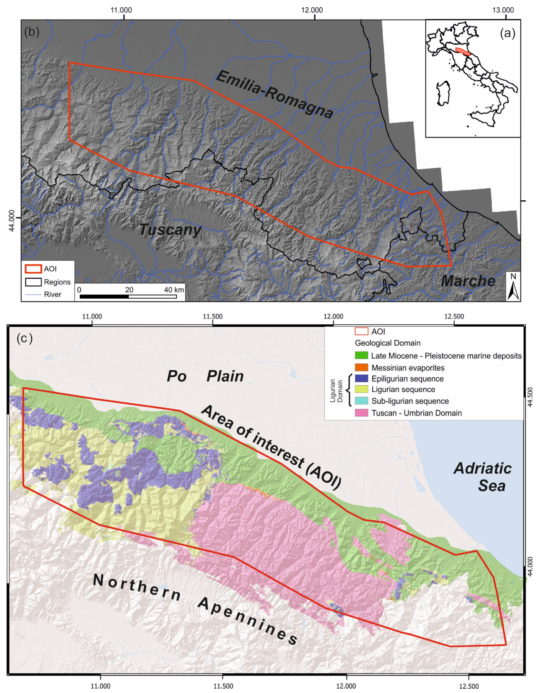
Figure 1 shows the Digital Elevation Model (DEM) of the study area, in Northern Italy, mainly located in the Emilia-Romagna (ER) region. The area of interest (AOI), where we mapped the rainfall-triggered landslides, covers 5764 km2, with elevations ranging between 10 and 1400 m asl. The DEM clearly shows a geomorphological boundary between the plain sector to the NE and the hilly sector of the Northern Apennines to the SW. The main rivers flow from the SW to the NE and reach either the Po River or the Adriatic Sea; in the plain, the rivers flow at elevations higher than the surrounding plain. Such a configuration implies that, following heavy rainfalls, the hilly sector is prone to slope movements, while the plain suffers from flooding.
In the hills, the slopes are generally gentle, with values in the range of 0–70°, with a broad modal peak centered at 10–20°. From the geological point of view, the chain sector of the AOI is the result of the tectonic superposition of two large sets that are different in lithology, structure and paleogeographic origin: an External Umbrian–Tuscan Domain, mainly outcropping to the SE and composed of turbiditic units, well-bedded marls and sandstones, and an Internal Ligurian–Emilian Domain, outcropping to the NW, composed of shales, chaotic melange and flysch-like units [32]. From the lithological point of view, the AOI is characterized by the outcropping of terrigenous formations with a high clay content, alternating sandstones marls and siltstones and turbiditic successions, resulting in a typical landscape characterized by badlands and diffuse slope movements. Lithological control on erosion results in aligned cuestas and hogbacks. Where the superimposition of flysch or sandstones occurs, sub-vertical slopes and mesa-like features are displayed (i.e., the so-called “Pietra di Bismantova”; [33]). The Italian inventory of slope movements [34] includes over 40,000 mapped landslides in the AOI (45% rotational/translational slides and 30% slow earth flows).
The primary land covers, after the Emilia-Romagna region land use database (last updated in 2020, following the CORINE land cover classification scheme [35]), include agricultural fields and forested areas for the hillside sector of the AOI, followed by urbanized land use, mainly located at the foothills or in the plain area.
The mean annual rainfall is in the range 700–1400 mm (the climatic atlas of the Emilia-Romagna region, [36]), with the values increasing from the NE to SW; autumn represents the wettest season, followed by a secondary peak in precipitation in the spring.
2.2. The Rainfall Episodes of May 2023
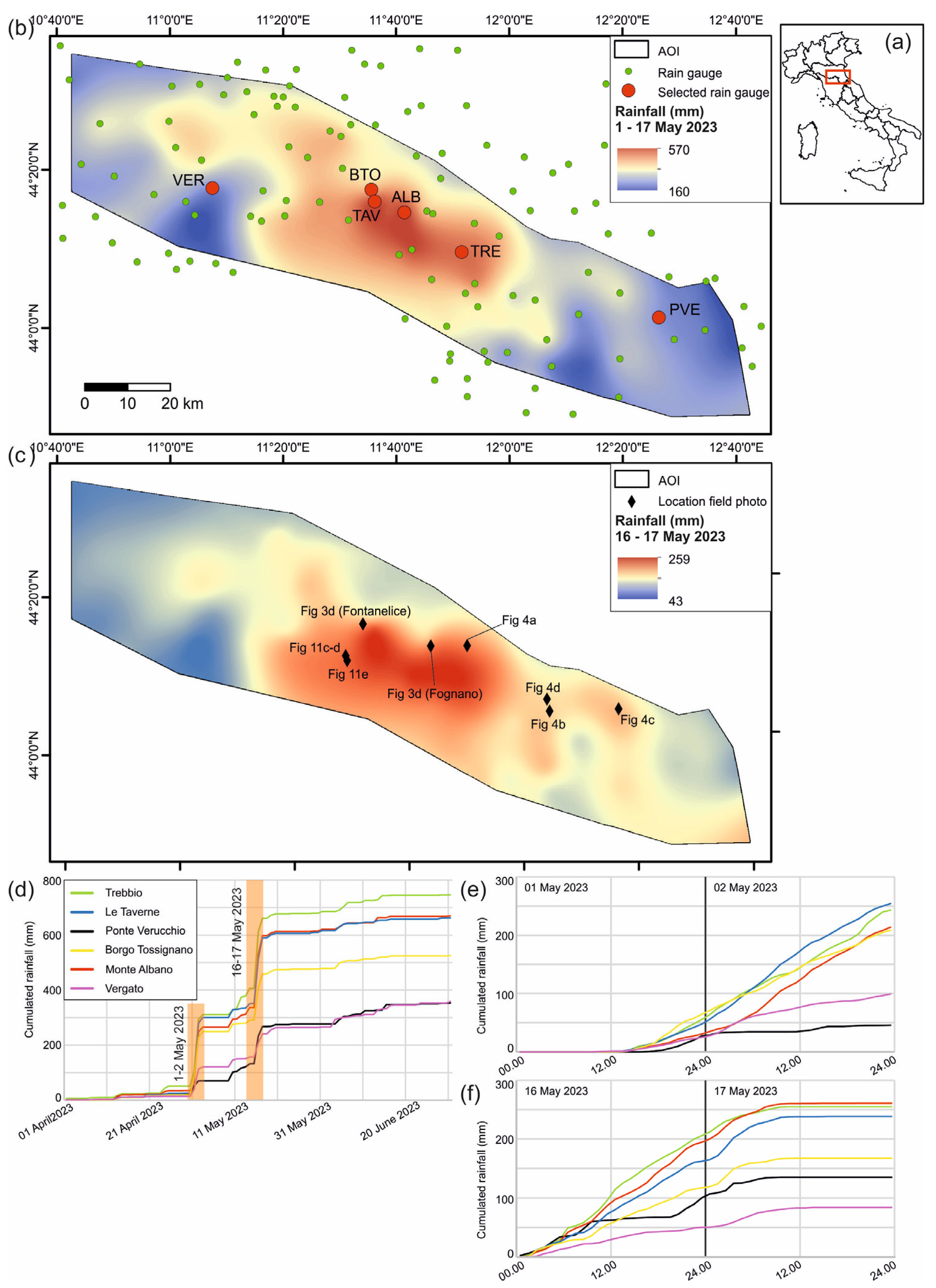
During May 2023, the ER region experienced prolonged and intense rainfall, mainly distributed in two episodes, i.e., 1–2 May and 16–17 May. The gauge records (Figure 2, Table 1) show no significant rainfall in the 30 days preceding the first rainfall episode. At the beginning of May 2023, rainfall hit the entire AOI, with the cumulative values exceeding 200 mm (e.g., 254 mm at Le Taverne and 243 mm at Trebbio). The hourly intensities were generally lower than 3–5 mm/h, with few peaks exceeding 15–20 mm/h. This event was the most intense in a 2-day interval since 1997 and the most intense in the spring season since 1961 [37]. The geographic distribution of the rainfall is shown in Figure 2a. The highest values were recorded in the Reno, Lamone and Montone drainage basins; the precipitation generated an increase in river discharge, reaching hydrometric levels close to, and locally higher than, the levee levels. Sporadic slope movements were triggered as well [37].
An even stronger precipitation event (Minerva storm) occurred on 16–17 May 2023 (Figure 2b); again, the most hit area was the hilly sector of the ER region. The cumulative values over the 2 days reached 260.8 mm at the Monte Albano gauge and 254.8 at Trebbio. The cumulative rainfall over the 17-day period (1–17 May 2023) is the highest historical record for about 65% of the gauge stations in central and eastern ER [38]; the maximum values reached 609.8 mm at Trebbio and 563.4 mm at Le Taverne (Figure 2c). The high discharge resulted in extensive floods of the plains and in thousands of landslides in the hills.
3. Materials and Methods
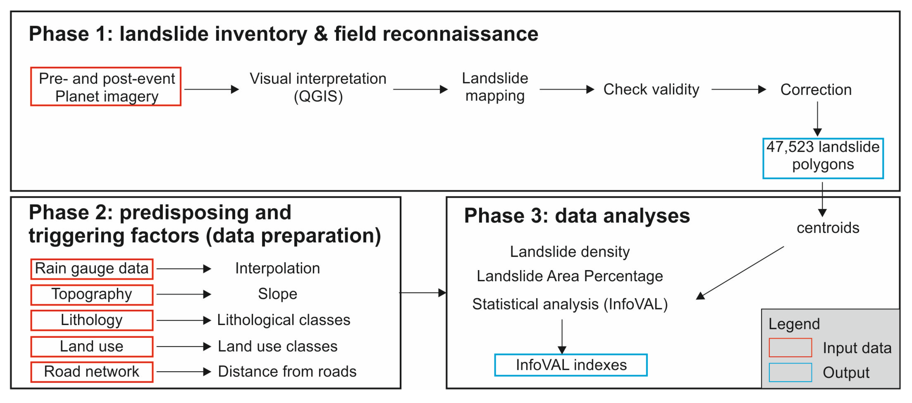
Figure 3 represents the methodological workflow adopted in this study. The approach consists of three subsequent phases, namely, (i) building the landslide inventory and performing the field reconnaissance, (ii) acquiring data on predisposing and triggering factors and (iii) conducting data analyses. At each step, input data are required, which may be obtained from external sources (e.g., satellite images and thematic maps) or generated in the previous steps (e.g., landslide polygons).
3.1. Realization of the Landslide Inventory
The first step of this research is the realization of the landslide inventory, which is based on a visual inspection of pre- and post-event satellite images in an area of 5764 km2. The satellite images were acquired by PlanetScope (https://www.planet.com/, last accessed on 3 November 2023) and were provided under an academic license as ortho-rectified products; 3 m resolution multiband tiles were used. A screening of the available imagery was initiated within hours of the 16–17 May precipitation episode, using the Planet website; for a few days the area was heavily clouded, and the first cloud-free images were available on 22 May. For the realization of the inventory, the images were accessed through the Planet QGIS Plugin; the pre-event imagery refers to the Monthly Global Basemap products provided by Planet, and the April 2023 Basemap was used. The post-event images were acquired between 22 May and mid-June 2023. The cloud-free image closer to the event was used and multitemporal frames were checked in the selected areas (e.g., due to the presence of shadows or unclear images).
The landslides were manually mapped at a scale of 1:5000 by a single operator in a time interval of 5 weeks following the rainfall event; the inventory (version 1.0) was released online on 28 June 2023. The landslides were mapped as polygons encompassing both the source and deposit areas, because they are not easily discernible in satellite images; the landslides were mapped as individual polygons as much as possible, trying to avoid issues related to amalgamation [39].
We realized the field surveys in a limited subset of the AOI on 30 July–1 August 2023; we drove along the main and secondary roads, and we acquired photographic documentation of the landslides at selected spots along the roads or at scenery points for a broader view.
We computed the area–frequency distribution of the event inventory following [40]. The probability density for classes of a width equal in logarithmic coordinates is calculated as:
where N is the total number of landslides, and NL is the number of landslides with an area between AL and AL + δAL.
3.2. Predisposing and Triggering Factors
The second step of the research includes the acquisition and preparation of the thematic data related to the predisposing and triggering factors. We compared the spatial distribution of the landslides with some descriptors of the local geological and geomorphological setting and with the spatial distribution of the precipitations during the May 2023 events. We selected five influencing factors for further analyses, namely, rainfall, slope, land use, lithology and distance from roads.
We interpolated the pluviometric data published in the ER report [38]. The cumulative pluviometric data refer to the period 1–17 May 2023 and for the two-day period of 16 and 17 May 2023. We interpolated the point data with a local polynomial interpolator algorithm (spline interpolation) to grant the representativeness of the data in terms of local trends and to avoid possible spikes in the data distribution.
For the topographical analyses, we used the 20 m DTM of Italy, released by ISPRA, and we derived the slope values (in degrees).
We obtained a lithological map of the area from the ER region WebGIS at a 1:50,000 scale. The geological map has been directly derived from the Italian national geological cartography program (CARG Project) and includes a lithological classification of each geological unit. For the sake of simplicity, we adopted the classification scheme summarized in Table 2.
Land use was downloaded from the ER region WebGIS. This database follows the CORINE land cover hierarchical classification scheme and was updated in 2020. We compared the occurrence of landslides with the main categories of land use as summarized in Table 3.
To estimate the possible influence of the vicinity of roads for landslide triggering, we used the Open Street map database of roads and streets, including all the road types except for paths in mountain areas.
3.3. Data Analysis
The last part of our work is dedicated to the statistical analysis of the inventory. As a first step, we carried out a topological check on the landslide inventory using the “check validity” QGIS tool to correct auto-intersecting polygons; this check resulted in 14 invalid polygons (0.03% of the mapped landslides), which were manually corrected. To investigate the spatial distribution of landslides, we computed the landslide number density (LND) and landslide area percentage (LAP), which later were statistically analyzed with respect to predisposing and triggering factors.
The landslide density was calculated by means of the kernel density estimation approach using a kernel density estimator (KDE) in a GIS environment (e.g., [41,42]). The KDE calculates the density of point features if a probability density function of event occurrence (i.e., the kernel shape) is centered at the observation point. The probability diminishes with increasing distance from the point, reaching zero at the search radius distance (h) from the point. Only a circular neighborhood is possible.
Following [43], we calculated h according to the following formula:
where IQR and SD are the interquartile range and the standard deviation, respectively, of the distances between each observation point and the centroid of the point population; n is the number of points.
The density at each output raster cell is calculated by adding the values of all the kernel surfaces where they overlay the raster cell center. We adopted an Epanechnikov kernel shape [44], namely, a kernel function built as the positive part of a parabola that minimizes the errors associated to the tails of the estimates [43]. We also produced a density raster of the calculated KDE density with 100 m cell spacing.
LAP represents the percentage of the territory covered by the rainfall-triggered landslides; it was computed on a regular grid of cells having an area of 1 km2.
The quantitative relationship between landslides and predisposing factors affecting landslides are established by the data-driven Information Value (InfoVAL) method [45,46,47]. The method allows for the quantified prediction of susceptibility by means of a score (Wi), calculated according to landslide occurrence on each class and weighed according to the class distribution over the entire study area:
where Wi is the score for the i-th class, Densclass is the landslide occurrence for the i-th class and Densmap is the i-th class occurrence on the whole area. This formula normalizes the event occurrences over the spatial distribution of each considered class. Positive values indicate a positive statistical correlation and negative values a negative one, while values close to zero indicate a random distribution of the data. We applied the InfoVAL method to the territory of the ER region, where consistent and homogenous information is available. Emilia-Romagna accounts for 97% of the mapped landslides, so we claim that the obtained results can be considered representative of the entire dataset.
4. Results
4.1. The Inventory
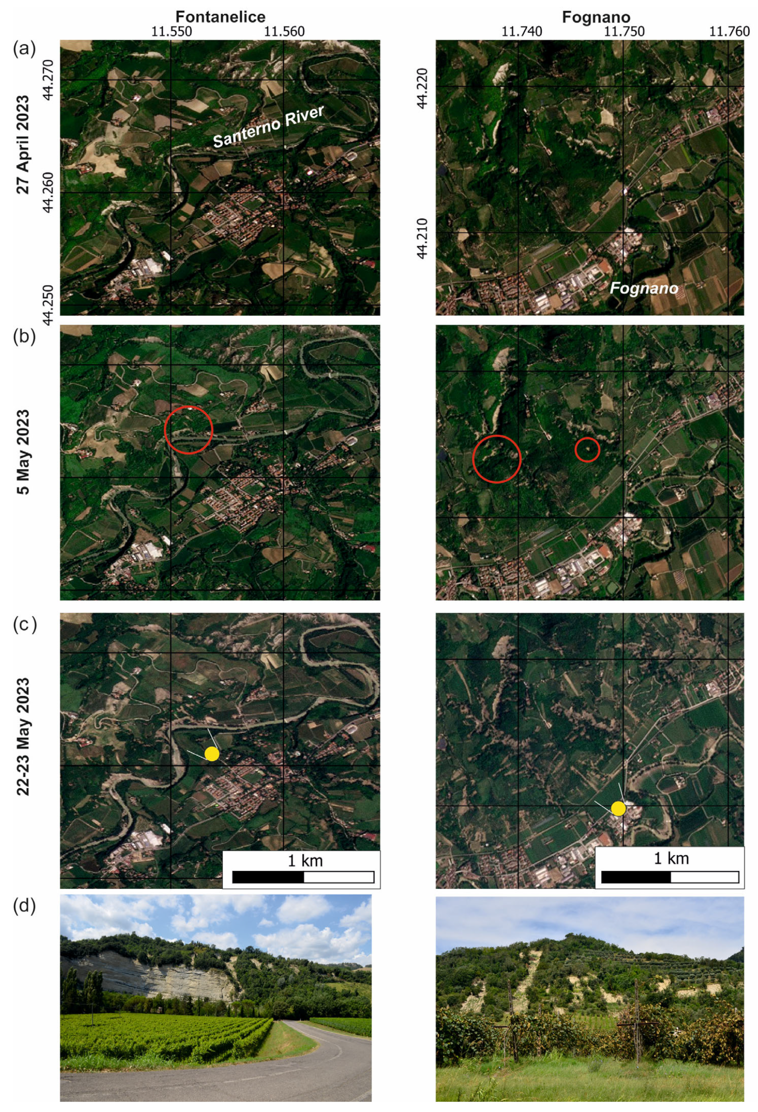
The dataset contains 47,523 landslides in an area of 5764 km2, corresponding to an average density of about 8 landslides/km2. Figure 4 shows two examples of multitemporal satellite images at the localities of Fontanelice and Fognano (for the location, see Figure 2c). The upper panels (Figure 4a) represent the images acquired before the rainfall episodes, i.e., on 27 April; the mid-panels (Figure 4b) were acquired after the first rain spell, i.e., on 5 May; and the lower panels (Figure 4c) were acquired a few days after the main rainfall episode, i.e., on 22–23 May. Finally, Figure 4d presents two field photographs of the sites.
The pre-event images provide an overview of the typical local setting, which includes a variable proportion of urban areas, agricultural fields, woodlands and outcropping rocks. From the comparison of the multitemporal images, it is evident that most of the landslides occurred after the 16–17 May rainfall episode; nevertheless, a few landslides are recognizable on the 5 May images as well (see red circles), mostly related to the reactivation of pre-existing slope movements. The landslides are not homogeneously distributed but tend to cluster at specific places, such as along the Santerno River (Fontanelice) or in the woodland and cultivated fields N of Fognano. The field photos show the occurrence of closely spaced slope movements with variable runouts, which scraped off the vegetative cover.
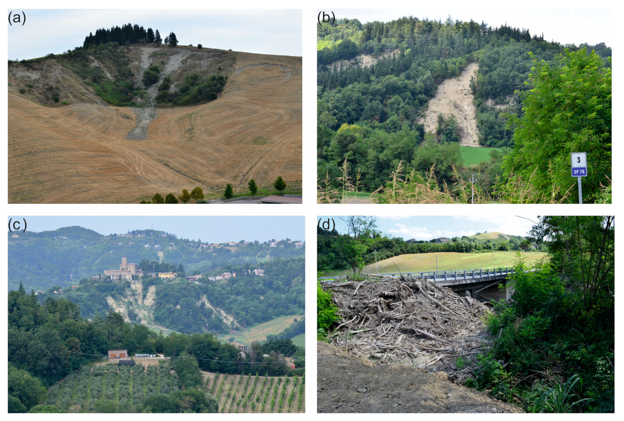
Figure 5 presents the selected examples of the landslides observed in the field and having variable characteristics in terms of the size, shape, geomorphological setting and involved materials. The location of the sites is presented in Figure 2c. Figure 5a includes two slides with long runouts coalescing into a single toe; the crown areas are at the top of a small hill, while the toe intersects an agricultural field. Figure 5b shows a single slope movement on the lower part of a steep slope in a vegetated region; in this case, the deposit area lies at the base of the slope. Figure 5c shows a panoramic view of the multiple landslides that occurred on the slope beneath the Sorrivoli Castle, a fortress built in the XI century. Figure 5d shows the trunks and sediments transported by a river course and deposited at the intersection with a road bridge. Figure 5c,d represent typical interactions between the landslide events or destabilized material and anthropic activities, infrastructures or cultural heritage.
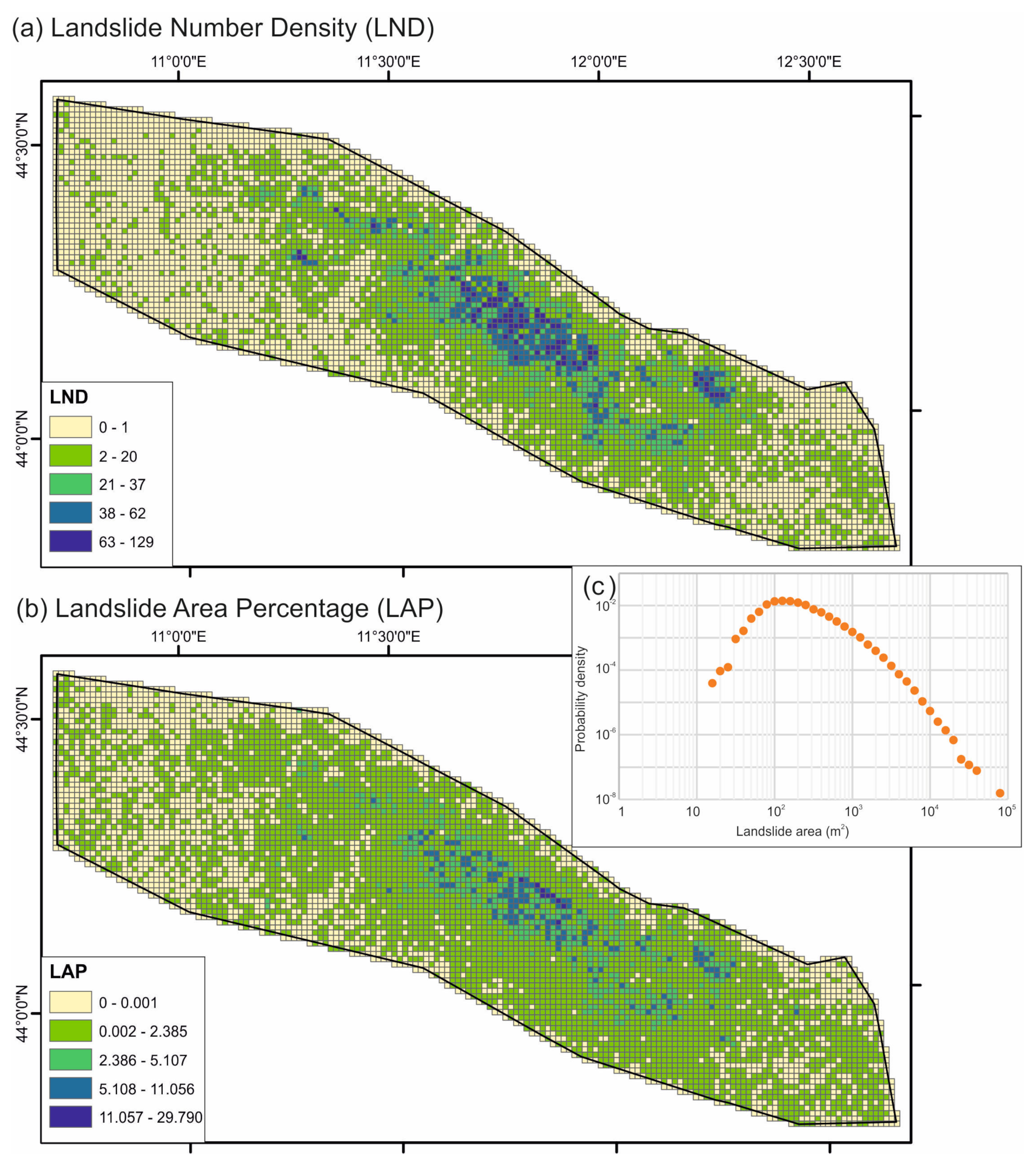
The dataset is entirely original, and the shapefiles (coordinate system WGS84 UTM 32N) can be publicly accessed at https://zenodo.org/record/8102429 (last accessed 1 October 2023). We computed the LND and LAP values on a regular grid of cells having a dimension of 1 km2. Figure 6 allows for appreciating the uneven spatial distribution of the landslides: the highest LND and LAP values are indeed located in a small portion in the central part of the AOI and decrease moving outwards. The maximum LND values reach 129 landslides/km2, while the maximum LAP values reach around 30%.
The landslide polygons cover an area of 40.9 km2, which represent 0.71% of the AOI; the largest mapped failure has an area of 98,000 m2, while the average area is 860 m2. The probability density of the dataset is presented in Figure 6c: the curve is characterized by the typical pattern of other landslide–area distributions, namely, a negative power law fit for medium to large landslides and a positive power law fit for small to medium landslides. The two limbs of the curve are separated by a rollover, which in our case is located at a size of 120–150 m2. The exponent of the negative power law is −2.22, which is in broad agreement with other inventories worldwide [18,23,26,48].
4.2. Predisposing and Triggering Factors
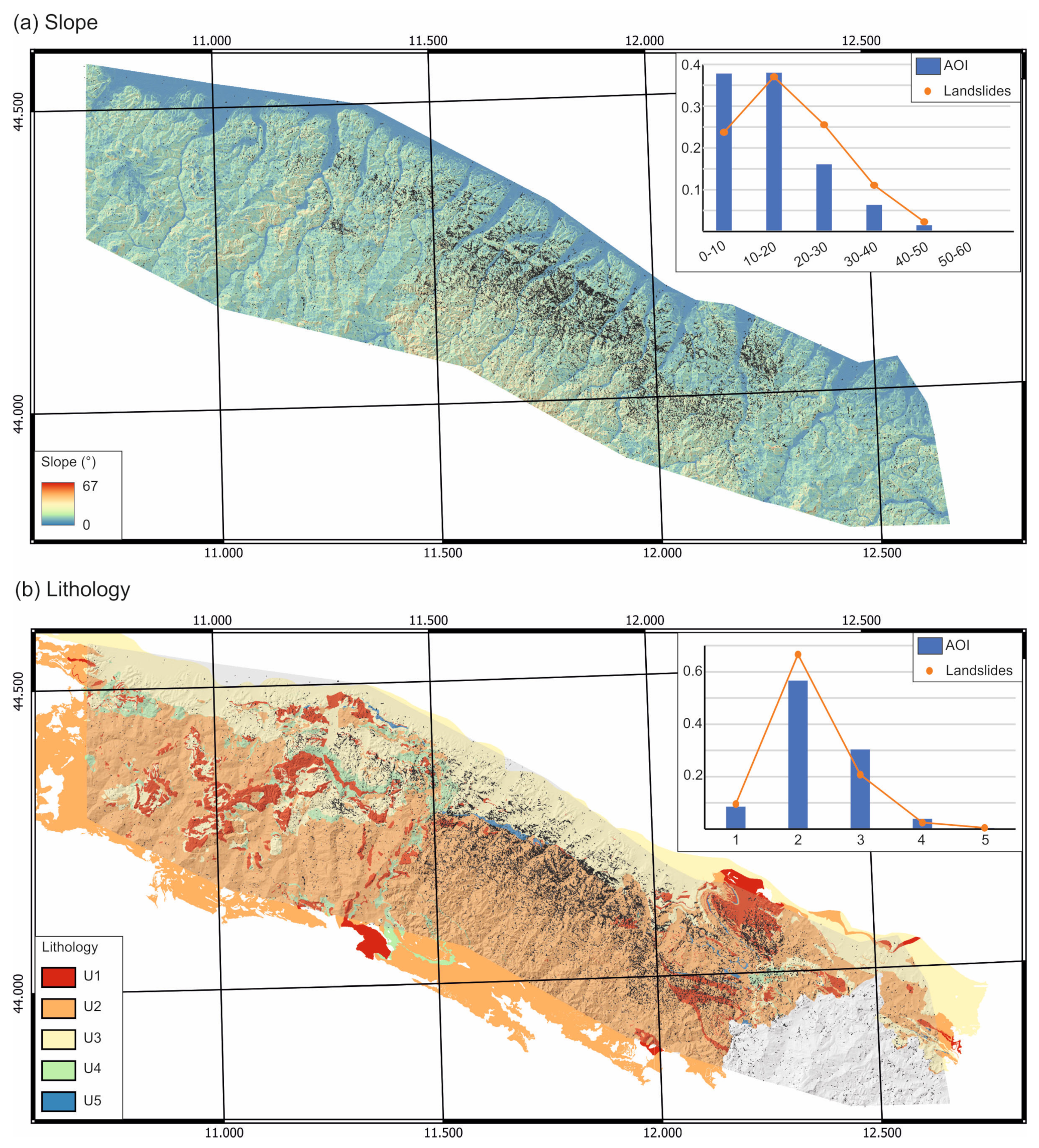
We selected four predisposing factors for the subsequent analysis; one is related to the topography (i.e., slope) and one to the geologic setting (lithology), while the remaining two factors are the land use and distance from roads, which account for the anthropic territorial modifications. Figure 7 and Figure 8 show the maps of the four factors, while the categories used to classify the lithology and land use are presented in Table 2 and Table 3, respectively. The plots in the upper-right corner of Figure 6 and Figure 7 show the repartition among the different units: the overall AOI is represented by the blue columns, while the orange dots represent the proportion of landslide centroids falling within each unit.
Figure 7a presents the role of the slope, which has been categorized into units of 10° width. Categories 0–10° and 10–20° share an almost equal amount of the AOI (38% each), but the landslide centroids peak in the 10–20° class, with a value of 37%. The steeper slopes are less diffuse in the AOI, but the landslide centroids are over-represented, especially in the 20–30° and 30–40° classes.
Figure 7b presents the role of lithology, which has been categorized into five units (see Table 2). The most represented unit in the AOI comprises “siltstones, marls and limestones interbedded with marls”; it covers 57% of the AOI, and 67% of the landslide centroids lie within Unit 2. Overall, the abundance of landslides for each unit follows the lithological repartition in the AOI.
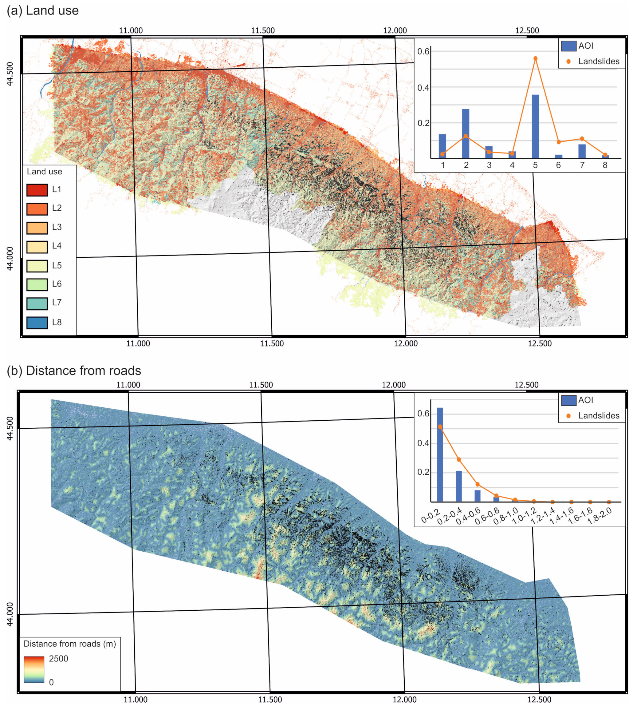
Figure 8a presents the role of land use, which has been categorized into eight units (see Table 3). The most represented unit in the AOI is L5 (i.e., woods, 36%), followed by L2 (arable land, 28%). When considering landslide centroids, more than half (56%) lie in Unit L5, pointing toward a strong influence of this land use category. Unit L6, bare rocks and badlands, accounts for only 2.2% of the AOI but includes 9% of the landslides, again suggesting that it may be a strong predisposing condition. On the contrary, Unit L1 (urban areas) covers 14% of the AOI, but only 2% of the landslides are located in Unit L1, probably because urban areas lie on flat regions and/or landslides are more difficult to identify in satellite imagery.
Figure 8b presents the role of the distance from roads, which has been categorized into units of 200 m width. The AOI shows an exponential decrease with distance: 86% of the AOI lies at less than 400 m from a road, testifying to the high density of infrastructures and thus the exposed assets. The distribution of landslide centroids mimics the AOI repartition, because the most represented class is within 200 m from a road (51%).
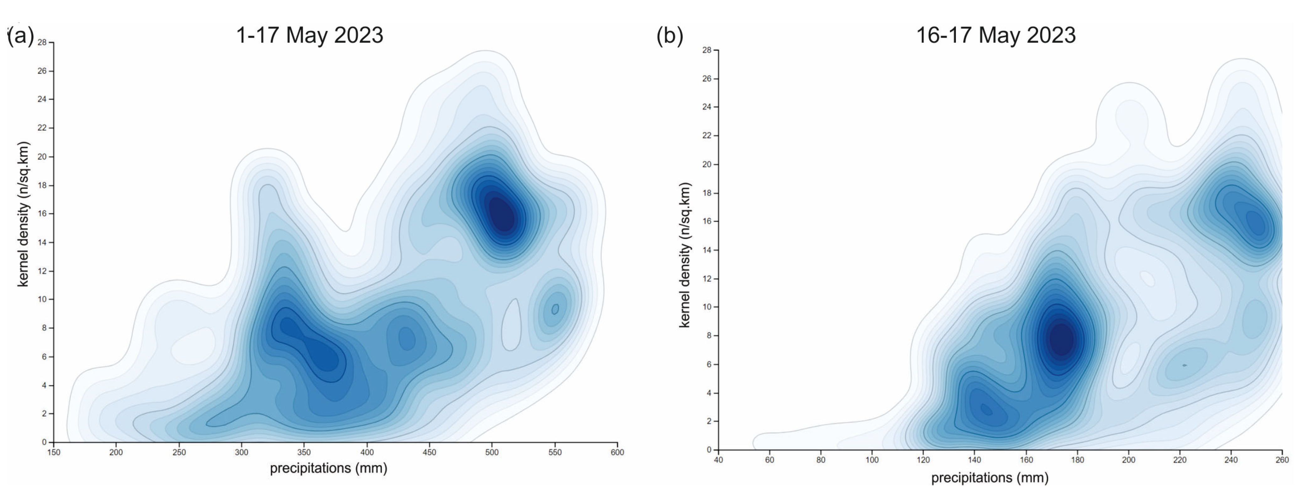
Precipitation is the triggering factor of this large amount of mass movements. A comparative analysis between the landslide KDE value and the corresponding precipitation, occurring at the same location, provides some additional insights. We considered both the distribution of the cumulative precipitations that occurred during the whole rainfall period (1–17 May 2023; Figure 9a) and the precipitations that occurred during the second rainfall event alone (16–17 May 2023; Figure 9b). Even considering a quite scattered distribution of the datapoints, it is apparent that there is a good positive correlation between the amount of rainfall and the spatial density of landslides. In particular, if we consider the 16–17 May 2023 event alone, the graph points to a threshold value for the inception of landslides of ca. 120 mm over the considered period.
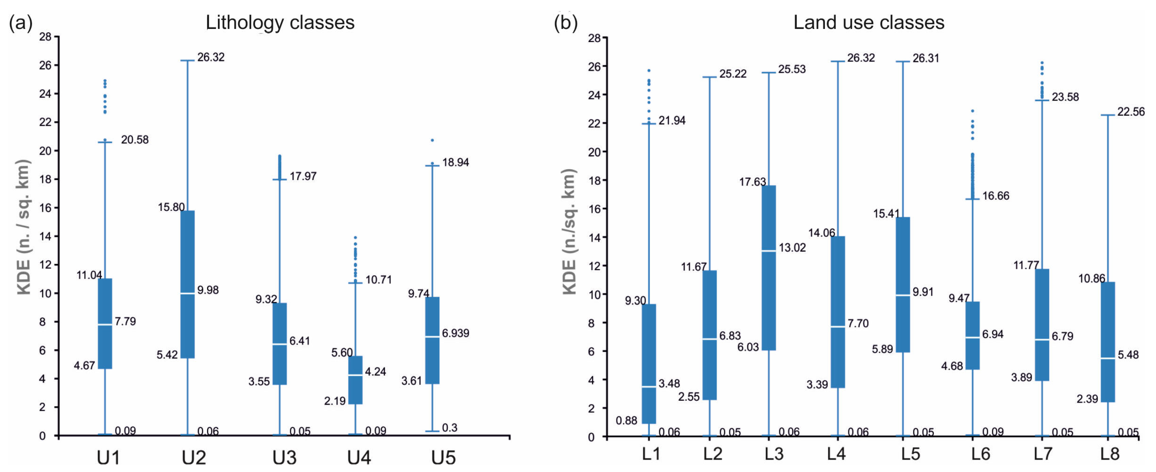
The analysis of the frequency distribution of the landslide KDE value for each land use and lithology class highlights how the landslides concentrate or not in certain zones (Figure 10). A lithological control on landslide occurrence is apparent only for conglomerate-like units (class U4), inhibiting the massive landsliding, and flysch-like units (class U2) that, on the contrary, look to host a higher landslide density.
As for the land use, agricultural land (class L3) and woodland (class L5) are correlated to an average higher KDE value, also considering a quite broad distribution of values. On the other hand, urban areas (class L1), on average, are the only ones less affected by landsliding.
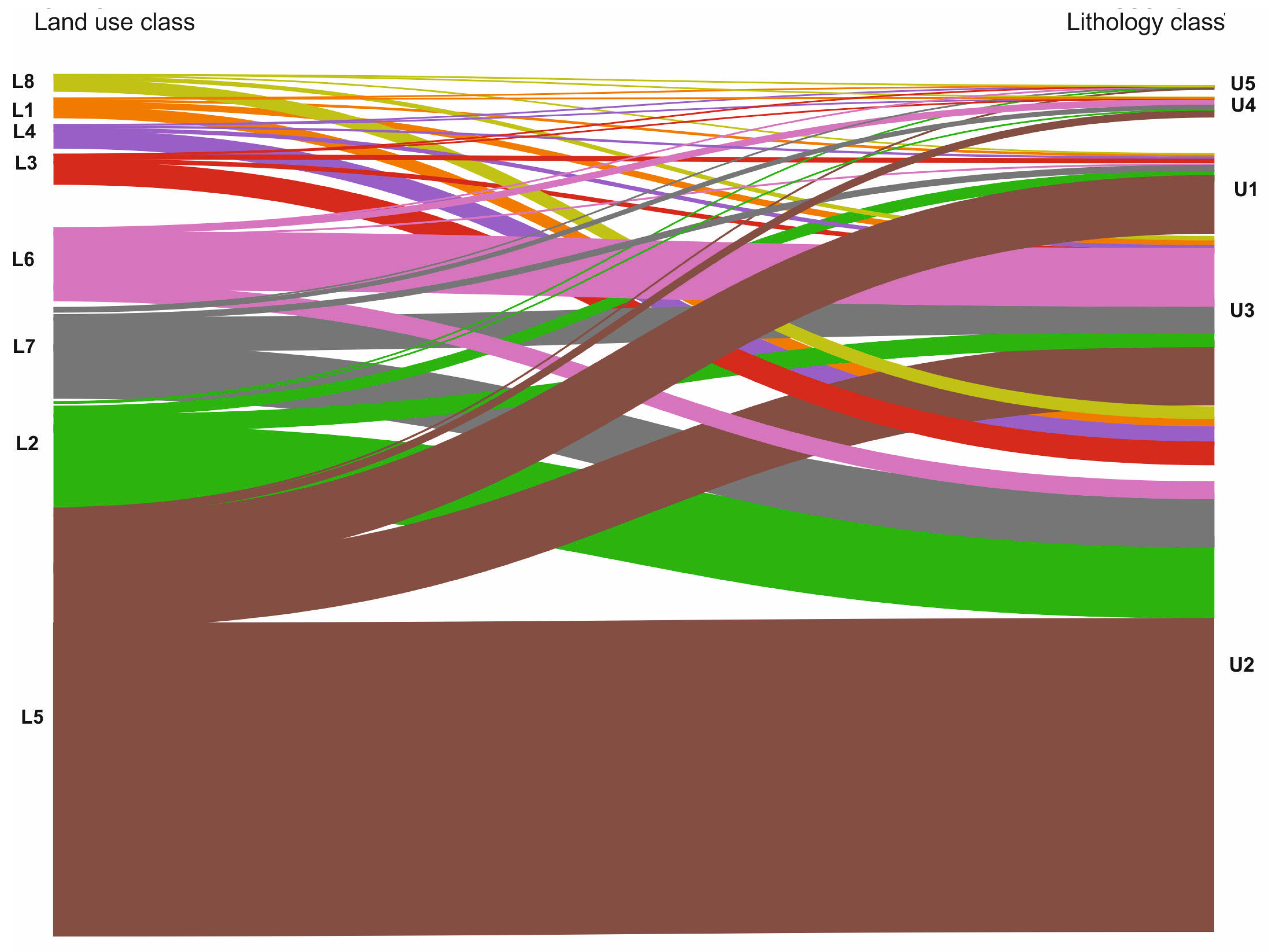
Finally, if we check the relative representation of the land use and lithology classes, and the reciprocal exchange of events among those classes (Figure 11), we can appreciate that, overall, most landslides belong to woodland (class L5) over flysch-like units (class U5), with most of the remaining landslides from the woodland distributed between the sandstones (class U3) and limestone (class U1) units. Flysch-like units are also associated with a considerable number of events that happened on arable land (class L2) and shrubs (class L7).
Another considerable number of events belong to bare lands (L6) on sandstones (U3) and to woodland (class L5) on limestones (class U1).
4.3. InfoVAL Analysis
From the calculated InfoVAL index (Table 4), it is apparent that lithology has a moderate effect on predisposing the slopes to landsliding: positive Wi values are associated with silty and flysch-like units, but only small positive correlations can be supposed. On the other hand, sandstones represent a more stable terrain over which landsliding is inhibited. The land use classes predisposing landsliding are woods and shrubs, with a striking high value associated with bare rocks and badlands. The slope classes are particularly indicative of a susceptibility between 20° and 40° and for extremely high values (60–80°).
Finally, the distance from roads is somehow indicating an augmented hazard in the range of 200–800 m. The majority of landslides mapped in our study lie within 200 m from a road. This result is consistent with those obtained by [28], who realized an inventory of 1687 landslides triggered by a rainfall episode that occurred in the Umbria and Marche regions on 15 September 2022. They found that 60% of the mapped landslides lie within 50 m from the roads, and the percentage grows to 89% within 200 m from the roads. It is important to note that the methods of [28] are different from the ones used here: indeed, they realized the extensive reconnaissance field surveys by driving along main and secondary roads and stopping at every landslide or scenery point.
5. Discussion
5.1. Comparison with Other Case Studies
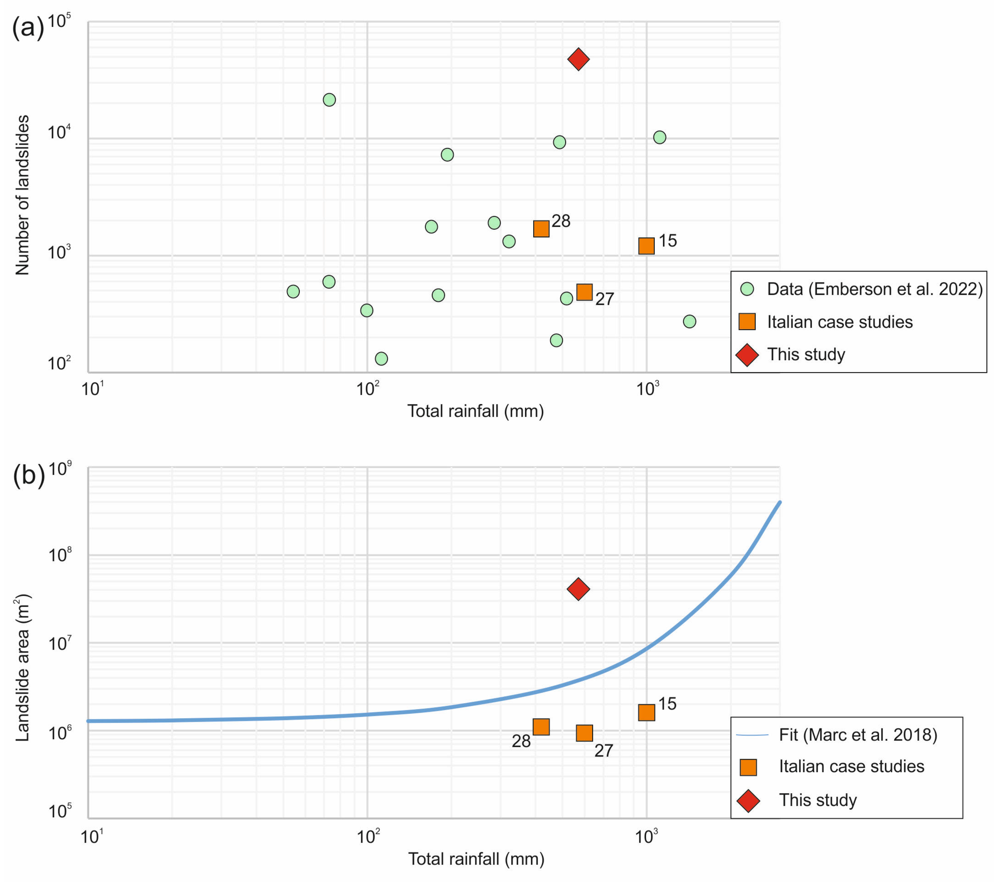
The inventory presented in this study includes 47,523 landslides, thus representing one of the most numerous event inventories on a global scale. Here, we compare the figures of the Emilia-Romagna inventory with other case histories available in the literature to look for common patterns or, on the contrary, peculiarity in the case study presented here. Comparative studies have been realized on a dataset of 16 inventories pertaining to events that occurred between 2002 and 2019 [18,23]. The events cover a variety of precipitation patterns (cyclones, typhoons, local storms and prolonged intense rainfall) and geographic settings (Central and South America, East Africa, India and East Asia). The total event rainfall ranges between 45 and 2500 mm. A strong influence on the triggered landslides is played by the total storm rainfall, while topographic parameters (e.g., slope) have a lower impact [18]. Overall, a non-linear increase in total landsliding is observed with respect to total rainfall. The number of triggered landslides also scales with the total rainfall amount, although the scatter is higher; this latter point can be due to the fact that the inventories were delineated on images with a different resolution [18].
As a comparison, we recall that the rainfall in the Emilia-Romagna region reached 254 mm on 1–2 May 2023 and 260 mm on 16–17 May 2023, while the cumulated rainfall over the entire period (1–17 May 2023) was about 570 mm. These figures suggest that the case study presented here is consistent with the literature data.
Figure 12a presents the number of landslides versus the total rainfall amount for the dataset by [23], while Figure 12b presents the empirical relationship between the total rainfall and the landslide area presented by [18]. We supplemented the graph with three Italian case histories [15,27,28] and with the inventory presented in this study. It is quite evident that the Emilia-Romagna case history plots well above previous investigated events. Several factors may account for such a difference, including (i) the fact that the case study presented here was particularly effective in triggering landslides, or (ii) there is an issue of completeness in the landslide mapping, or (iii) there is some fundamental difference in the considered events or methodological assumptions. We prefer the former two hypotheses, because some of the inventories in the literature were derived from the same kind of satellite imagery and with comparable methods; the frequency–area distribution of the Emilia-Romagna inventory has a rollover at ca. 120–150 m2, while the inventories have rollovers ranging between 102 and 103 m2, suggesting that our inventory contains a larger number of small landslides.
5.2. Limitations of the Inventory
Here, we highlight some critical aspects and limitations of our study, related either to the methodological mapping and analytical choices, or actual limitations in the input data.
In the first days after the 16–17 May rainfall episode, persistent cloud cover hampered the identification of landslides; the inventory is thus based on multitemporal images acquired on different dates. The high revisit time of the Planet images allows for closely bracketing the time of occurrence of the landslides. Figure 2d shows that no significant rainfall occurred after the 16–17 May episode; nevertheless, we cannot rule out that some slope movements may have been triggered a few days after the rainfall episode. The same reasoning applies to landslides that may have occurred in the first half of May (i.e., after the 1–2 May rainfall): Figure 4 shows that most of the movements have been triggered after the 16–17 May rainfall, but some landslides may have been mobilized before that episode. Overall, our inventory has to be intended as the cumulative effect of both the 1–2 and 16–17 May rainfall spells.
The inventory was released on 28 June 2023, i.e., 1.5 months after the main triggering event; in this sense, our inventory can be assimilated to rapid response products (e.g., [49]). Some operative choices represent a trade-off between the rapidity of execution and data quality/resolution, for instance, the mapping was realized at a 1:5000 scale and should be consulted at most at the same scale; a side effect is that our mapping is not recommended for higher resolution susceptibility studies, unless a field verification is undertaken. We underline that our inventory is one of the few that have been publicly released; to our knowledge only one other inventory has been published to date, realized through automatic mapping from Sentinel-1 images ([50]; publication date 1 June 2023).
The investigated AOI is 5764 km2 wide, meaning that the inventory does not entirely cover the area hit by rainfall. However, we argue that the inventory effectively captures the worst hit area and represents a significant snapshot of the event.
We expect that our inventory may contain a certain number of false positives, especially in agricultural fields, built-up areas or close to riverbanks; indeed, in the post-event imagery, such areas show spectral characteristics similar to landslide areas (e.g., [10,11]). We also expect some completeness issues (false negatives) in the vicinity of roads and river networks: our limited field surveys allow us to ascertain the occurrence of a high number of slope movements affecting the road network. Figure 13 presents some representative cases of field photos and satellite images: the two areas shown in Figure 13a,b lie about 1 km apart on Province Road SP610 in the Castel del Rio Municipality. In the first case (Figure 13a,c,d), the slope movement is clearly visible in the satellite image and is included in the inventory; the landslide intercepts the road and flows down, reaching the Santerno River course. In the second case (Figure 13b,e), a small slope movement occurred along the road bank; this landslide is not visible in the 3 m resolution Planet image and thus is not included in our inventory. The latter example suggests that the abundance of slope movements within 200 m from roads (see Figure 8b) may be underestimated. The high influence of a dense road network as a predisposing factor for landslides has been already pointed out in previous studies (e.g., [51]).
Finally, we highlight that very limited field verification has been realized so far and no systematic evaluation of the reliability and accuracy of the inventory has been carried out. Indeed, the quality and reliability of the inventory control the overall quality of derivative products, such as the susceptibility and risk assessment [52,53]. Such aspects are beyond the scope of this paper but should be addressed whether the inventory presented here is used as input data for further studies.
6. Conclusions
In this paper, we present an inventory of 47,523 landslides triggered by heavy rainfall that occurred in May 2023 in the Emilia-Romagna and conterminous regions (Italy). A first precipitation episode occurred on 1–2 May 2023 and a second one on 16–17 May; the latter was responsible for most of the observed landslides.
The inventory was realized by a visual inspection of the pre- and post-event satellite imagery with a resolution of 3 m. The adopted methods are standard practice, and our effort is devoted to filling the data gap existing for the investigated triggering event. A limited field survey at selected locations was conducted to validate the inventory. We statistically investigate the relationship between landslide density and triggering (precipitation) and predisposing factors using the InfoVAL method. A strong influence is due to steep slopes and some land use categories (bare rocks and badlands, and woodlands), while a weaker positive correlation is found with respect to lithology because a higher landslide density is obtained for silty and flysch-like units.
The inventory presented here is one of the most numerous on a global scale and we argue that it can support the validation of other products, for instance, that are obtained through automatic mapping methods. The statistical results on triggering and predisposing factors may be useful for susceptibility assessment and land planning (e.g., landslide zoning) or the derivation of empirical rainfall thresholds for landslide triggering.
Author Contributions
Conceptualization, M.F.F. and F.L.; methodology, M.F.F. and F.L.; formal analysis, M.F.F. (realization of the inventory) and F.L. (analysis of influencing factors); investigation, M.F.F. and F.L.; writing—original draft preparation, M.F.F.; writing—review and editing, M.F.F. and F.L. All authors have read and agreed to the published version of the manuscript.
Funding
This research received no external funding.
Data Availability Statement
The landslide inventory realized in this study is publicly available at https://zenodo.org/record/8102429, last accessed 1 October 2023. Rainfall data retrieved from https://simc.arpae.it/dext3r/, last accessed 1 October 2023. Ancillary data for the Emilia-Romagna region can be downloaded at https://geoportale.regione.emilia-romagna.it/, last accessed 1 October 2023.
Acknowledgments
We wish to thank the Assistant Editor and three anonymous reviewers for their comments, which improved the quality of the manuscript.
Conflicts of Interest
The authors declare no conflicts of interest.
References
- Cruden, D.M.; Varnes, D.J. Landslide types and processes. In Landslides, Investigation and Mitigation, Special Report 247; Turner, A.K., Schuster, R.L., Eds.; Transportation Research Board: Washington, DC, USA, 1996; pp. 36–75. ISBN 030906208X. [Google Scholar]
- Hungr, O.; Leroueil, S.; Picarelli, L. The Varnes Classification of Landslide Types, an Update. Landslides 2014, 11, 167–194. [Google Scholar] [CrossRef]
- Froude, M.J.; Petley, D.N. Global Fatal Landslide Occurrence from 2004 to 2016. Nat. Hazards Earth Syst. Sci. 2018, 18, 2161–2181. [Google Scholar] [CrossRef]
- Haque, U.; Blum, P.; Da Silva, P.F.; Andersen, P.; Pilz, J.; Chalov, S.R.; Malet, J.-P.; Auflič, M.J.; Andres, N.; Poyiadji, E.; et al. Fatal Landslides in Europe. Landslides 2016, 13, 1545–1554. [Google Scholar] [CrossRef]
- Salvati, P.; Bianchi, C.; Rossi, M.; Guzzetti, F. Societal Landslide and Flood Risk in Italy. Nat. Hazards Earth Syst. Sci. 2010, 10, 465–483. [Google Scholar] [CrossRef]
- Haque, U.; Da Silva, P.F.; Devoli, G.; Pilz, J.; Zhao, B.; Khaloua, A.; Wilopo, W.; Andersen, P.; Lu, P.; Lee, J.; et al. The Human Cost of Global Warming: Deadly Landslides and Their Triggers (1995–2014). Sci. Total Environ. 2019, 682, 673–684. [Google Scholar] [CrossRef] [PubMed]
- Guzzetti, F.; Mondini, A.C.; Cardinali, M.; Fiorucci, F.; Santangelo, M.; Chang, K.-T. Landslide Inventory Maps: New Tools for an Old Problem. Earth-Sci. Rev. 2012, 112, 42–66. [Google Scholar] [CrossRef]
- Fell, R.; Corominas, J.; Bonnard, C.; Cascini, L.; Leroi, E.; Savage, W.Z. Guidelines for Landslide Susceptibility, Hazard and Risk Zoning for Land Use Planning. Eng. Geol. 2008, 102, 85–98. [Google Scholar] [CrossRef]
- Corominas, J.; VanWesten, C.; Frattini, P.; Cascini, L.; Malet, J.-P.; Fotopoulou, S.; Smith, J. Recommendations for the quantitative analysis of landslide risk. Bull. Eng. Geol. Environ. 2014, 73, 209–263. [Google Scholar] [CrossRef]
- Martha, T.R.; Kerle, N.; Jetten, V.; Van Westen, C.J.; Kumar, K.V. Characterising Spectral, Spatial and Morphometric Properties of Landslides for Semi-Automatic Detection Using Object-Oriented Methods. Geomorphology 2010, 116, 24–36. [Google Scholar] [CrossRef]
- Mondini, A.C.; Chang, K.-T.; Yin, H.-Y. Combining Multiple Change Detection Indices for Mapping Landslides Triggered by Typhoons. Geomorphology 2011, 134, 440–451. [Google Scholar] [CrossRef]
- Li, Z.; Shi, W.; Myint, S.W.; Lu, P.; Wang, Q. Semi-Automated Landslide Inventory Mapping from Bitemporal Aerial Photographs Using Change Detection and Level Set Method. Remote Sens. Environ. 2016, 175, 215–230. [Google Scholar] [CrossRef]
- Scaioni, M.; Longoni, L.; Melillo, V.; Papini, M. Remote Sensing for Landslide Investigations: An Overview of Recent Achievements and Perspectives. Remote Sens. 2014, 6, 9600–9652. [Google Scholar] [CrossRef]
- De Vita, P.; Reichenbach, P.; Bathurst, J.C.; Borga, M.; Crosta, G.; Crozier, M.; Glade, T.; Guzzetti, F.; Hansen, A.; Wasowski, J. Rainfall-Triggered Landslides: A Reference List. Environ. Geol. 1998, 35, 219–233. [Google Scholar] [CrossRef]
- Guzzetti, F.; Cardinali, M.; Reichenbach, P.; Cipolla, F.; Sebastiani, C.; Galli, M.; Salvati, P. Landslides triggered by the 23 November 2000 rainfall event in the Imperia Province, Western Liguria, Italy. Eng. Geol. 2004, 73, 229–245. [Google Scholar] [CrossRef]
- Kirschbaum, D.B.; Adler, R.; Hong, Y.; Hill, S.; Lerner-Lam, A. A Global Landslide Catalog for Hazard Applications: Method, Results, and Limitations. Nat. Hazards 2010, 52, 561–575. [Google Scholar] [CrossRef]
- Tsai, F.; Hwang, J.-H.; Chen, L.-C.; Lin, T.-H. Post-Disaster Assessment of Landslides in Southern Taiwan after 2009 Typhoon Morakot Using Remote Sensing and Spatial Analysis. Nat. Hazards Earth Syst. Sci. 2010, 10, 2179–2190. [Google Scholar] [CrossRef]
- Marc, O.; Stumpf, A.; Malet, J.-P.; Gosset, M.; Uchida, T.; Chiang, S.-H. Initial Insights from a Global Database of Rainfall-Induced Landslide Inventories: The Weak Influence of Slope and Strong Influence of Total Storm Rainfall. Earth Surf. Dyn. 2018, 6, 903–922. [Google Scholar] [CrossRef]
- Liang, X.; Segoni, S.; Yin, K.; Du, J.; Chai, B.; Tofani, V.; Casagli, N. Characteristics of Landslides and Debris Flows Triggered by Extreme Rainfall in Daoshi Town during the 2019 Typhoon Lekima, Zhejiang Province, China. Landslides 2022, 19, 1735–1749. [Google Scholar] [CrossRef]
- Ma, S.; Shao, X.; Xu, C. Characterizing the Distribution Pattern and a Physically Based Susceptibility Assessment of Shallow Landslides Triggered by the 2019 Heavy Rainfall Event in Longchuan County, Guangdong Province, China. Remote Sens. 2022, 14, 4257. [Google Scholar] [CrossRef]
- Ma, S.; Shao, X.; Xu, C. Landslides Triggered by the 2016 Heavy Rainfall Event in Sanming, Fujian Province: Distribution Pattern Analysis and Spatio-Temporal Susceptibility Assessment. Remote Sens. 2023, 15, 2738. [Google Scholar] [CrossRef]
- Burrows, K.; Marc, O.; Andermann, C. Retrieval of Monsoon Landslide Timings with Sentinel-1 Reveals the Effects of Earthquakes and Extreme Rainfall. Geophys. Res. Lett. 2023, 50, e2023GL104720. [Google Scholar] [CrossRef]
- Emberson, R.; Kirschbaum, D.B.; Amatya, P.; Tanyas, H.; Marc, O. Insights from the Topographic Characteristics of a Large Global Catalog of Rainfall-Induced Landslide Event Inventories. Nat. Hazards Earth Syst. Sci. 2022, 22, 1129–1149. [Google Scholar] [CrossRef]
- Roy, P.; Martha, T.R.; Vinod Kumar, K.; Chauhan, P.; Rao, V.V. Cluster Landslides and Associated Damage in the Dima Hasao District of Assam, India Due to Heavy Rainfall in May 2022. Landslides 2023, 20, 97–109. [Google Scholar] [CrossRef]
- Govi, M. Carta delle frane prodotte dal terremoto (Map showing landslides triggered by the earthquake). Riv. Ital. Paleontogia E Stratigr. 1977, 83, Plate 1. [Google Scholar]
- Guzzetti, F.; Malamud, B.D.; Turcotte, D.L.; Reichenbach, P. Power-Law Correlations of Landslide Areas in Central Italy. Earth Planet. Sci. Lett. 2002, 195, 169–183. [Google Scholar] [CrossRef]
- Cardinali, M.; Galli, M.; Guzzetti, F.; Ardizzone, F.; Reichenbach, P.; Bartoccini, P. Rainfall Induced Landslides in December 2004 in South-Western Umbria, Central Italy: Types, Extent, Damage and Risk Assessment. Nat. Hazards Earth Syst. Sci. 2006, 6, 237–260. [Google Scholar] [CrossRef]
- Donnini, M.; Santangelo, M.; Gariano, S.L.; Bucci, F.; Peruccacci, S.; Alvioli, M.; Althuwaynee, O.; Ardizzone, F.; Bianchi, C.; Bornaetxea, T.; et al. Landslides Triggered by an Extraordinary Rainfall Event in Central Italy on September 15, 2022. Landslides 2023, 20, 2199–2211. [Google Scholar] [CrossRef]
- Santangelo, M.; Althuwaynee, O.; Alvioli, M.; Ardizzone, F.; Bianchi, C.; Bornaetxea, T.; Brunetti, M.T.; Bucci, F.; Cardinali, M.; Donnini, M.; et al. Inventory of Landslides Triggered by an Extreme Rainfall Event in Marche-Umbria, Italy, on 15 September 2022. Sci. Data 2023, 10, 427. [Google Scholar] [CrossRef]
- Schmitt, R.G.; Tanyas, H.; Jessee, M.A.N.; Zhu, J.; Biegel, K.M.; Allstadt, K.E.; Jibson, R.W.; Thompson, E.M.; van Westen, C.J.; Sato, H.P.; et al. An Open Repository of Earthquake Triggered Ground-Failure Inventories; US Geological Survey: Reston, VA, USA, 2017. [CrossRef]
- Arrighi, C.; Domeneghetti, A. Brief communication: On the environmental impacts of 2023 flood in Emilia-Romagna. Nat. Hazards Earth Syst. Sci. 2023. [Google Scholar] [CrossRef]
- Conti, P.; Cornamusini, G.; Carmignani, L. An Outline of the Geology of the Northern Apennines (Italy), with Geological Map at 1:250,000 Scale. IJG 2020, 139, 149–194. [Google Scholar] [CrossRef]
- Borgatti, L.; Tosatti, G. Slope Instability Processes Affecting the Pietra Di Bismantova Geosite (Northern Apennines, Italy). Geoheritage 2010, 2, 155–168. [Google Scholar] [CrossRef]
- Iadanza, C.; Trigila, A.; Starace, P.; Dragoni, A.; Biondo, T.; Roccisano, M. IdroGEO: A Collaborative Web Mapping Application Based on REST API Services and Open Data on Landslides and Floods in Italy. ISPRS Int. J. Geo-Inf. 2021, 10, 89. [Google Scholar] [CrossRef]
- Bossard, M.; Feranec, J.; Otahel, J. CORINE Land Cover Technical Guide: Addendum 2000; European Environment Agency: Copenhagen, Denmark, 2000; Volume 40.
- ARPAE. Atlante Climatico dell’Emilia-Romagna 1961–2015; ARPAE: Washington, DC, USA, 2017; ISBN 978-88-87854-44-2. Available online: https://www.arpae.it/dettaglio_generale.asp?id=3811&idlivello=1591 (accessed on 1 September 2023).
- ARPAE. L’evento Meteo Idrogeologico del 1–4 Maggio; ARPAE: Bologna, Italy, 2023. Available online: https://www.arpae.it/it/notizie/levento-meteo-idrogeologico-del-1-4-maggio (accessed on 25 August 2023).
- ARPAE-SIMC. L’evento Meteo Idrogeologico e Idraulico del 16–18 Maggio 2023; ARPAE-SIMC: Bologna, Italy, 2023. Available online: https://www.arpae.it/it/notizie/levento-meteo-idrogeologico-del-16-18-maggio-2023 (accessed on 25 August 2023).
- Marc, O.; Hovius, N. Amalgamation in Landslide Maps: Effects and Automatic Detection. Nat. Hazards Earth Syst. Sci. 2015, 15, 723–733. [Google Scholar] [CrossRef]
- Malamud, B.D.; Turcotte, D.L.; Guzzetti, F.; Reichenbach, P. Landslides, earthquakes, and erosion. Earth Planet. Sci. Lett. 2004, 229, 45–59. [Google Scholar] [CrossRef]
- Danese, M.; Lazzari, M. A kernel density estimation approach for landslide susceptibility assessment. In Mountain Risks: Bringing Science to Society, Proceedings of the International Conference of Mountain Risks, Firenze, Italy, 24–26 November 2010; CERG: Strasbourg, Italy, 2010; pp. 24–26. [Google Scholar]
- Robinson, T.R.; Rosser, N.J.; Densmore, A.L.; Williams, J.G.; Kincey, M.E.; Benjamin, J.; Bell, H.J.A. Rapid post-earthquake modelling of coseismic landslide intensity and distribution for emergency response decision support. Nat. Hazards Earth Syst. Sci. 2017, 17, 1521–1540. [Google Scholar] [CrossRef]
- Silverman, B.W. Density Estimation for Statistics and Data Analysis; Routledge: London, UK, 2018. [Google Scholar]
- Epanechnikov, V.A. Non-parametric estimation of a multivariate probability density. Theory Probab. Its Appl. 1969, 14, 153–158. [Google Scholar] [CrossRef]
- Van Westen, C.J. Statistical landslide hazard analysis. In Application Guide, ILWIS 2.1 for Windows; ITC: Enschede, The Netherlands, 1997; pp. 73–84. [Google Scholar]
- Van Westen, C.J. The Modelling of Landslide Hazards Using GIS. Surv. Geophys. 2000, 21, 241–255. [Google Scholar] [CrossRef]
- Yin, K.L.; Yan, T.Z. Statistical prediction model for slope instability of metamorphosed rocks. In Landslides-Glissements de Terrain. Proceedings of the V International Symposium on Landslides, Lausanne, Switzerland, 10–15 July 1988; A. A. Balkema: Rotterdam, The Netherlands, 1988; Volume 2, pp. 1269–1272. [Google Scholar]
- Tanyaş, H.; Allstadt, K.E.; Van Westen, C.J. An Updated Method for Estimating Landslide-event Magnitude. Earth Surf. Process. Landf. 2018, 43, 1836–1847. [Google Scholar] [CrossRef]
- Amatya, P.; Scheip, C.; Déprez, A.; Malet, J.-P.; Slaughter, S.L.; Handwerger, A.L.; Emberson, R.; Kirschbaum, D.; Jean-Baptiste, J.; Huang, M.-H.; et al. Learnings from Rapid Response Efforts to Remotely Detect Landslides Triggered by the August 2021 Nippes Earthquake and Tropical Storm Grace in Haiti. Nat. Hazards 2023, 118, 2337–2375. [Google Scholar] [CrossRef]
- Notti, D.; Cignetti, M.; Cardone, D.; Godone, D.; Giordan, D. Rapid Mapping of Potential Ground Effects of the May 2023 Emilia-Romagna Rainstorms. Available online: https://www.researchgate.net/publication/371292106_Rapid_mapping_of_potential_ground_effects_of_the_May_2023_Emilia-Romagna_rainstorms (accessed on 25 August 2023).
- Tanyaş, H.; Görüm, T.; Kirschbaum, D.; Lombardo, L. Could road constructions be more hazardous than an earthquake in terms of mass movement? Nat. Hazards 2022, 112, 639–663. [Google Scholar] [CrossRef]
- Galli, M.; Ardizzone, F.; Cardinali, M.; Guzzetti, F.; Reichenbach, P. Comparing Landslide Inventory Maps. Geomorphology 2008, 94, 268–289. [Google Scholar] [CrossRef]
- Pellicani, R.; Spilotro, G. Evaluating the Quality of Landslide Inventory Maps: Comparison between Archive and Surveyed Inventories for the Daunia Region (Apulia, Southern Italy). Bull. Eng. Geol. Environ. 2015, 74, 357–367. [Google Scholar] [CrossRef]
Figure 1.
(a) Location of the area enlarged in panels b and c; (b) overview of the study area, the area of interest (AOI) is represented in red; and (c) simplified regional geological map.
Figure 1.
(a) Location of the area enlarged in panels b and c; (b) overview of the study area, the area of interest (AOI) is represented in red; and (c) simplified regional geological map.

Figure 2.
(a) Location of the area enlarged in panels (b,c); (b) rainfall amount during 1–17 May 2023 over the area of interest and location of the rain gauges; in red are labeled the stations depicted in (d–f); (c) rainfall amount during 16–17 May 2023 and location of the field photographs; (d) plot of cumulative rainfall for the period April–June 2023; (e) plot of cumulative rainfall for 1–2 May 2023; and (f) plot of cumulative rainfall for 16–17 May 2023.

Figure 3.
Methodological workflow adopted in this study.

Figure 4.
Selected examples of multitemporal Planet images at Fontanelice (left column) and Fognano (right column): (a) images acquired on 27 April 2023, before the rainfall events; (b) images acquired on 5 May 2023, after the first spell of heavy rain, red circles show the location of a few landslides triggered by the first rain episode; (c) images acquired on 22–23 May 2023, after the rainfall episodes, yellow dots are the location of field pictures; and (d) panoramic photographs of the two regions (photo shot by M. F. Ferrario on 30 July and 1 August 2023, respectively).

Figure 5.
Field photos documenting some of the slope movements and related effects: (a) coalescing landslides in agricultural fields; (b) landslide on vegetated steep slopes, the material accumulates at the base of the slope; (c) interaction between landslides and cultural heritage (Sorrivoli Castle); and (d) material accumulated beneath a bridge pillar, enhancing the derived damage. All the photographs were shot by M. F. Ferrario between 30 July and 1 August 2023.

Figure 6.
(a) Distribution of landslide number density (LND) values; (b) distribution of landslide area percentage (LAP) values; and (c) plot of the probability density as a function of landslide area.
Figure 6.
(a) Distribution of landslide number density (LND) values; (b) distribution of landslide area percentage (LAP) values; and (c) plot of the probability density as a function of landslide area.

Figure 7.
Maps of slope values (a) and lithology (b) in the AOI. Graphs in upper-right corner represent the repartition of the landscape (blue bars) and landslide centroids (dots) in the different classes.
Figure 7.
Maps of slope values (a) and lithology (b) in the AOI. Graphs in upper-right corner represent the repartition of the landscape (blue bars) and landslide centroids (dots) in the different classes.

Figure 8.
Maps of land use (a) and distance from roads (b) in the AOI. Graphs in upper-right corner represent the repartition of the landscape (blue bars) and landslide centroids (dots) in the different classes.
Figure 8.
Maps of land use (a) and distance from roads (b) in the AOI. Graphs in upper-right corner represent the repartition of the landscape (blue bars) and landslide centroids (dots) in the different classes.

Figure 9.
Density of datapoints contoured on a scatterplot showing the KDE value (number of events/km2) compared with the corresponding value of precipitations recorded during 1–17 May (a) and during 16–17 May alone (b).
Figure 9.
Density of datapoints contoured on a scatterplot showing the KDE value (number of events/km2) compared with the corresponding value of precipitations recorded during 1–17 May (a) and during 16–17 May alone (b).

Figure 10.
Statistics of the KDE value recorded for each of the classes of lithology (a) and land use (b), considered as possible predisposing factors (see Table 2 and Table 3 for class codes); on the boxplots, the average (white line), 1 standard deviation (boxes), and 2 standard deviations (whiskers) are reported.

Figure 11.
Stream plot summarizing the distribution of the datapoints among all the possible combinations of land use and lithology classes (see Table 2 and Table 3 for class codes).

Figure 12.
(a) Number of landslides versus total rainfall (mm), global data after [23], Italian cases after [15,27,28]; (b) total landslide area versus total rainfall, global data after [18], Italian cases after [15,27,28].

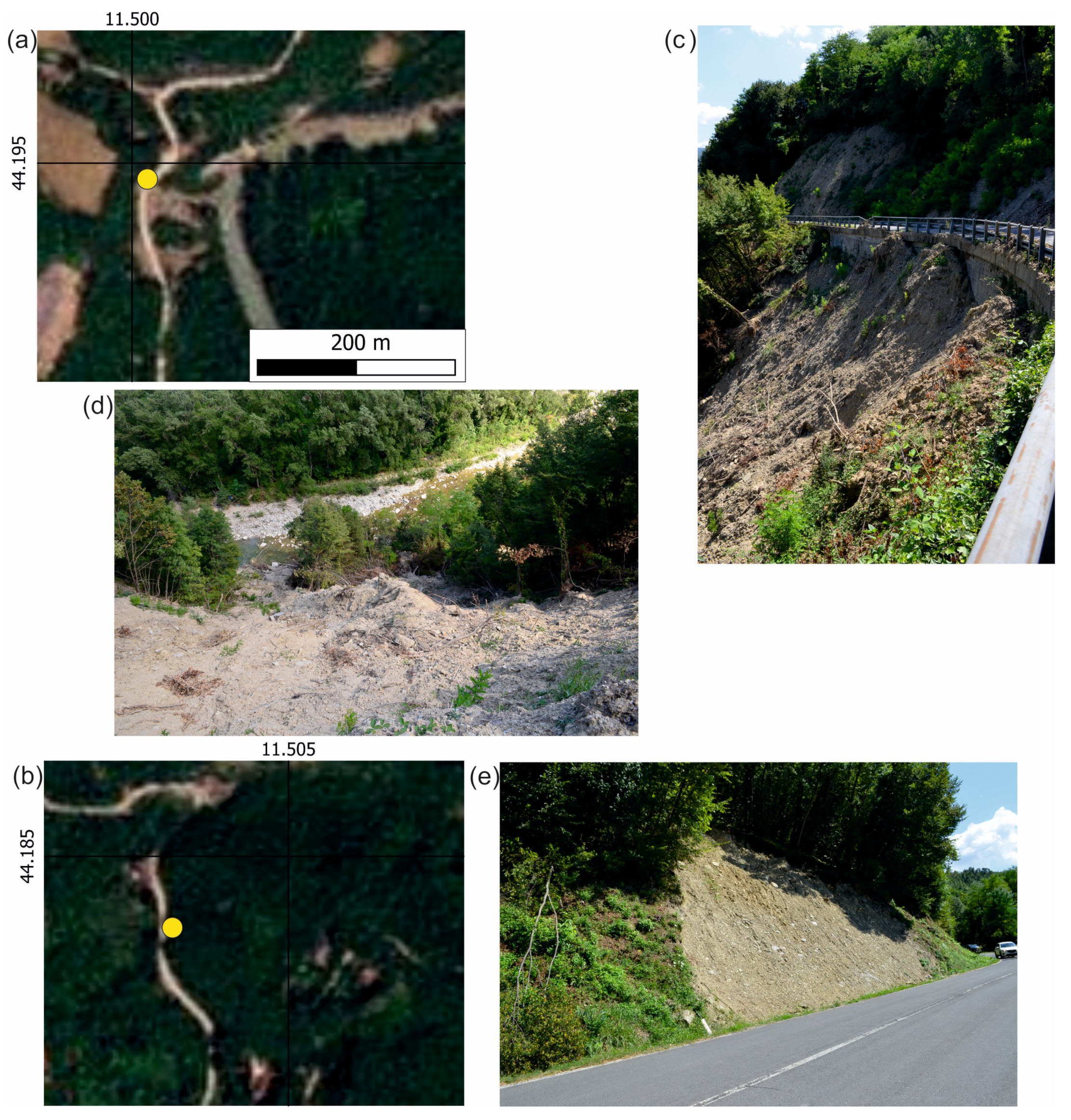
Figure 13.
Satellite images and field photographs of landslides impacting the road network along Province Road SP610 in the Castel del Rio Municipality: (a,b) Planet images acquired on 23 May, yellow dots are the locations where pictures were taken; (c,d) field photos of a landslide impacting the road, the deposit area lies in proximity of Santerno River; and (e) field photo of a smaller landslide, not recognizable on satellite imagery. All the photographs were shot by M. F. Ferrario on 30 July 2023.


Table 1.
Details on the rainfall gauges plotted in Figure 2.
Table 1.
Details on the rainfall gauges plotted in Figure 2.
| ID | Station | Municipality | Province | Elevation (m asl) | Longitude | Latitude | Hydrographic Basin |
|---|---|---|---|---|---|---|---|
| BTO | Borgo Tossignano | Borgo Tossignano | Bologna | 98 | 11.578993 | 44.27467 | Santerno |
| TAV | Le Taverne | Fontanelice | Bologna | 486 | 11.587499 | 44.2492 | Santerno |
| ALB | Monte Albano | Casola Valsenio | Ravenna | 480 | 11.6734246 | 44.22432 | Senio |
| PVE | Ponte Verucchio | Verucchio | Rimini | 116 | 12.405109 | 43.9829 | Marecchia |
| TRE | Trebbio | Modigliana | Forlì-Cesena | 570 | 11.8371627 | 44.13697 | Lamone |
| VER | Vergato | Vergato | Bologna | 193 | 11.113128 | 44.2878 | Reno |
Table 2.
Lithological classes.
| Lithology Class | Description |
|---|---|
| U1 | Competent massive or well-bedded rocks (mainly limestones and dolostones) |
| U2 | Siltstones, marls and limestones interbedded with marls |
| U3 | Sandstones and sandstones interbedded with marls and siltstones |
| U4 | Conglomerates and breccias |
| U5 | Gypsum (massive or breccia facies) |
Table 3.
Land use classes.
| Land Use Class | Description |
|---|---|
| L1 | Urban (residential and industrial) |
| L2 | Arable land |
| L3 | Agricultural (trees and vineyard) |
| L4 | Meadows |
| L5 | Woods (both evergreen and deciduous) |
| L6 | Bare rocks and badlands |
| L7 | Shrubs |
| L8 | Water (lakes, rivers and swamps) |
Table 4.
Summary of the considered classes as possible predisposing factors and calculated InfoVAL index (Wi).
Table 4.
Summary of the considered classes as possible predisposing factors and calculated InfoVAL index (Wi).
| Predictor | Class | InfoVAL Index (Wi) |
|---|---|---|
| Lithology | U1: Competent massive or well-bedded rocks (mainly limestones and dolostones) | 0.09 |
| U2: Siltstones, marls and limestones interbedded with marls | 0.14 | |
| U3: Sandstones and sandstones interbedded with marls and siltstones | −0.41 | |
| U4: Conglomerates and breccias | −0.48 | |
| U5: Gypsum (massive or breccia facies) | 0.08 | |
| Land use | L1: Urban (residential and industrial) | −1.60 |
| L2: Arable land | −0.67 | |
| L3: Agricultural (trees and shrubs) | −0.53 | |
| L4: Meadows | −0.23 | |
| L5: Woods (both evergreen and deciduous) | 0.56 | |
| L6: Bare rock and badlands | 1.57 | |
| L7: Shrubs | 0.45 | |
| L8: Water (lakes, rivers and swamps) | 0.22 | |
| Slope (°) | 0–10 | −0.31 |
| 10–20 | 0.13 | |
| 20–30 | 0.62 | |
| 30–40 | 0.71 | |
| 40–50 | 0.60 | |
| 50–60 | 0.44 | |
| 60–70 | 0.79 | |
| 70–80 | 2.16 | |
| 80–90 | - | |
| Distance from roads (m) | 0–200 | −0.07 |
| 200–400 | 0.46 | |
| 400–600 | 0.56 | |
| 600–800 | 0.40 | |
| 800–1000 | 0.19 | |
| 1000–1200 | −0.24 | |
| 1200–1400 | −0.81 | |
| 1400–1600 | −0.46 | |
| 1600–1800 | −0.70 | |
| 1800–2000 | −0.14 |
Disclaimer/Publisher’s Note: The statements, opinions and data contained in all publications are solely those of the individual author(s) and contributor(s) and not of MDPI and/or the editor(s). MDPI and/or the editor(s) disclaim responsibility for any injury to people or property resulting from any ideas, methods, instructions or products referred to in the content. |
© 2023 by the authors. Licensee MDPI, Basel, Switzerland. This article is an open access article distributed under the terms and conditions of the Creative Commons Attribution (CC BY) license (https://creativecommons.org/licenses/by/4.0/).
Share and Cite
MDPI and ACS Style
Ferrario, M.F.; Livio, F. Rapid Mapping of Landslides Induced by Heavy Rainfall in the Emilia-Romagna (Italy) Region in May 2023. Remote Sens. 2024, 16, 122. https://doi.org/10.3390/rs16010122
AMA Style
Ferrario MF, Livio F. Rapid Mapping of Landslides Induced by Heavy Rainfall in the Emilia-Romagna (Italy) Region in May 2023. Remote Sensing. 2024; 16(1):122. https://doi.org/10.3390/rs16010122
Chicago/Turabian StyleFerrario, Maria Francesca, and Franz Livio. 2024. "Rapid Mapping of Landslides Induced by Heavy Rainfall in the Emilia-Romagna (Italy) Region in May 2023" Remote Sensing 16, no. 1: 122. https://doi.org/10.3390/rs16010122
Note that from the first issue of 2016, this journal uses article numbers instead of page numbers. See further details here.