A Conceptual Model for Detecting Small-Scale Forest Disturbances Based on Ecosystem Morphological Traits

Abstract

Current LiDAR-based methods for detecting forest change use a host of statistically selected variables which typically lack a biological link with the characteristics of the ecosystem. Consensus of the literature indicates that many authors use LiDAR to derive ecosystem morphological traits (EMTs)—namely, vegetation height, vegetation cover, and vertical structural complexity—to identify small-scale changes in forest ecosystems. Here, we provide a conceptual, biological model for predicting forest aboveground biomass (AGB) change based on EMTs. We show that through use of a multitemporal dataset it is possible to not only identify losses caused by logging in the period between data collection but also identify regions of regrowth from prior logging using EMTs. This sensitivity to the change in forest dynamics was the criterion by which LiDAR metrics were selected as proxies for each EMT. For vegetation height, results showed that the top-of-canopy height derived from a canopy height model was more sensitive to logging than the average or high percentile of raw LiDAR height distributions. For vegetation cover metrics, lower height thresholds for fractional cover calculations were more sensitive to selective logging and the regeneration of understory. For describing the structural complexity in the vertical profile, the Gini coefficient was found to be superior to foliage height diversity for detecting the dynamics occurring over the years after logging. The subsequent conceptual model for AGB estimation obtained a level of accuracy which was comparable to a model that was statistically optimised for that same area. We argue that a widespread adoption of an EMT-based conceptual approach would improve the transferability and comparability of LiDAR models for AGB worldwide.

1. Introduction

Tropical forests are complex ecosystems which provide important ecosystem services, especially relating to global carbon and water cycles [1,2]. Tropical forests suffer from deforestation and illegal logging which have significant environmental, ecological, and economic impacts locally and globally [3,4]. Remote sensing technologies are becoming increasingly efficient at detecting large-scale disturbances [5]; however, small-scale clearance activities in the Amazon rainforest account for half of Brazil’s deforestation rate [6]. This small-scale degradation includes natural windfall and legal and illegal selective logging and is difficult to detect using most forms of remote sensing due to their effective resolutions [5]. There is therefore a need to further develop current remote sensing technologies into methods that are more sensitive to such selective logging which would then be capable of detecting and monitoring the degradation.

Ecosystem morphological traits (EMTs)—namely, vegetation height, vegetation cover, and vertical structural complexity—are a proposed framework of “ecosystem-agnostic” variables, which can be derived from a suite of three-dimensional (3D) remote sensing methods, to comprehensively describe the structural properties of a range of diverse ecosystem environments [7,8,9,10]. Ecosystem disturbance, such as selective logging in tropical forests, can cause changes in any of these EMTs [11], and therefore each of these EMTs may be independently relevant to monitor in order to effectively fight tropical forest degradation. Efforts to detect forest degradation have most commonly been based on the detection of changes in either forest cover only [5] or forest height only [12]. These approaches may miss selective logging activities concentrating on small trees underneath the upper canopy. There is thus a need to develop methods which can identify degradation from changes in any of these EMTs, and not simply based on the loss of either forest cover or vegetation height.

Since remote sensing methods are best suited to tackle large-scale disturbance [5], monitoring and mapping of small-scale selective logging in tropical forests are still heavily reliant upon expensive and time-consuming field survey techniques [13]. Among the multiple techniques that can be used to combat degradation, airborne LiDAR—one type of 3D remote sensing [10]—has undergone widespread use due to its capacity to reliably measure detailed characteristics of forest ecosystems at very high spatial resolutions [14,15,16,17,18]. In addition to reliable and accurate data collection, the use of airborne LiDAR benefits from fast and affordable large-scale estimation, which allows one to detect logging activities and subsequent biomass changes over large and inaccessible landscapes [19,20].

Models using data from airborne LiDAR can be used to generate maps of aboveground biomass (AGB) estimates over large areas [16,17,18,21,22,23,24,25,26,27,28,29,30,31,32]. Multitemporal LiDAR can be used to evaluate small-scale changes [33,34] but the capacity of these maps to detect small-scale changes is contingent upon AGB estimation models being accurate enough to detect forest disturbance [35]. The selection of predictor variables for AGB estimation models from LiDAR follows two fundamentally distinctive approaches: data-driven methods employing a statistical criterion that delivers an ad hoc selection of variables (referred to as “statistical models” hereafter), or conceptual approaches driven by knowledge of biological relationships that aim to obtain generalisable models of global validity (referred to as “conceptual models” hereafter). Statistical models are based on the selecting predictors under a given criterion tested over a given sample, such as statistical significance [15,33,35], information criteria [36], penalised likelihood [37], maximisation of accuracy [21,30], or algorithms combining several criteria [38]. These models only work ad hoc, and potential issues have been identified, such as tendencies to overfit to their sample and lack of transferability [39,40,41]. By contrast, conceptual models employ variables that are decided beforehand because they are known to have biological and physical relationships with forest AGB [22,41]. We argue that modelling forest AGB should be based on EMTs, and thus an investigation on LiDAR proxies identified for each of them can help identify forest AGB changes from small-scale logging.

The current paradigm shift around airborne LiDAR remote sensing is that EMTs may be better measured directly using airborne LiDAR than by other methods, including ground assessments [42]. Thus, airborne LiDAR could ultimately “ground truth” other data sources and serve as a reference to combine different data sources [27]. However, there is still a lack of consensus as to which exact airborne LiDAR proxies (a.k.a., LiDAR metrics, sensu. Naesset, 2002) would most suitably correspond to each of the EMTs: height, cover, and complexity [10]. For this reason, in this study we focus on identifying the LiDAR proxies for each EMT on the basis of their sensitivity to small-scale disturbances (e.g., Nunes et al., 2021) rather than on the estimated AGB change itself (e.g., Rex et al., 2020). The expected behaviours of each of the EMTs in response to small-scale disturbance are outlined below (Figure 1). For each EMT there is a range of proxies that are commonly employed by authors in AGB modelling (

Table 1. Ecosystem morphological traits, their associated metrics, and examples of their use.

EMT	Metrics		References
Vegetation height	TCH		Lefsky et al., 1999 [43]; Asner and Mascaro, 2014 [22]; Fahey et al., 2019 [9]; Almeida et al., 2019 [27]; Silva et al., 2019 [44]
	MEANH		Næsset et al., 2002 [15]; Hinsley et al., 2009 [45]; Kane et al., 2010 [46]; Zellweger et al., 2016 [47]; Fahey et al., 2019 [9]; Rex et al., 2020 [33]
	MODEH		Næsset et al., 2002 [15]; Fahey et al., 2019 [9]; Rex et al., 2020 [33]
	MEDIANH		Næsset et al., 2002 [15]; Rex et al., 2020 [33]
	Percentiles of height (H95, H75 etc.)		Næsset et al., 2002 [15]; Kane et al., 2010 [46]; Bater et al., 2011 [48]; Zellweger et al., 2016 [47]
Vegetation cover	Leaf area index/plant area index	COVER2 COVER5 COVER10 COVER20	Nelson et al., 1988 [49]; Næsset et al., 2002 [15]; Morsdorf et al., 2006 [50]; Solberg, 2010 [51]; Korhonen et al., 2011 [52]; Görgens et al. 2017 [53]; Schneider et al., 2017 [8]
	Gap fraction		Wedeux & Coomes, 2015 [54]; Jucker et al., 2018; Silva et al., 2019 [44]
Structural complexity of vegetation	Entropy	FHD	Clawges et al., 2008 [55]; Bergen et al., 2009 [56]; Valbuena et al. 2012 [57]; Zellweger et al., 2016 [47]; Schneider et al., 2017 [8]
	Variability	SD	Kane et al., 2010 [46]; Bouvier et al., 2015 [41]; Coops et al., 2016 [7]; Zellweger et al., 2016 [47]
		GC	Kane et al., 2010 [46]; Valbuena et al., 2013; 2017b; 2020 [10,39,58]; Adnan et al., 2021 [31]

).

We evaluated the suitability of EMTs—namely vegetation height, cover, and structural complexity—for monitoring selectively logged forests through use of LiDAR proxies. Specifically, we evaluated the temporal dynamics of LiDAR-derived metrics after selective logging activities, assessing which of these metrics were more sensitive to logging. We also assessed the capacity of the metrics to identify historical logging which preceded LiDAR survey through detection of additional growth in multitemporal datasets. These analyses permitted us to identify the LiDAR proxies for each of the three EMTs most sensitive to small-scale selective logging. In turn, this allowed us to develop a conceptual model for AGB estimation using EMTs to produce the most suitable LiDAR model both in terms of its accuracy and its capacity to describe the overall variability in AGB. We compared this model to an established model with the intent of illustrating the relative accuracy of the new model when compared to that of a commonly used alternative. The advantage of our EMT-based conceptual model is that the traits have a mechanistic link with the characteristics of the ecosystem rather than being selected via machine learning and statistical analyses. Through use of this conceptual approach, we set out to show that there are alternative means of variable selection available other than the use of automatic selection methods such as AIC.

2. Materials and Methods

2.1. Study Area

We assessed the data from the Fazenda Cauaxi in Pará state, Brazil. The region is humid and tropical with the average total precipitation annually being 2200 mm and with predominantly flat topology and an elevation ranging between 74 and 150 m above sea level [32]. The primary form of vegetation in the region is ombrophilous dense forest with the upper canopy having a mean height between 30 and 40 m and emergent trees reaching above the canopy up to 50 m tall [20,32]. The site consisted of a region split into 12 blocks of 100 ha which were either left unlogged or were subject to selective logging by similar methods at different times in the years 2006–2013 [59]. Previous works in this same area have carried out assessments of the following: forest types at different stages of degradation [25], the impact of LiDAR pulse density on the accuracy of AGB estimations [60], identification of logging damage impacts and recovery [59], and the development of an improved framework for reduced impact logging [61]. Previous AGB models from LiDAR in this study area were “statistical models” using either machine learning or statistical approaches for variable selection [25,33,38,59,60,62].

2.2. Field Data

The field dataset was collected in 2014 from 85 plots of 50 × 50 m (0.25 ha) with 100 m spacing along transects through logged regions of the study area. Plot corners were registered using differential GNSS (GeoXH6000, Trimble Navigation, Ltd.; Dayton, OH, USA). Along one side of each plot a subplot of 5 × 50 m (250 m²) was marked out. At each plot, trees with a diameter at 1.3 m breast height (dbh; cm) greater than or equal to 35 cm were measured within the entirety of the larger plot, whereas trees with dbh 35–10 cm were measured exclusively within the 250 m² subplot. AGB estimates for each field data plot were aggregated from the AGB estimated for each tree using the widely adopted allometric model by Chave et al. (2014) [63]. The value for environmental stress parameter (E) used in the model was E = −0.104 for the entire study site as in Rex et al. (2020) which used the same field dataset.

2.3. LiDAR Data Acquisition and Processing

LiDAR datasets were collected by a joint venture of the Brazilian Corporation of Agricultural Research (EMBRAPA) and the United States Forest Service (USFS), called “Sustainable Landscapes Brazil”. Collection took place in 2012, 2014, and 2017, at a flight altitude of 850 m and overlaps of 65–70%; further details regarding LiDAR data collection such as sensor attributes and flight details are available in

Table 2. Statistics reflecting accuracy and goodness of fit for AGB models.

		Adj.R2	RMSE (Mg/ha)	RMSE (%)	MD (Mg/ha)	MD (%)	SSR	SDR
Height	a * × TCH *	0.82	49.93	20.97	1.64	0.69	1.03	0.88
	MEANH *	0.82	50.66	21.28	−7.89	3.31	1.01	0.69
	H95 *	0.60	69.54	29.20	−11.24	−4.72	1.01	0.58
	a * × H75 *	0.56	56.73	23.83	1.02	0.43	0.91	0.76
Cover	COVER2 *	0.01	87.77	36.86	−15.84	−6.65	1.03	0.10
	COVER5 *	0.21	85.67	35.98	−15.53	−6.52	1.04	0.15
	a * × COVER10 *	0.50	74.72	31.38	1.41	0.59	1.02	0.52
	COVER20 *	0.75	57.54	24.16	−5.85	−2.46	1.01	0.75
Structural Complexity	a * × GC *	0.13	80.79	33.93	1.92	0.81	1.02	0.46
	a * × FHD *	0.37	70.31	29.53	2.64	1.11	1.05	0.80
	a * × SD *	0.07	83.06	34.88	1.62	0.68	1.03	0.32
Bi-variate models
TCH * × COVER2 *		0.82	50.07	21.03	−5.47	−2.30	1.03	0.83
TCH * × COVER5 *		0.81	50.96	21.40	−6.15	−2.58	1.03	0.80
TCH * × COVER10 *		0.80	52.95	22.24	−7.79	−3.27	1.03	0.72
TCH * × COVER20 *		0.80	54.73	22.98	−8.66	−3.64	1.03	0.62
Tri-variate models
TCH * × COVER2 * × GC *		0.81	50.46	21.19	−4.52	−1.90	1.05	0.87
TCH * × COVER2 * × SD *		0.81	51.17	21.49	−4.71	−1.98	1.05	0.86

* Denotes variable is significant (p < 0.05), a = 1 if not shown, only significant models shown.

of Rex et al. (2020). Processing of LiDAR data was conducted using the software FUSION/LDV version 3.8 [64], LAStools [65], and the LidR package in R [66].

Initially, the data were classified to identify ground returns and then the elevation values for returns were normalised to heights-above-ground (Figure 2). The pulse densities were not standardised across the LiDAR data collection, as it was shown that for plot level AGB predictions there is no significant impact to the accuracy when the pulse density is above the range of 1.0 pulses·m⁻² [60].

Of the metrics listed in Table 1, not all were selected in this study as candidates for EMT proxies. MEANH, H75, and H95 were calculated directly from the point cloud. TCH was calculated as the mean of the CHM values aggregated at the grid resolution of 50 m. The cover was calculated at a range of height thresholds: 2, 5, 10, and 20 m above the ground (COVER2, COVER5, COVER10, and COVER20, respectively). FHD was calculated based upon Shannon’s diversity [67] abundances being the proportions of LiDAR returns within six contiguous strata along the vertical profile: <2, 2–5, 5–10, 10–20, 20–30, >30 m above the ground. GC was calculated as half of the relative mean absolute difference [39]. Unless otherwise specified, the LiDAR-derived metrics were available from the outputs of functions in FUSION, and they were calculated for the LiDAR returns at the position of the field plots and throughout the entire study area using a grid of 50 m spatial resolution, resulting in one complete grid for each of the collection years. A canopy height model (CHM) was generated at 1 m spatial resolution using the grid_canopy function available in LidR.

The maps of percentage change in LiDAR-derived metrics were generated using the raster package in R [68] and the software QGIS [69]. To produce graphs of temporal dynamics for each metric, we calculated the number of complete years since logging which was then subsequently used as the variable expressing the temporal dimension. Since metrics were expressed in different units and had disparate variances, we used normalised z-scores to fairly compare the changes observed at different metrics. The normalised z-scores of each metric were plotted against the years since logging using the R package ggplot2 [70], showing the mean of all the corresponding 50 × 50 m cells of the grid along with ribbons showing their 95% confidence intervals.

2.4. AGB Modelling

The dataset used for the development of models consisted of the plot aggregate AGB estimations from the field data and the 2014 LiDAR metrics calculated at the location of those same plots. The power-law equation for the Asner et al. (2012) model (hereafter referred to as the “TCH model”) was:

$$AGB=a\times TC{H}^b$$

(1)

where AGB was the aboveground biomass in Mg/ha and TCH the top-of-canopy height in meters derived from LiDAR. The model parameters a and b were determined through the linearised log-log version of the model [12], including the correction for the intercept value when back-transforming the parameter a from the linear model [71].

Further from the TCH model which accounted for a vegetation height EMT only, we considered a conceptual model under the postulate that all the EMTs considered in Valbuena et al. (2020)—vegetation height, vegetation cover, and vertical structural complexity—explain an independent proportion of variability in AGB. Hereafter, we refer to this model as the “EMT model”, which has a similar power-law form that typically regulates these relationships [72,73,74] and is typically employed in LiDAR modelling [15]:

$$AGB=heigh{t}^{b1}\times cove{r}^{b2}\times complexit{y}^{b3}$$

(2)

where height was the value of the LiDAR metric chosen for vegetation height ETM (TCH being one of the candidates) in meters above the ground, cover was the value of the LiDAR metric chosen for vegetation cover in units between 0 and 1 expressing the proportion of area covered by vegetation above a chosen height threshold, and complexity is the value of the LiDAR metric chosen for the structural complexity trait. The units for expressing complexity are dependent upon the metric chosen, with the SD being expressed in meters, the GC ranging between 0 and 1, with GC = 0 denoting no height variability and GC = 1 denoting maximally variable, and FHD being a dimensionless measure ranging between FHD = 0 for an area with no vegetation and the logarithm of the number of strata used in its calculation which provides a value for maximum entropy (FHD = ln(6) = 1.79 in this case). Again, the model parameters a, b1, b2, and b3 were determined in the linearised log-log form of the model, including Baskerville’s correction for bias in the estimation of a [71].

To identify the metrics that would serve as the LiDAR proxies for the EMTs in the EMT model (Equation (2)), several means of variable selection were employed:

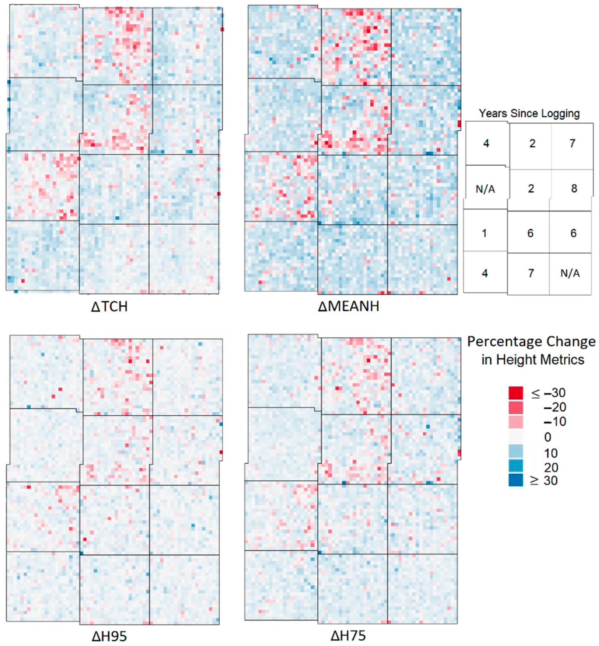
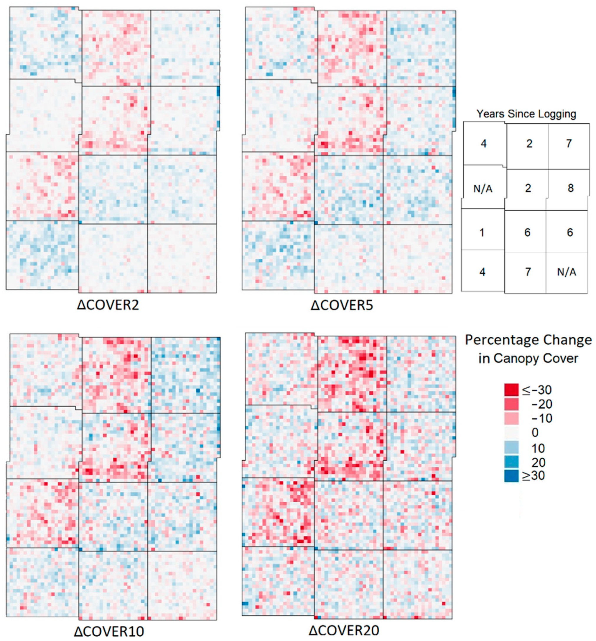
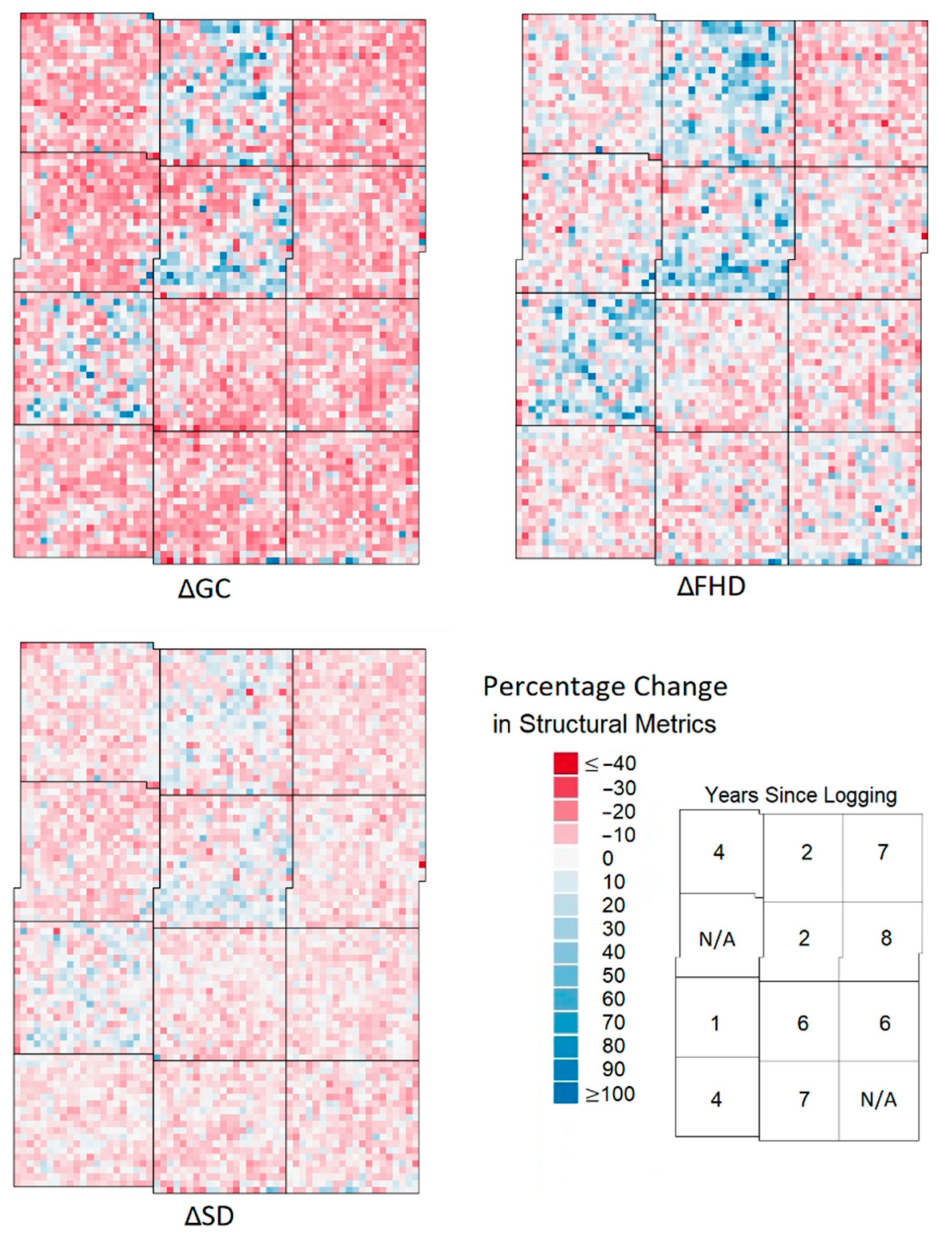
• Maps of percentage change in metrics (denoted as Δ in front of each metric). From the maps of change in the metrics it was possible to identify the metrics which showed the greatest percentage change in areas of recent and historical selective logging, and thus sensitivity to small-scale disturbance, and this was one factor that was used to select LiDAR proxies. One-tailed Wilcoxon rank tests, for data grouped by the logging year, were used to assess the significance of the increase or decrease in a given metric compared to the baseline defined by the unlogged areas.
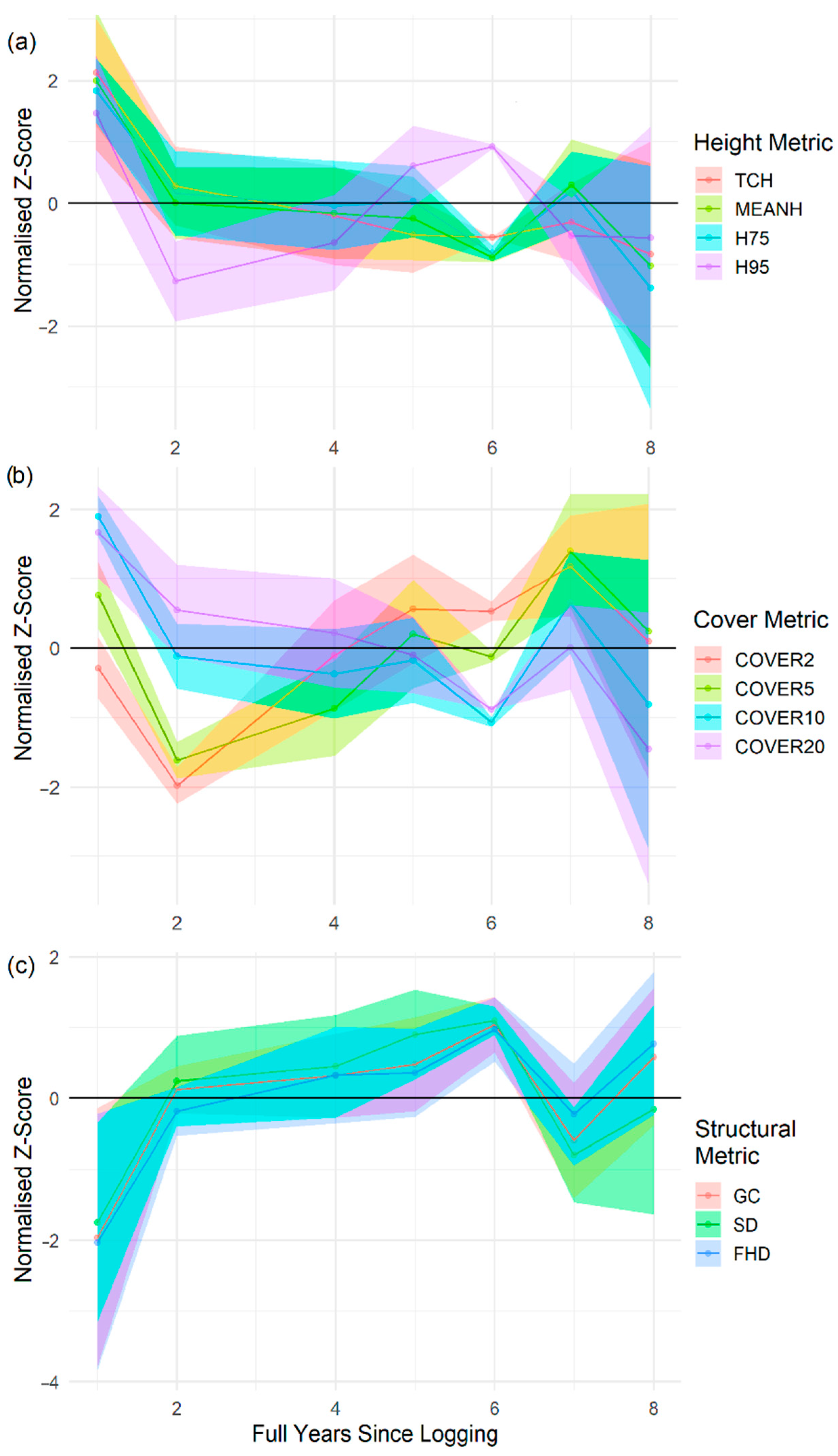
• Graphs of temporal dynamics of metrics in the years following logging. The graphs of normalised z-scores (in which the mean is equal to 0) were used to identify which metrics showed the greatest change in the years after selective logging and the graphs also highlighted how long it took metrics to stabilise and thus for how long after logging metrics were sensitive to the impacts of small-scale disturbance.
• Correlation plots and Pearson correlation coefficients. Plots of the correlation of change in metrics, with trendlines and inset correlation values. These identified relationships between metrics that allowed for informed decisions to be made with regards to the use of metrics which may explain the same variance.

Final selection of the metrics which were used as variables in the EMT model was achieved through comparison of the information derived from the above methods of variable selection and information from accuracy assessments of predictive models using the different metrics to identify the metrics which are most sensitive to small-scale disturbance.

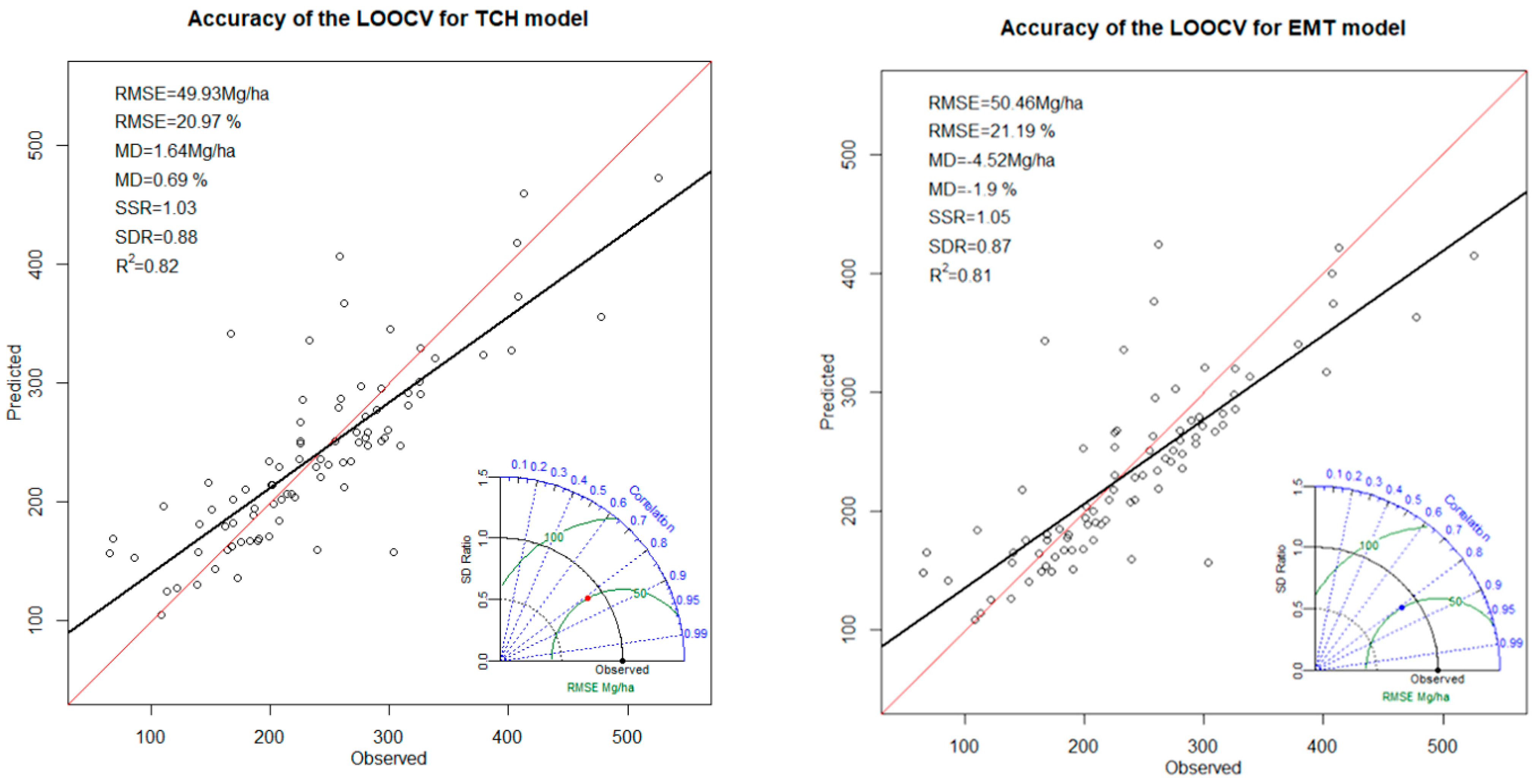
2.5. Accuracy Assessment

Leave-one-out cross-validation (LOOCV) was carried out to assess the predictions of the two models. This is performed through the iterative removal of one case (i) from the total n, with the remaining used to calculate a new AGB prediction for the absence of that case ($pre{d}_i^{cv}$). For the purposes of notation, superscript “cv” identifies calculations after the cross-validation procedure, as opposed to superscript “fit” which denotes non-cross-validated measures. We employed five analytical measures and two graphical methods for accuracy diagnosis. The analytical measures were employed to evaluate:

(1)

The precision of predictions given as the absolute and relative root mean squared error (RMSE) of predictions against the observed:

$$RMSE=S{S}^{cv}/n$$

(3)

where $S{S}^{cv}$ was the predicted sum of squares through LOOCV:

$$S{S}^{cv}={{\displaystyle \sum }_{i=1}^n\left(pre{d}_i^{cv}-ob{s}_i\right)}^2$$

(4)

The error in RMSE was given in AGB units, and also the relative error RMSE% as the coefficient of variation of RMSE, i.e., calculated by dividing it by the mean observed AGB ($\overline{obs}$).

(2)

The degree of under- or over-prediction as the mean difference (MD) of the predictions minus the observed:

$$MD={\displaystyle \sum }_{i=1}^n\frac{\left(pre{d}_i^{cv}-ob{s}_i\right)}{n}$$

(5)

Likewise, MD was presented both in AGB units and relative mean difference (MD%) calculated by dividing it by $\overline{obs}$.

(3)

The agreement between observed and predicted, evaluated by the coefficient of determination $R^2$ (Valbuena et al., 2019):

$$R^2=1-S{S}^{cv}/S{S}_{obs}^{tot}$$

(6)

where $S{S}_{obs}^{tot}$ was the sum of squared differences of each observation from $\overline{obs}$:

$$S{S}_{obs}^{tot}={{\displaystyle \sum }_{i=1}^n\left(ob{s}_i-\overline{obs}\right)}^2$$

(7)

Another measure of agreement depicted in Taylor diagrams (see below) was Pearson’s correlation (r), but we discarded its analytical use since Valbuena et al. (2019) showed $R^2$ to more faithfully represent the agreement between observed and predicted.

(4)

The degree of overfitting, comparing the sums of squares obtained with (“cv”) and without (“fit”) cross-validation (Valbuena et al. 2017), calculated as the sum of squares ratio (SSR):

$$SSR=\sqrt{S{S}^{cv}}/\sqrt{S{S}^{fit}}$$

(8)

where $S{S}^{fit}$ was the predicted sum of squares without LOOCV:

$$S{S}^{fit}={{\displaystyle \sum }_{i=1}^n\left(pre{d}_i^{fit}-ob{s}_i\right)}^2$$

(9)

SSR provides a suitable measure of increase in the unexplained variance when carrying out the LOOCV. It has been suggested that the difference between model fit and cross-validation exceeding 10% (i.e., SSR = 0.90–1.10) signals a model that is overfitted to the sample [39,75].

(5)

The model’s capacity to match the AGB variability originally observed. As the standard deviation ratio (SDR):

$$SDR=\sqrt{S{S}_{pre}^{tot}}/\sqrt{S{S}_{obs}^{tot}}$$

(10)

where $S{S}_{pre}^{tot}$ was the sum of squared differences of each observation from the mean predicted AGB ($\overline{pre}$):

$$S{S}_{pre}^{tot}={{\displaystyle \sum }_{i=1}^n\left(pr{e}_i-\overline{pre}\right)}^2$$

(11)

Moreover, the graphical methods employed for accuracy assessment were:

Observed versus predicted plots depicting the LOOCV predictions. The plots include both the 1:1 line and their regression, which can be tested against the null hypothesis of alpha = 0 and beta = 1 [18], on the basis that predicted is x and observed y in that regression analysis [76].

Taylor diagrams. A prerequisite for AGB models to produce reliable maps (particularly to detect small-scale changes) is to ensure that they not only predict the average AGB but the observed variability in AGB as well. To that end, we produced Taylor diagrams [77] for each of the LOOCV models using the taylor.diagram function of the package plotrix [78] which was then modified to normalise standard deviation without normalising RMSE and, for additional clarity of interpretation, through colour coding. Overfitting makes models less transferable by being overly specific to a single site and/or dataset, whereas the intent with the conceptual EMT model is to have a widely usable alternative to statistically driven, site-specific models and thus it may allow for the interpretation of the fitted model parameters in terms of their physical meaning. Taylor diagrams are a method of summarising multiple aspects of model performance in a single diagram. Three statistics are plotted on Taylor diagrams:

(a)

Correlation, denoted by the azimuthal angle (blue radial dashed lines and arc) which represents the Pearson correlation coefficient, evaluating similarity in patterns of distribution of the predicted and observed, which is also a measure of the similarity of the means. The Pearson correlation coefficient is a normalised measure of the linear correlation between two datasets, in this case the predictions of a leave-one-out model and the observed dataset [79]. Valbuena et al. (2019) [80] pointed out that only the squared correlation gives values comparable to the coefficient of determination in Equation (3), but correlation is added here as implemented in the package stats.

(b)

RMSE, proportional to the distance of a point from the reference for observed data, on the x-axis (which is shown by green arcs).

(c)

The standard deviation ratio of the cross-validation predictions to the observed is proportional to the radial distance from the origin (black arcs). The standard deviation ratio reflects how well the predictions reflect the variance of observed data.

3. Results

3.1. Vegetation Height

The maps of the percentage change in LiDAR-derived height metrics (Figure 3—ΔTCH, ΔMEANH, ΔH75, and ΔH95) show that all the height metrics highlight areas of logging in the years between the 2012 and 2014 data collection. The areas of greatest decrease in height metrics were the areas which were selectively logged in 2012 and 2013 (significant decrease in all metrics, p < 0.01). This can be seen from the example transect (Figure 3). For TCH and H75 it was even possible to detect the older logging activities that occurred before 2012 from anomalously greater increases compared to the baseline growth in unlogged areas (significant increases, p < 0.01). Other common metrics like MEANH or H95 could not detect this anomalous growth (non-significant increase, p > 0.05).

The graph of the temporal dynamics of height metrics (Figure 4a) shows that H95 had the greatest decrease in the years immediately following logging. However, it also shows an erratic upward trend four years after logging, which may be an indication of lack of robustness in this metric. Considering this in addition to the lower sensitivity shown in the maps of change for H95, this may be an indication that H95 is not the most suitable LiDAR proxy for vegetation height. Of the other three metrics, H75 also showed low sensitivity in the maps and thus the dynamics in the years after selective logging were quite similar, indicated by their overlapping confidence ribbons. MEANH and TCH appeared to be the most sensitive to logging, which can make them the most suitable metrics to select as LiDAR proxy for vegetation height.

Univariate models of AGB estimation were produced for each of the height metrics to assess their relationship to AGB. Their respective RMSEs (Table 2) showed that the model accuracy was greatest for TCH. The SDRs also demonstrated that TCH can best model the range of variability in the area, with the TCH-based model predicting 88% of the total standard deviation in AGB. SSR results show that none of the models were overfitted to the sample, with cross-validated values deviating less than 10% from model residuals, although the MD of H95 showed a tendency for higher bias than other metrics. Based on these model results, the results of the graph of temporal dynamics, and the maps, it is unclear which of TCH or MEANH would be the most suitable LiDAR proxy for vegetation height. We will use TCH as the LiDAR proxy as it is derived directly from the point cloud data.

3.2. Vegetation Cover

The maps of percentage change in LiDAR-derived cover metrics (Figure 5—ΔCOVER2, ΔCOVER5, ΔCOVER10, and ΔCOVER20) clearly identify the regions that were logged in 2012 and 2013 (significant decreases, p < 0.01). In blocks from earlier logging activities (2006–2010), ΔCOVER2, ΔCOVER5, and ΔCOVER10 highlight different stages of regrowth (significant increases, p < 0.01). On the other hand, this regrowth cannot be identified from ΔCOVER20 (non-significant increase, p > 0.05).

The temporal dynamics of the cover metrics (Figure 4b) show that the most significant decrease in the years following logging can be detected using COVER2. Additionally, COVER2 takes more years to stabilise than the metrics with greater height thresholds, giving potential to detect changes in cover for more years after logging. These results suggest that lower height thresholds are more sensitive to reduced impact logging and subsequently may therefore contribute to more accurate estimation of AGB if used as one of the morphological traits in calculations.

Univariate models of cover (Table 2) to predict AGB show a trend of RMSE falling and SDR increasing as the cover threshold height increases, thus accuracy increases with the cover. By contrast, when cover is modelled together with TCH (Table 2, bivariate models) the trends in the values of RMSE and SDR reverse, and the lower height thresholds performed better. Based on the maps, the graph of temporal dynamics, and the accuracy results of the bivariate models, COVER2 is the clear choice of LiDAR proxy for the vegetation cover EMT.

3.3. Structural Complexity

The maps of percentage change in the structural metrics (Figure 6—ΔGC, ΔFHD, and ΔSD) display distinct areas of increased structural complexity for all structural metrics in the blocks that were logged between 2012 and 2014 (significant increases, p < 0.01). ΔGC and ΔFHD highlight decreases in structural complexity in the regions that were logged prior to LiDAR data collection as the regions regrow (significant decreases, p < 0.01); by contrast, SD does not describe regions of regrowth from previous logging (non-significant decrease, p > 0.05).

The graph of temporal dynamics of structural complexity metrics after selective logging (Figure 4c) shows that all the structural complexity metrics are sensitive to selective logging. The temporal dynamics of all three metrics are quite similar, with sharp increases in the years after logging before beginning to stabilise, and the confidence ribbons of all metrics overlap substantially.

Accuracy assessment of the single-variable models of AGB estimation for each of the structural complexity metrics (Table 2) shows that FHD performs best with the highest explained variance (SDR) and lowest RMSE. Accuracy assessment of three-variable models of the same structure as that proposed for the final EMT model (Table 2) found that FHD yielded an insignificant model and, in further contrast to the univariate models, the trivariate models with GC and SD perform similarly to each other. GC will be selected as the LiDAR proxy for structural complexity, given the similar performance of GC to SD in the trivariate models and the prospect that GC could significantly detect the changes in structural complexity from the logging in 2006–2010.

3.4. TCH Model versus EMT Model

The chosen LiDAR proxies for the EMT model were TCH, COVER2, and GC. The EMT model was compared to the TCH model and the results of the accuracy assessment show that the TCH model and the EMT model were able to predict AGB with very similar levels of accuracy. From the observed vs. leave-one-out prediction plots (Figure 7) there appears to be a very high level of correlation between the AGB values derived from field plot observations and the leave-one-out predictions of the two models. The plots for the two models show that both models fail to quite capture the variance of the observed data, as they over predict low values and under predict high values, but they do have relatively small values for RMSE and mean difference, with the EMT model performing slightly better.

The inset Taylor diagrams show the RMSE values of the two models and they also show that the variance of the predictions of both models is not quite as great as the observed data, with both models showing an SDR of 0.88, thus only % of the variance of the observed data is explained. The Taylor diagram also gives a measure of the correlation that is seen between the predictions and the observations, the Pearson correlation coefficient, which for both models is approximately 0.8.

The plotted predictions of the LOOCV analyses show very similar relationships to the predictions of the full models, which suggests that neither model suffered from significant overfitting. This is corroborated by the SSR values, which show that neither model shows significant overfitting, though the EMT model may be more overfitted than the TCH model.

4. Discussion

Detection of logging continues to be a challenge and the development of new methods and models which can identify small-scale forest disturbance, particularly in the understory, is of great importance. Selective logging is even harder to detect than equivalent area of clear felling as the disturbance is spread out and thus the localised impacts are significantly reduced. As a result, methods of AGB calculation and detection of large-scale forest disturbance are potentially stretched to the limits of their sensitivity. More sensitive methods which could identify such selective logging practices are still in an early stage of development [81]; hence, in this study we have identified and proposed a conceptual modelling approach which may detect small-scale forest disturbances more accurately.

A standardised framework of essential biodiversity variables could be used to model ecosystems from a range of 3D-imaging remote sensing data sources [10]. This framework is the basis of the conceptual model in this study with terms for the ecosystem morphological traits of vegetation height, vegetation cover, and vertical structural complexity. The model developed using this method, the “EMT model”, was compared to a traditional method of AGB modelling presented in Asner and Mascaro (2014) and Coomes et al. (2017), the “TCH model”, a univariate model based upon TCH, which is a descriptor of ecosystem height. The TCH model does not account for variation in density of cover nor for a non-uniform ecosystem structure, which is not thought to be a limitation of the model in undisturbed ecosystems replete with old growth and consistently high cover but could be so in regions of small-scale disturbance.

Trait selection for the EMT model was based on maps of percentage change of metrics, normalised graphs of temporal dynamics of metrics, and the results of accuracy assessments of models using those metrics. The chosen LiDAR proxies to represent the traits in the EMT model were TCH, COVER2, and GC. Developing models for AGB estimation can sometimes be very intensive computationally, relying heavily upon statistics and even machine learning [33,62,82] for metric selection. In this study, we made use of visualisations of the change in metrics to determine the suitability of a metric to be included in a model.

The visualisations of the temporal dynamics of metrics (Figure 4) support the conceptual theory of how EMTs were expected to behave over time in a forest stand subject to selective logging and a period of recovery (Figure 1). The behaviour of the height metrics over time (Figure 4a) reflects the expected initial decline and subsequent recovery over time; these changes would be expected to be reflected by the TCH and EMT models which include height as a parameter. However, the EMT model additionally includes parameters for cover and structural complexity, where the graphs of their behaviour are shown to behave differently to one another and to height. Structural complexity rapidly changes in the first years after logging before rapidly stabilising, whereas the cover metrics take longer to stabilise, especially at the lower height thresholds where the early regenerative growth is detected. EMTs are sensitive to changes in the stand structure in the years after selective logging and can even detect historical logging that predates the survey through changes in the stand structure as illustrated by the clear delineation of the 12 plots logged at different times in the maps of percentage change in cover metrics (Figure 5).

From the visualisations of the change in metrics, the selection of the height metric was not clear. The results of accuracy analysis of univariate models of height metrics, and the graphs of the temporal dynamics of metrics, show that both TCH and MEANH perform similarly to one another and are more sensitive than H75 and H95. The maps of percentage change in the height metrics (Figure 1) were supplemented by additional one-tailed Wilcoxon rank tests to assess how the significance of the change in metrics for each logging year compared to the baseline of the unlogged areas. From the maps, it was again clear that the TCH and MEANH performed similarly and were more sensitive to selective logging than the other height metrics; however, the Wilcoxon rank tests showed that TCH had sensitivity to historical logging that was not seen in MEANH. Given the similarity in results and the results of the Wilcoxon, either metric could have made a suitable LiDAR proxy for height EMT. It was decided that TCH would be selected as LiDAR proxy despite it being generated from a CHM rather than directly from the point cloud. Asner and Mascaro (2014) suggested that the top of canopy height (TCH; [43]) could be a simple proxy for vegetation height universally linked to forest AGB and, although the derivation of CHMs involves additional processing, the use of CHMs provides a common processing milestone across sensors and platforms of 3D remote sensing [83], which enables their robust intercomparability and combination [10].

COVER2 was the standout metric for the cover EMT, which was an interesting outcome, as in other works that have made use of cover metrics in their predictive models, higher height thresholds were often the norm for cover metrics. Jucker et al. (2018) used gap fraction, which they calculated at 20 m above ground level. COVER20 was included in this study and it was found to be significantly less sensitive to selective logging than lower height thresholds and the sensitivity to selective logging appears to vary inversely with the height of the height threshold for the cover calculation. The result was not entirely unexpected as Kent et al. (2015) [84] showed that it was possible to identify regions of selectively logged forest in the advanced stages of recovery due to an elevated number of gaps which penetrated to the forest floor, as determined by gaps in vegetation at a height of 2 m using LiDAR data.

The chosen structural complexity term was GC which describes skewness of the forest structure, with low values representing uniformity of the heights of trees and high values representing an approach to bimodality. The relationship of GC and forest structural types is explored in greater depth by Valbuena et al. (2014) [84]. It should be noted that only the structural metrics describing variability yielded significant trivariate models, since FHD is a metric which describes entropy and was found to produce an insignificant trivariate model. SD was not chosen due to relative insensitivity to selective logging. In AGB models from LiDAR, the role of the structural complexity of vegetation is typically neglected, with few exceptions [31,41].

Direct comparison of the two models, the conceptually derived EMT model and the TCH model, shows that they performed similarly at estimating AGB; however, the differences between the models may be understated due to the fraction of plots in areas subject to selective logging being small. Consequently, most plots were not subject to disturbance; thus, the benefits of the logging-sensitive metrics of the EMT model were irrelevant and the overall improvement to modelling accuracy may have been underestimated.

Accuracy assessment of the two models found that the Asner and EMT models had very similar levels of accuracy; the explained variance, MD, and RMSE for the two models were extremely similar. An argument could be made for this being a failure of the EMT model and the method of its development, as it has been shown in literature that with more variables, models are able to replicate the mean more accurately at the expense of variance [18], and thus by only being marginally more accurate than the TCH model, it indicates the model is flawed due to the less significant parameters. A rebuttal to this argument is that the overfitting analyses showed both models being slightly overfitted, to a very similar degree, and that both under predict variance by 12–13%. This similar degree of overfitting suggests that the additional terms of the EMT model have therefore fallen victim to the MD-variance trade-off. The method of overfitting analysis used was LOOCV, which is known to yield lower MD and higher variance results than k-fold cross-validation. LOOCV was chosen, however, due to the sample size, and the results of the LOOCV were very similar to the fully fitted models for values of RMSE, MD, and variance, which suggests the effects of overfitting are small. If one is confident in using the existing TCH model, then similar confidence should be extended to the use of our proposed conceptual model outlined in this study. The proposed form of the EMT model, as found in this study, reflects a development of the TCH model in which the intercept, a, in Equation (1) is replaced by the terms for cover and structural complexity in Equation (2)—and thus the model becomes more informed by biological relationships.

5. Conclusions

The sensitivity of EMTs to the changes that happen in a selectively logged forest stand over time is evident, and this underlines the potential for a more biologically informed AGB estimation which makes use of EMTs. An EMT-based approach may be more suitable for the detection and quantification of illegal logging practices, but this remains to be seen. The use of EMTs for directly detecting changes in forest stands rather than AGB is demonstrated and represents a potential avenue for monitoring in addition to using those same EMTs for more monitoring through AGB modelling. Landscape scale methods of AGB estimation that are sensitive to selective logging will help prevent the over prediction of AGB stocks in regions where illegal logging takes place and may support monitoring of forests in selectively logged regions, particularly below the top of the canopy. Future use of EMTs in monitoring small-scale degradation through relative changes could allow for comparisons between ecosystems with vastly different AGB yields and encourage the use of more biologically informed metrics.

References

1. Brienen, R.J.; Phillips, O.L.; Feldpausch, T.R.; Gloor, E.; Baker, T.R.; Lloyd, J.; Lopez-Gonzalez, G.; Monteagudo-Mendoza, A.; Malhi, Y.; Lewis, S.L.; et al. Long-term decline of the Amazon carbon sink. Nature 2015, 519, 344–348. [Google Scholar] [CrossRef] [Green Version]
2. Phillips, O.L.; Brienen, R.J.W.; The RAINFOR Collaboration. Carbon uptake by mature Amazon forests has mitigated Amazon nations’ carbon emissions. Carbon Balance Manag. 2017, 12, 1. [Google Scholar] [CrossRef] [Green Version]
3. Reboredo, F. Socio-economic, environmental, and governance impacts of illegal logging. Environ. Syst. Decis. 2013, 33, 295–304. [Google Scholar] [CrossRef]
4. Condé, M.; Higuchi, N.; Adriano, J.N. Illegal Selective Logging and Forest Fires in the Northern Brazilian Amazon. Forests 2019, 10, 61. [Google Scholar] [CrossRef] [Green Version]
5. Gao, Y.; Skutsch, M.M.; Paneque-Gálvez, J.; Ghilardi, A. Remote sensing of forest degradation: A review. Environ. Res. Lett. 2020, 15, 103001. [Google Scholar] [CrossRef]
6. Assunção, J.; Gandour, C.; Rocha, R. DETERing Deforestation in the Amazon: Environmental Monitoring and Law Enforcement. Climate Policy Initiative, Núcleo de Avaliação de Políticas Climáticas, Pontifica Universidade Católica (PUC), Rio de Janeiro, 2017. p. 36. Available online: http://climatepolicyinitiative.org/wp-content/uploads/2013/05/DETERring-Deforestation-in-the-Brazilian-Amazon-Environmental-Monitoring-and-Law-Enforcement-Technical-Paper.pdf (accessed on 16 June 2021).
7. Coops, N.C.; Tompaski, P.; Nijland, W.; Rickbeil, G.J.; Nielsen, S.E.; Bater, C.W.; Stadt, J.J. A forest structure habitat index based on airborne laser scanning data. Ecol. Ind. 2016, 67, 346–357. [Google Scholar] [CrossRef]
8. Schneider, F.D.; Morsdorf, F.; Schmid, B.; Petchey, O.L.; Hueni, A.; Schimel, D.S.; Schaepman, M.E. Mapping functional diversity from remotely sensed morphological and physiological forest traits. Nat. Commun. 2017, 8, 1441. [Google Scholar] [CrossRef] [Green Version]
9. Fahey, R.T.; Atkins, J.W.; Gough, C.M.; Hardiman, B.S.; Nave, L.E.; Tallant, J.M.; Nadehoffer, K.J.; Vogel, C.; Scheuermann, C.M.; Stuart-Haëntjens, E.; et al. Defining a spectrum of integrative trait-based vegetation canopy structural types. Ecol. Lett. 2019, 22, 2049–2059. [Google Scholar] [CrossRef]
10. Valbuena, R.; O’Connor, B.; Zellweger, F.; Simonson, W.; Vihervaara, P.; Maltamo, M.; Silva, C.A.; Almeida, D.R.A.; Danks, F.; Morsdorf, F.; et al. Standardizing Ecosystem Morphological Traits from 3D Information Sources. Trends Ecol. Evol. 2020, 35, 656–667. [Google Scholar] [CrossRef]
11. Lefsky, M.A.; Hudak, A.T.; Cohen, W.B.; Acker, S.A. Patterns of covariance between forest stand and canopy structure in the Pacific Northwest. Remote. Sens. Environ. 2005, 95, 517–531. [Google Scholar] [CrossRef] [Green Version]
12. Asner, G.P.; Mascaro, J.; Muller-Landau, H.C.; Vieilledent, G.; Vaudry, R.; Rasamoelina, M.; Hall, J.S.; Van Breugel, M. A universal airborne LiDAR approach for tropical forest carbon mapping. Oecologia 2012, 168, 1147–1160. [Google Scholar] [CrossRef] [PubMed]
13. Locks, C.J.; Matricardi, E.A.T. Estimation of impacts of selective logging in the Amazon using LIDAR data. For. Sci. 2019, 29, 481–495. [Google Scholar] [CrossRef] [Green Version]
14. Lefsky, M.A.; Cohen, W.B.; Parker, G.G.; Harding, D.J. Lidar Remote Sensing for Ecosystem Studies: Lidar, an emerging remote sensing technology that directly measures the three-dimensional distribution of plant canopies, can accurately estimate vegetation structural attributes and should be of particular interest to forest, landscape, and global ecologists. BioScience 2002, 52, 19–30. [Google Scholar] [CrossRef]
15. Naesset, E. Predicting forest stand characteristics with airborne scanning laser using a practical two-stage procedure and field data. Remote. Sens. Environ. 2002, 80, 88–99. [Google Scholar] [CrossRef]
16. Asner, G.P.; Rudel, T.K.; Aide, T.M.; Defries, R.; Emerson, R. A Contemporary Assessment of Change in Humid Tropical Forests. Conserv. Biol. 2009, 23, 1386–1395. [Google Scholar] [CrossRef]
17. Zolkos, S.; Goetz, S.J.; Dubayah, R. A meta-analysis of terrestrial aboveground biomass estimation using lidar remote sensing. Remote Sens. Environ. 2013, 128, 289–298. [Google Scholar] [CrossRef]
18. Valbuena, R.; Hernando, A.; Manzanera, J.A.; Görgens, E.B.; Almeida, D.R.A.; Mauro, F.; García-Abril, A.; Coomes, D.A. Enhancing of Accuracy Assessment for Forest Above-Ground Biomass Estimates Obtained from Remote Sensing via Hypothesis Testing and Overfitting Evaluation. Ecol. Model. 2017, 366, 15–26. [Google Scholar] [CrossRef] [Green Version]
19. Houghton, R.A. Aboveground Forest Biomass and the Global Carbon Balance. Global Change Biology 2005, 11, 945–958. [Google Scholar] [CrossRef]
20. Görgens, E.B.; Nunes, M.H.; Jackson, T.; Coomes, D.A.; Keller, M.; Reis, C.R.; Valbuena, R.; Rosette, J.; Almeida, D.R.A.; Gimenez, B.; et al. Resource Availability and Disturbance Shape Maximum Tree Height across the Amazon. Glob. Chang. Biol. 2020, 27, 177–189. [Google Scholar] [CrossRef]
21. Clark, M.L.; Roberts, D.A.; Ewel, J.J.; Clark, D.B. Estimation of tropical rain forest aboveground biomass with small-footprint lidar and hyperspectral sensors. Remote Sens. Environ. 2011, 115, 2931–2942. [Google Scholar] [CrossRef]
22. Asner, G.P.; Mascaro, J. Mapping tropical forest carbon: Calibrating plot estimates to a simple LiDAR metric. Remote Sens. Environ. 2014, 140, 614–624. [Google Scholar] [CrossRef]
23. Latifi, H.; Heurich, M.; Hartig, F.; Müller, J.; Krzystek, P.; Jehl, H.; Dech, S. Estimating over and understorey canopy density of temperate mixed stands by airborne LiDAR data. Forestry 2015, 89, 69–81. [Google Scholar] [CrossRef] [Green Version]
24. Latifi, H.; Fassnacht, F.E.; Muller, J.; Tharani, A.; Dech, S.; Heurich, M. Forest inventories by LiDAR data: A comparison of single tree segmentation and metric-based methods for inventories of a heterogeneous temperate forest. Int. J. Appl. Earth Obs. Geoinf. 2015, 42, 162–174. [Google Scholar] [CrossRef]
25. Longo, M.; Keller, M.; dos-Santos, M.N.; Leitold, V.; Pinagé, E.R.; Baccini, A.; Saatchi, S.; Nogueira, E.M.; Batistella, M.; Morton, D.C. Aboveground biomass variability across intact and degraded forests in the Brazilian Amazon. Glob. Biogeochem. Cycles 2016, 30, 1639–1660. [Google Scholar] [CrossRef] [Green Version]
26. Jucker, T.; Asner, G.P.; Dalponte, M.; Brodrick, P.G.; Philipson, C.D.; Vaughn, N.R.; Teh, Y.A.; Brelsford, C.; Burslem, D.F.R.P.; Deere, N.J.; et al. Estimating aboveground carbon density and its uncertainty in Borneo’s structurally complex tropical forests using airborne laser scanning. Biogeosciences 2018, 15, 3811–3830. [Google Scholar] [CrossRef]
27. Almeida, D.R.A.; Stark, S.C.; Schietti, J.; Camargo, J.L.C.; Amazonas, N.T.; Görgens, E.B.; Rosa, D.M.; Smith, M.N.; Valbuena, R.; Saleska, S.; et al. Persistent Effects of Fragmentation on Tropical Rainforest Canopy Structure after 20 Years of Isolation. Ecol. Appl. 2019, 29, e01952. [Google Scholar] [CrossRef] [PubMed]
28. Almeida, D.R.A.; Broadbent, E.; Wendt, A.; Wilkinson, B.; Papa, D.A.; Chazdon, R.; Meli, P.; Görgens, E.B.; Silva, C.A.; Stark, S.C.; et al. Detecting Successional Changes in Tropical Forest Structure Using Gatoreye Drone-Borne Lidar. Biotropica 2020, 52, 1155–1167. [Google Scholar] [CrossRef]
29. Beland, M.; Parker, G.; Sparrow, B. Harding, D.; Chasmer, L.; Phinn, S.; Antonarakis, A.; Strahler, A. On promoting the use of lidar systems in forest ecosystem research. For. Ecol. Manag. 2019, 450, 117484. [Google Scholar] [CrossRef]
30. Hernando, A.; Puerto, L.; Mola-Yudego, B.; Manzanera, J.A.; García-Abril, A.; Maltamo, M.; Valbuena, R. Estimation of Forest Biomass Components through Airborne LiDAR and Multispectral Sensors. iForests—Biogeosciences For. 2019, 12, 207–213. [Google Scholar] [CrossRef] [Green Version]
31. Adnan, S.; Maltamo, M.; Mehtätalo, L.; Ammaturo, R.N.; Packalen, P.; Valbuena, R. Determining Maximum Entropy in 3D Remote Sensing Height Distributions and Using it to Improve Aboveground Biomass Modelling via Stratification. Remote. Sens. Environ. 2021, 260, 112464. [Google Scholar] [CrossRef]
32. Costa, M.A.T.; Silva, C.A.; Broadbent, E.N.; Leite, R.V.; Mohan, M.; Liesenberg, V.; Stoddart, J.; Amaral, C.H.; Almeida, D.R.A.; da Silva, A.L.; et al. Beyond Trees: Mapping Total Aboveground Biomass Density in the Brazilian Savanna Using High-Density UAV-Lidar Data. For. Ecol. Manag. 2021, 491, 119155. [Google Scholar] [CrossRef]
33. Rex, F.E.; Silva, C.A.; Dalla Corte, A.P.; Klauberg, C.; Mohan, M.; Cardil, A.; Silva, V.S.; Almeida, D.R.A.; Garcia, M.; Broadbent, E.N.; et al. Comparison of Statistical Modelling Approaches for Estimating Tropical Forest Aboveground Biomass Stock and Reporting Their Changes in Low-Intensity Logging Areas Using Multi-Temporal LiDAR Data. Remote. Sensing. 2020, 12, 1498. [Google Scholar] [CrossRef]
34. Nunes, M.H.; Jucker, T.; Riutta, T.; Svátek, M.; Kvasnica, J.; Rejžek, M.; Matula, R.; Majalap, N.; Ewers, R.M.; Swinfield, T.; et al. Recovery of logged forest fragments in a human-modified tropical landscape during the 2015–2016 El Niño. Nat. Commun 2021, 12, 1526. [Google Scholar] [CrossRef] [PubMed]
35. d’Oliveira, M.V.; Reutebuch, S.E.; McGaughey, R.; Andersen, H. Estimating forest biomass and identifying low-intensity logging areas using airborne scanning lidar in Antimary State Forest, Acre State, Western Brazilian Amazon. Remote. Sens. Environ. 2012, 124, 479–491. [Google Scholar] [CrossRef]
36. Meyer, V.; Saatchi, S.S.; Chave, J.; Dalling, J.W.; Bohlman, S.; Fricker, G.A.; Robinson, C.; Neumann, M.; Hubbell, S. Detecting tropical forest biomass dynamics from repeated airborne lidar measurements. Biogeoscience 2013, 10, 5421–5438. [Google Scholar] [CrossRef] [Green Version]
37. Kankare, V.; Vastaranta, M.; Holopainen, M.; Räty, M.; Yu, X.; Hyyppä, J.; Hyyppä, H.; Alho, P.; Viitala, R. Retrieval of Forest Aboveground Biomass and Stem Volume with Airborne Scanning LiDAR. Remote Sens. 2013, 5, 2257–2274. [Google Scholar] [CrossRef] [Green Version]
38. Marchesan, J.; Alba, E.; Schuh, M.; Favarin, J.; Pereira, R. Aboveground Biomass Estimation in A Tropical Forest with Selective Logging Using Random Forest And Lidar Data. Floresta 2020, 50, 1873. [Google Scholar] [CrossRef]
39. Valbuena, R.; Maltamo, M.; Mehtätalo, L.; Packalen, P. Key Structural Features of Boreal Forests May Be Detected Directly Using L-Moments from Airborne Lidar Data. Remote. Sens. Environ. 2017, 194, 437–446. [Google Scholar] [CrossRef] [Green Version]
40. Garcia, M.; Saatchi, S.; Ustin, S.; Balzter, H. Modelling forest canopy height by integrating airborne LiDAR samples with satellite Radar and multispectral imagery. Int. J. Appl. Earth Obs. Geoinf. 2018, 66, 159–173. [Google Scholar] [CrossRef]
41. Bouvier, M.; Durrieu, S.; Fournier, R.A.; Renaud, J.P. Generalizing predictive models of forest inventory attributes using an area-based approach with airborne LiDAR data. Remote. Sens. Environ. 2015, 156, 322–334. [Google Scholar] [CrossRef]
42. Wang, Y.; Lehtomäki, M.; Liang, X.; Pyörälä, J.; Kukko, A.; Jaakkola, A.; Liu, J.; Feng, Z.; Chen, R.; Hyyppä, J. Is field-measured tree height as reliable as believed–a comparison study of tree height estimates from field measurement, airborne laser scanning and terrestrial laser scanning in a boreal forest. ISPRS J. Photogramm. Remote Sens. 2019, 147, 132–145. [Google Scholar] [CrossRef]
43. Lefsky, M.A.; Harding, D.; Cohen, W.B.; Parker, G.; Shugart, H.H. Surface lidar remote sensing of basal area and biomass in deciduous forests of eastern Maryland, USA. Remote. Sens. Environ. 1999, 67, 83–98. [Google Scholar] [CrossRef]
44. Silva, C.A.; Valbuena, R.; Pinagé, E.R.; Mohan, M.; de Almeida, D.R.; North Broadbent, E.; Jaafar, W.S.; de Almeida Papa, D.; Cardil, A.; Klauberg, C. ForestGapR: An r Package for forest gap analysis from canopy height models. Methods Ecol. Evol. 2019, 10, 1347–1356. [Google Scholar] [CrossRef] [Green Version]
45. Hinsley, S.A.; Hill, R.A.; Fuller, R.J.; Bellamy, P.E.; Rothery, P. Bird species distributions cross woodland canopy structure gradients. Commun. Ecol. 2009, 10, 99–110. [Google Scholar] [CrossRef]
46. Kane, V.R.; McGaughey, R.J.; Bakker, J.D.; Gersonde, R.F.; Lutz, J.A.; Franklin, J.F. Comparisons between field- and LiDAR-based measures of stand structural complexity. Can. J. For. Res. 2010, 40, 761–773. [Google Scholar] [CrossRef]
47. Zellweger, F.; Baltensweiler, A.; Ginzler, C.; Roth, T.; Braunisch, V.; Bugmann, H.; Bollmann, K. Environmental predictors of species richness in forest landscapes: Abiotic factors versus vegetation structure. J. Biogeogr. 2016, 43, 1080–1090. [Google Scholar] [CrossRef]
48. Bater, C.; Wulder, M.A.; Coops, N.C.; Nelson, R.; Hilker, T. Stability of sample-based scanning-LiDAR-derived vegetation metrics for forest monitoring. IEEE Trans. Geosci. Remote. Sens. 2011, 49, 2385–2392. [Google Scholar] [CrossRef]
49. Nelson, R.; Krabill, W.; Tonelli, J. Estimating Forest Biomass and Volume Using Airborne Laser Data. Remote. Sens. Environ. 1988, 24, 247–267. [Google Scholar] [CrossRef]
50. Morsdorf, F.; Kötz, B.; Meier, E.; Itten, K.I.; Allgöwer, B. Estimation of LAI and fractional cover from small footprint airborne laser scanning data based on gap fraction. Remote Sens Environ. 2006, 104, 50–61. [Google Scholar] [CrossRef]
51. Solberg, S. Mapping gap fraction, LAI and defoliation using various ALS penetration variables. Int. J. Remote Sens. 2010, 31, 1227–1244. [Google Scholar] [CrossRef]
52. Korhonen, L.; Korpela, I.; Heiskanen, J.; Maltamo, M. Airborne discrete-return LiDAR data in the estimation of vertical canopy cover, angular canopy closure and leaf area index. Remote. Sens Environ. 2011, 115, 1065–1080. [Google Scholar] [CrossRef]
53. Gorgens, E.B.; Valbuena, R.; Rodriguez, L.C.E. A method for optimizing height threshold when computing airborne laser scanning metrics. Photogram. Eng. Remote Sens. 2017, 83, 343–350. [Google Scholar] [CrossRef]
54. Wedeux, B.M.M.; Coomes, D.A. Landscape-scale changes in forest canopy structure across a partially logged tropical peat swamp. Biogeosciences 2015, 12, 6707–6719. [Google Scholar] [CrossRef] [Green Version]
55. Clawges, R.; Vierling, K.; Vierling, L.; Rowell, E. The use of airborne lidar to assess avian species diversity, density, and occurrence in a pine/aspen forest. Remote. Sens. Environ. 2008, 112, 2064–2073. [Google Scholar] [CrossRef]
56. Bergen, K.M.; Goetz, S.J.; Dubayah, R.O.; Henebry, G.M.; Hunsaker, C.T.; Imhoff, M.L.; Nelson, R.F.; Parker, G.G.; Radeloff, V.C. Remote sensing of vegetation 3-D structure for biodiversity and habitat: Review and implications for lidar and radar spaceborne missions. J. Geophys. Res. 2009, 114, G00E06. [Google Scholar] [CrossRef] [Green Version]
57. Valbuena, R.; Packalen, P.; Martín-Fernández, S.; Maltamo, M. Diversity and equitability ordering profiles applied to the study of forest structure. For. Ecol. Manag. 2012, 276, 185–195. [Google Scholar] [CrossRef] [Green Version]
58. Valbuena, R.; Maltamo, M.; Martín-Fernández, S.; Packalen, P.; Pascual, C.; Nabuurs, G.J. Patterns of covariance between airborne laser scanning metrics and Lorenz curve descriptors of tree size inequality. Can. J. Remote Sens. 2013, 39, S18–S31. [Google Scholar] [CrossRef]
59. Pinagé, E.R.; Keller, M.; Duffy, P.; Longo, M.; dos-Santos, M.N.; Morton, D.C. Long-Term Impacts of Selective Logging on Amazon Forest Dynamics from Multi-Temporal Airborne LiDAR. Remote Sens. 2019, 11, 709. [Google Scholar] [CrossRef] [Green Version]
60. Silva, C.A.; Hudak, A.T.; Vierling, L.A.; Klauberg, C.; Garcia, M.; Ferraz, A.; Keller, M.; Eitel, J.; Saatchi, S. Impacts of Airborne Lidar Pulse Density on Estimating Biomass Stocks and Changes in a Selectively Logged Tropical Forest. Remote Sens. 2017, 9, 1068. [Google Scholar] [CrossRef] [Green Version]
61. Görgens, E.B.; Mund, J.P.; Cremer, T.; de Conto, T.; Krause, S.; Valbuena, R.; Rodríguez, L.C. Automated Operational Logging Plan Considering Multi-Criteria Optimization. Comput. Electron. Agric. 2020, 170, 105253. [Google Scholar] [CrossRef]
62. Rex, F.E.; Corte, A.P.D.; Machado, S.D.A.; Silva, C.A.; Sanquetta, C.R. Estimating Above-Ground Biomass of Araucaria angustifolia (Bertol.) Kuntze Using LiDAR Data. Floresta E Ambiente 2019, 26. [Google Scholar] [CrossRef]
63. Chave, J.; Réjou-Méchain, M.; Búrquez, A.; Chidumayo, E.; Colgan, M.S.; Delitti, W.B.; Duque, A.; Eid, T.; Fearnside, P.M.; Goodman, R.C.; et al. Improved allometric models to estimate the aboveground biomass of tropical trees. Glob. Chang. Biol. 2014, 20, 3177–3190. [Google Scholar] [CrossRef]
64. McGaughey, R.J. FUSION/LDV: Software for LiDAR Data Analysis and Visualization; Version 3.80; USA Department of Agriculture Forest Service, Pacific Northwest Research Station, University of Washington: Seattle, WA, USA, 2019. [Google Scholar]
65. Isenburg, M. LAStools—Efficient LiDAR Processing Software; Version 191018; Unlicensed; 2019. [Google Scholar]
66. Roussel, J.R.; Auty, D.; Coops, N.C.; Tompalski, P.; Goodbody, T.R.H.; Sánchez Meador, A.; Bourdon, J.F.; De Boissieu, F.; Achim, A. lidR: An R package for analysis of Airborne Laser Scanning (ALS) data. Remote. Sens. Environ. 2020, 251, 112061. [Google Scholar] [CrossRef]
67. McArthur, R.H.; McArthur, J.W. On bird species diversity. Ecology 1961, 42, 594–598. [Google Scholar] [CrossRef]
68. R Core Team R: A language and environment for statistical computing. R Foundation for Statistical Computing, Vienna, Austria. 2021. Available online: https://www.R-project.org (accessed on 17 January 2021).
69. QGIS.org QGIS Geographic Information System. QGIS Association. 2021. Available online: http://www.qgis.org (accessed on 16 May 2021).
70. Wickham, H. ggplot2: Elegant Graphics for Data Analysis; Springer: New York, NY, USA, 2016. [Google Scholar]
71. Baskerville, G.L. Use of Logarithmic Regression in the Estimation of Plant Biomass. Can. J. For. Res. 1972, 2, 49–53. [Google Scholar] [CrossRef]
72. Enquist, B.J.; Brown, J.H.; West, G.B. Allometric scaling of plant energetics and population density. Nature 1998, 395, 163–165. [Google Scholar] [CrossRef]
73. Chave, J.; Andalo, C.; Brown, S.; Cairns, M.A.; Chamber, J.Q.; Eamus, D.; Folster, H.; Fromard, F.; Higuchi, N.; Kira, T.; et al. Tree allometry and improved estimation of carbon stocks and balance in tropical forests. Oecologia 2005, 145, 87–99. [Google Scholar] [CrossRef] [PubMed]
74. Niklas, K.J. A phyletic perspective on the allometry of plant biomass-partitioning patterns and functionally equivalent organ categories. New Phytol. 2006, 171, 27–40. [Google Scholar] [CrossRef]
75. Lipovetsky, S. How good is best? Multivariate case of Ehrenberg-Weisberg analysis of residual errors in competing regressions. J. Mod. Appl. Stat. Methods 2013, 12, 14. [Google Scholar] [CrossRef] [Green Version]
76. Pineiro, G.; Perelman, S.; Guerschman, J.P.; Paruelo, J.M. How to evaluate models: Observed vs. predicted or predicted vs. observed? Ecol. Model. 2008, 216, 316–322. [Google Scholar] [CrossRef]
77. Taylor, K.E. Summarizing multiple aspects of model performance in a single diagram. J. Geophys. Res. 2001, 106, 7183–7192. [Google Scholar] [CrossRef]
78. Lemon, J. Plotrix: A package in the red light district of R. R-News 2006, 6, 8–12. [Google Scholar]
79. Freedman, D.; Pisani, R.; Purves, R. Statistics (International Student Edition), 4th ed.; WW Norton & Company: New York, NY, USA, 2007. [Google Scholar]
80. Hethcoat, M.G.; Edwards, D.P.; Carreiras, J.M.B.; Bryant, R.G.; França, F.M.; Quegan, S. A Machine Learning Approach to Map Tropical Selective Logging. Remote. Sens. Environ. 2019, 221, 569–582. [Google Scholar] [CrossRef]
81. Su, H.; Shen, W.; Wang, J.; Ali, A.; Li, M. Machine learning and geostatistical approaches for estimating aboveground biomass in Chinese subtropical forests. For. Ecosyst. 2020, 7, 1–20. [Google Scholar] [CrossRef]
82. St-Onge, B.; Vega, C.; Fournier, R.A.; Hu, Y. Mapping canopy height using a combination of digital stereo-photogrammetry and lidar. Int. J. Remote. Sens. 2008, 29, 3343–3364. [Google Scholar] [CrossRef]
83. Kent, R.; Lindsell, J.; Laurin, G.; Valentini, R.; Coomes, D. Airborne LiDAR detects selectively logged tropical forest even in an advanced stage of recovery. Remote. Sens. 2015, 7, 8348–8367. [Google Scholar] [CrossRef] [Green Version]
84. Valbuena, R.; Vauhkonen, J.; Packalen, P.; Pitkänen, J.; Maltamo, M. Comparison of airborne laser scanning methods for estimating forest structure indicators based on Lorenz curves. ISPRS J. Photogramm. Remote. Sens. 2014, 95, 23–33. [Google Scholar] [CrossRef] [Green Version]
Figure 1. An illustration depicting the changes in each of the three ecosystem morphological traits over time in a forest stand which is subject to both selective logging and then a period of stand recovery. (a) Vegetation height—there is initially expected to be a decrease in the vegetation height EMT immediately after logging and this will then increase over time as the stand recovers and the trees continue to grow. (b) Vegetation cover—there is expected to be an initial reduction in the vegetation cover EMT immediately after logging due to gaps in the canopy. This then increases over time as the stand recovers and the canopy infills. (c) Structural complexity of vegetation—the measurable structural complexity is expected to increase after logging due to the heterogeneity of the stand increasing and the opening of the canopy to permit greater detection of the understory. This is expected to decrease as the canopy infills and the understory grows over time.
Remotesensing 14 00933 g001
Figure 2. A horizontal transect of the point cloud depicting a region of the forest subjected to selective logging between 2012 and 2014 after having been classified and normalised.
Remotesensing 14 00933 g002
Figure 3. Maps of the percentage change in height metrics across the study area between 2012 and 2014 (resolution 50 m). Change is depicted by colour gradient with red representing the greatest negative change and blue the greatest positive change. ΔTCH—top of canopy height, ΔMEANH—mean height, ΔH75 and ΔH95—75th and 95th percentiles of height.
Remotesensing 14 00933 g003
Figure 4. Graphs of the temporal dynamics of LiDAR metrics in the years after selective logging for each of the EMTs, normalised using Z-score for comparison between metrics. (a) EMT—height, TCH—top of canopy height, MEANH—mean height, H75 and H95—75th and 95th percentiles of height. (b) EMT—cover: COVER2, 5, 10, and 20 are the percentage cover at height thresholds of 2, 5, 10, and 20 m, respectively. (c) EMT—structural complexity, GC—Gini coefficient, SD—standard deviation of height, FHD—foliage height diversity.
Remotesensing 14 00933 g004
Figure 5. Maps of the percentage change in cover metrics of different height thresholds across the study area between 2012 and 2014 (resolution 50 m). Change is depicted by colour gradient with red representing the greatest negative change and blue the greatest positive change. ΔCOVER2, 5, 10, and 20 are the change in percentage cover at height thresholds of 2, 5, 10, and 20 m, respectively.
Remotesensing 14 00933 g005
Figure 6. Maps of the percentage change in structural complexity metrics across the study area between 2012 and 2014 (resolution 50 m). Change is depicted by colour gradient with red representing the greatest negative change and blue the greatest positive change. ΔGC—change in Gini coefficient, ΔFHD—change in foliage height diversity, ΔSD—change in standard deviation of heights.
Remotesensing 14 00933 g006
Figure 7. Graphs of Comparison of predicted vs observed AGB in Mg/ha for the LOOCV of the TCH and EMT models with inset statistical analysis results and a Taylor diagram representing how well the models’ predictions reflect the observed data in terms of the ratio of their standard deviations, the correlation of the data, and the RMSE.
Remotesensing 14 00933 g007