Revealing Active Mars with HiRISE Digital Terrain Models

Abstract

Many discoveries of active surface processes on Mars have been made due to the availability of repeat high-resolution images from the High Resolution Imaging Science Experiment (HiRISE) onboard the Mars Reconnaissance Orbiter. HiRISE stereo images are used to make digital terrain models (DTMs) and orthorectified images (orthoimages). HiRISE DTMs and orthoimage time series have been crucial for advancing the study of active processes such as recurring slope lineae, dune migration, gully activity, and polar processes. We describe the process of making HiRISE DTMs, orthoimage time series, DTM mosaics, and the difference of DTMs, specifically using the ISIS/SOCET Set workflow. HiRISE DTMs are produced at a 1 and 2 m ground sample distance, with a corresponding estimated vertical precision of tens of cm and ∼1 m, respectively. To date, more than 6000 stereo pairs have been acquired by HiRISE and, of these, more than 800 DTMs and 2700 orthoimages have been produced and made available to the public via the Planetary Data System. The intended audiences of this paper are producers, as well as users, of HiRISE DTMs and orthoimages. We discuss the factors that determine the effective resolution, as well as the quality, precision, and accuracy of HiRISE DTMs, and provide examples of their use in time series analyses of active surface processes on Mars.

1. Introduction

The ability to image the surface of Mars repeatedly with the High Resolution Imaging Science Experiment (HiRISE), onboard the Mars Reconnaissance Orbiter (MRO) [1], opened a new era of discoveries about the planet’s geology, seasonal processes, and surface–atmosphere interaction. HiRISE observations, at ∼30 cm/px from MRO’s nominal 300 km orbital altitude, have revealed in unprecedented detail that some areas of the surface of Mars are active landscapes [2,3]. High resolution digital terrain models (DTMs) generated from HiRISE stereo pairs provide one of the key data products used to support studies of active surface processes on Mars. The ability of MRO to point repeatedly at a target allows the creation of a time series of images, orthorectified to a corresponding DTM, enabling pixel-scale evaluation of surface changes in three dimensions. The high spatial resolution of HiRISE, combined with the duration of the MRO mission, has allowed for details of the surface at decimeter scale to be observed over many Mars seasons and years (8 Mars years, or 15 Earth years, as of this writing). Examples of key observations made using HiRISE data include migrating dunes and sand ripples [4,5,6,7,8], polar avalanches [9,10] and block falls [11], gully activity (e.g., [12,13,14,15]), the evolution of fresh impact craters [16,17], expanding carbon dioxide ice pits [18,19], new spider-like channel networks, known as araneiforms [20], and recurring slope lineae (RSL) [21,22].

The goal of this work is to provide readers with an understanding of the processes used to generate HiRISE DTMs and orthoimages that are publicly available via the Planetary Data System (PDS). We also discuss their resolution, accuracy, and precision, with an emphasis on products created specifically for monitoring active landforms. Several institutions affiliated with the HiRISE team have collaborated on methods for DTM production. For instance, the U.S. Geological Survey (USGS) Astrogeology Science Center pioneered the development of scripts, methods, and training [23,24], built on a combination of the commercial photogrammetric software SOCET Set v5.6.0 (©BAE Systems) [25,26,27] with pre- and post-processing largely performed using the freely available Integrated Software for Imagers and Spectrometers v.3+ (ISIS) [28]. The photogrammetry lab at the HiRISE Operations Center (HiROC), based at the University of Arizona, employs the methods developed at the USGS, and has implemented additional techniques and tools, many of which are described here.

In this paper, we focus on the ISIS/SOCET Set workflow, which is the method used at HiROC and at the USGS, and is the primary method used to produce HiRISE DTMs and orthoimages that have officially been made available to the public through the PDS as well as via the HiRISE website (https://www.uahirise.org/dtm/, accessed on 10 March 2022). Section 1.1 provides an overview of the HiRISE instrument characteristics. Section 1.2 briefly describes the stereo planning process. Section 2 describes the end-to-end process required to create HiRISE DTMs and orthoimages. The quality, accuracy, and precision of the DTMs are also discussed to help users understand the limits of resolvable features and possible sources of error. Section 3 highlights some of the major science results involving active changes on the surface that have been made possible by the availability of the HiRISE DTMs and orthoimages. Section 4 discusses the relevance of this work to other geologic processes, co-analyses with other instruments, use of these data for visualization and public outreach, as well as support for landed exploration. Section 5 summarizes the major points of the paper and concludes with implications for the continuation of the study of active processes on Mars.

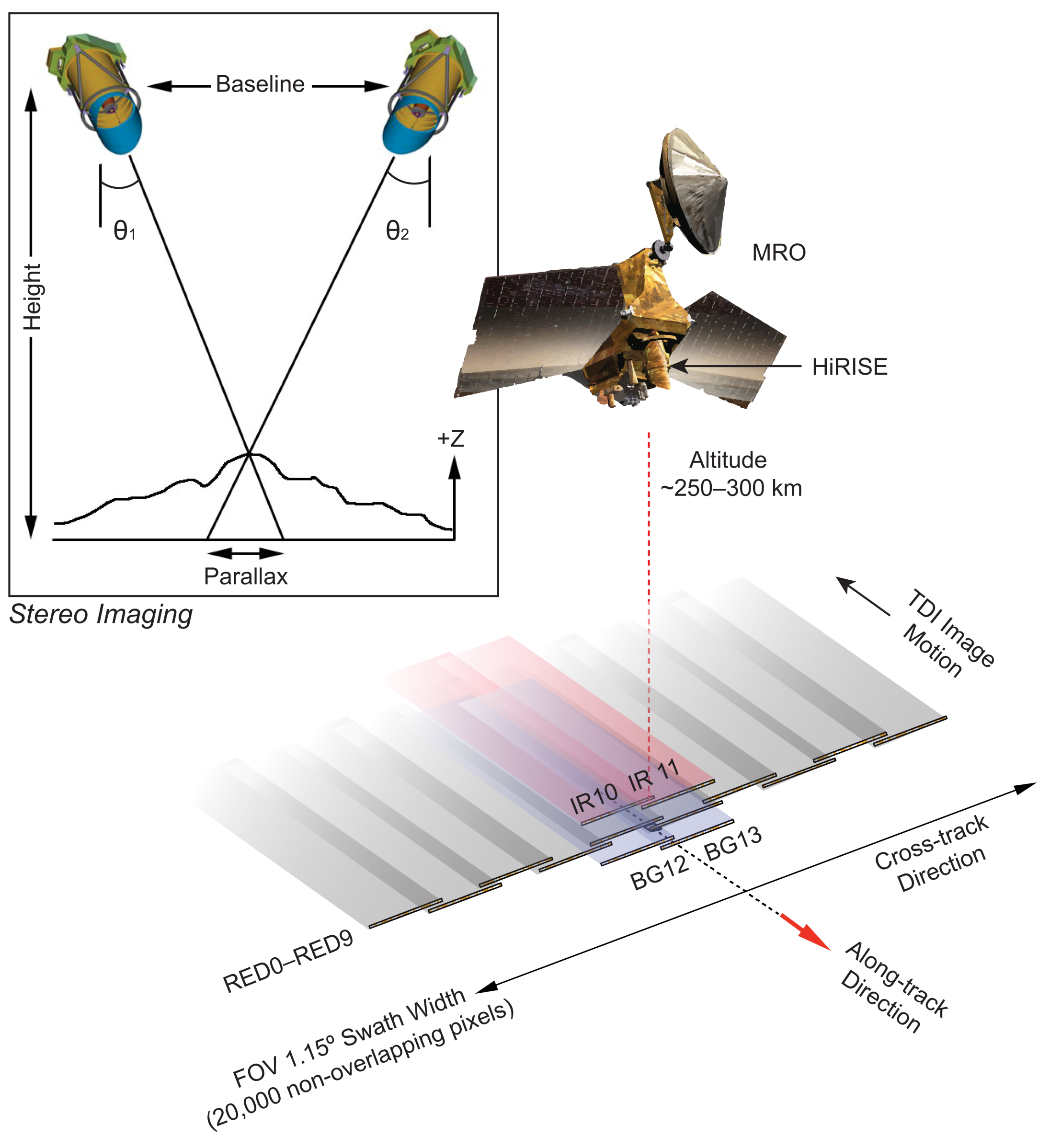
1.1. HiRISE Instrument Characteristics

MRO launched 12 August 2005, and has been in operation at Mars since March 2006 [1]. HiRISE [29] is a nadir-pointing camera with a 0.5 m diameter primary mirror that images in pushbroom mode. The focal plane consists of a staggered array of fourteen charge-coupled devices (CCDs). The active area of each CCD detector is 2048 px wide (in the cross-track direction) by 128 px long (in the along-track direction). This allows for time delay integration (TDI) in the along-track direction, of up to 128 stages, thereby increasing the signal-to-noise ratio (SNR) and dynamic range of HiRISE images [30]. The swath width is spanned by ten detectors offset on the focal plane such that each detector overlaps the adjacent ones in the cross-track direction by ∼48 px (Figure 1). Thus, a HiRISE image can be up to 20,048 px across, and of arbitrary length (with a footprint size of ∼6 km wide by up to ∼120 km long), depending on imaging mode, memory allocation, and thermal constraints. Each CCD has two channels (e.g., RED0_1 and RED0_0) that are read out individually. The ten CCDs, named RED0–RED9, collect visible light in the 550–850 nm range. The central ∼20% of the full swath is covered by four CCDs positioned above and below the RED detectors so that they overlap two RED CCDs in the along-track direction, providing three-color imaging. Two of the central CCDs collect light in the visible blue-green range (400–600 nm), while the other two collect non-visible light in the near-infrared range (800–1000 nm). The four “color” CCDs—named BG12, BG13, IR10, and IR11—provide enhanced information about the surface composition [31]. The staggered layout of the CCDs also allows for the measurement of surface features observed at different times in the overlapping portions of the image strips, which is used for the correction of spacecraft jitter in HiRISE images.

HiRISE has an instantaneous field of view (IFOV) of 1 $\mathsf{\mu }$rad, resulting in a nominal 30 cm pixel scale and a 6 km swath width from MRO’s ∼300 km altitude orbit [29]. One of 14 CCD detector electronics (RED9) on HiRISE failed in 2011; fortunately, RED9 is at the edge of the 10 RED CCDs, so the images became 10% narrower, reducing the footprint width of a typical HiRISE image from 6 km to 5.4 km rather than creating a gap in the middle of the images [32]. Actual pixel scale and image width can vary slightly depending on off-nadir pointing, terrain elevation, and position in the elliptical orbit. Pixel scale also depends on the binning mode used. HiRISE can bin CCD pixels on-chip, for various modes such as bin1 (no binning); bin2, corresponding to ∼60 cm/px; bin4, corresponding to ∼120 cm/px; and other binning modes that are rarely or never used. The most common imaging modes incorporate bin1 and bin2 [33]. Color CCDs (BG and IR) are usually binned to increase SNR to better than 100:1. In the downlink processing pipelines, the image data from binned CCDs are then enlarged by the appropriate factor to match that of the lowest binning mode, typically that used for the RED CCDs. Binning and the number of TDI lines (128, 64, 32, or 8) are two of the parameters adjusted during planning for each HiRISE image to avoid saturation and to optimize SNR, spatial resolution, spatial coverage, and data volume. Some imaging modes include setting the central RED CCDs (RED3/4–RED6) at bin1, while the others (RED0–2, RED7–9, BG11–12, and IR10–11) are set at bin2 or bin4.

As of December 2021, HiRISE has covered 0.4% of the surface of Mars with unique stereo coverage, comprising 6931 stereo pairs. HiRISE has also covered ∼2.6% of the surface uniquely, excluding targeted repeat images for monitoring changes and for stereo targets.

1.2. MRO/HiRISE Stereo Planning

HiRISE is unable to point independently of the spacecraft, so to acquire stereo image pairs, MRO must roll off-nadir by up to 30${}^{°}$ to target the same surface feature on different orbits (Figure 1) [1]. The near-polar orbit means that the nominal revisit time can be up to 17 days, depending on latitude. Other operational constraints such as roll limits, temperature and memory limits, as well as competing science targets, meaning that the second image of a stereo pair is not typically acquired at the first opportunity. Difficulty in achieving the minimum revisit time presents a challenge for acquiring stereo pairs, as the optimal situation is to have as little change as possible in illumination angles and surface features between images. MRO’s orbit is Sun-synchronous, passing over the daylit equatorial region nominally at 15:00 ± 15 min. local mean solar time (LMST). However, the orbit was migrated during 2020 to 15:40 LMST to coordinate with the entry, descent and landing of NASA’s Perseverance rover, returning to ∼15:10 LMST by the end of 2021. Although MRO observes all parts of the daylit surface at approximately the same LMST (except for descending orbits in the polar regions), the subsolar latitude changes by 50${}^{°}$ from summer to winter solstice, so it is inevitable that shadows will move during the period between revisits. There can also be albedo differences due to dust movement or frost changes, as well as changing atmospheric dust or hazes.

The HiRISE operations team developed an internal planning tool—HiRISE Stereo Effect Analysis Software (HiSEAS)—to assess the quality of planned potential stereo pairs based on predicted illumination angles, solar azimuth difference, shadow tip difference, and convergence angle (cf. [34]). MRO observations are planned in two-week cycles; during the course of each cycle, there are often several candidate orbits for a second image of any given stereo pair. HiSEAS identifies which orbits match the illumination conditions of the first image (i.e., incidence angles 30${}^{°}$–60${}^{°}$, and within 10${}^{°}$ of each other) and those orbits that provide an acceptable convergence angle. An acceptable convergence angle is ∼15${}^{°}$–30${}^{°}$, with a larger angle being better for flatter topography, and a smaller angle being more desirable for rougher or steeper topography to minimize potential obscuration of surfaces. Observations can then be planned on both orbits to acquire a stereo pair within one two-week planning cycle, referred to at HiROC as a Stereo Pair Orbits Restricted to a Cycle (SPORC). Stereo pairs acquired as a SPORC or SPORC-like pairs (acquired within two weeks, if not within the same planning cycle) are optimal for DTM production as they have similar illumination angles and minimal expected differences in surface features/albedo, and therefore minimize the need for interactive editing. In practice, acquiring SPORC pairs is challenging, except in polar regions (where the center of the target is poleward of ±65${}^{°}$ latitude and MRO overflights are more frequent). Outside of SPORCs or SPORC-like pairs, the second half of a stereo pair is planned for a later time when the illumination conditions closely match those of the first image. Second half stereo images may be acquired when the subsolar latitude is similar within the same Mars year, or one or more Mars years later. If the illumination angles are within specifications for such delayed second half stereos, this strategy works well in areas where minimal morphologic and albedo changes have occurred.

2. Methods

In this section, we describe the methods used by the HiRISE team to create DTMs with an emphasis on the techniques specific to generating data to be used for change detection. We use the term “digital terrain model” (DTM) rather than “digital surface model” (DSM), and we do not make a distinction in this paper between DTM and “digital elevation model” (DEM). A HiRISE DTM describes elevation in a raster image format, with each pixel assigned a 32-bit signed, floating point value representing elevation in meters relative to the areoid (Martian geoid), to be consistent with the global topography derived from the Mars Orbiter Laser Altimeter (MOLA) [35]. HiRISE DTM pixels represent elevation values at evenly spaced “posts”. The DTM pixel size is also referred to as the ground sample distance (GSD).

In addition to topography, orthorectified images (orthoimages) are the other major data product resulting from DTM production. Orthoimages are projected orthographically onto the DTM. This process removes the perspective of the original viewing geometry, reducing the effects of topography on feature visibility. Orthorectification is crucial for accurate photogrammetry, for measuring surface changes at the pixel level, and for correlation of image and topographic features. Besides orthorectifying the source stereo images, a time series of orthoimages, which were acquired at different viewing geometries and illumination angles, enables precise change detection studies across multiple seasons and years.

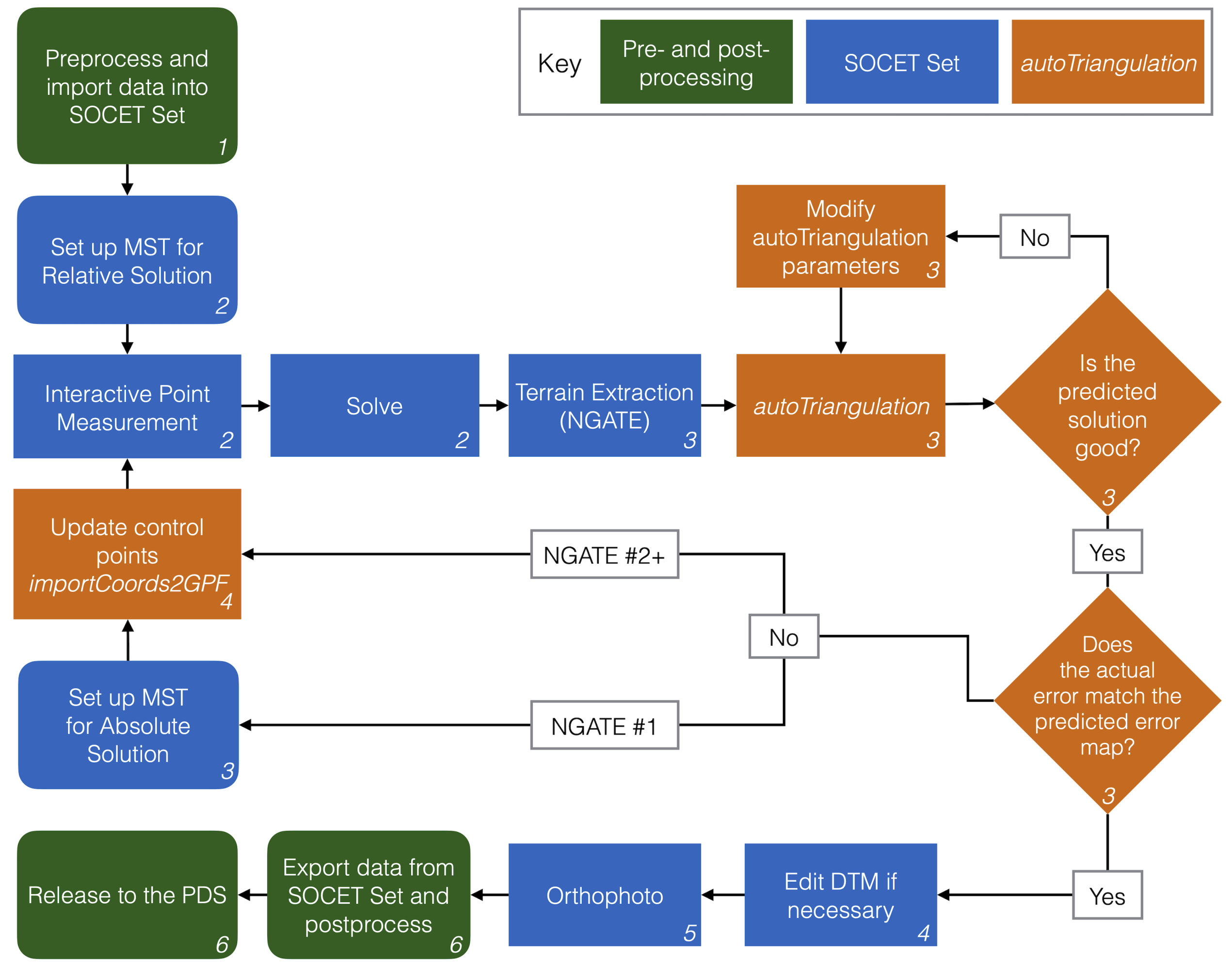
2.1. Creation of DTMs Using ISIS and SOCET Set Workflow

The processing chain starts by preprocessing HiRISE images in ISIS to calibrate and convert them to the formats and generate metadata expected by SOCET Set v5.6.0 [23]. Photogrammetric processing occurs within SOCET Set through a combination of automated and interactive steps. The majority of interactive steps take place during the bundle adjustment stage, referred to in SOCET Set as Multi-Sensor Triangulation (MST). Following MST, the DTM is created in the terrain extraction stage, which is largely automated. The files are then exported from SOCET Set for post-processing in ISIS to convert back to planetary coordinates and map projections in standard formats. The final step is validation of the products and archiving with the PDS. Each of these stages is described briefly below with an emphasis on how the quality of the final product is affected (Figure 2).

2.1.1. Preprocessing

Processing of HiRISE data begins with the engineering data records (EDRs) [36], which contain the raw image data downlinked from MRO. Each EDR is one of two channels that comprise each CCD. The ISIS application hi2isis ingests the raw channel data into the native ISIS image file format, referred to as an image cube. Each channel is then run through hical, which performs radiometric calibration [37]. The radiometric calibration step corrects each detector column for gain, offset, and dark current, and converts the pixel values to units of reflected irradiance over solar flux (I/F). The channels are joined to create one image cube for each CCD using histitch. Additional steps performed by the downlink and image processing pipelines at HiROC reduce noise and balance the brightness across overlapping regions of adjacent CCDs. Radiometric calibration artifacts generally affect an entire channel or CCD. Variations in electronic noise across channels or CCDs can subtly affect the quality of the DTM.

After radiometric calibration, precision geometric calibration is performed to remove distortion across the focal plane due to the optical curvature of the beam, remove the CCD offsets, and optionally correct for spacecraft jitter. All three of these corrections are accomplished by the HiPrecision subsystem at HiROC [38]. HiPrecision has two processing branches: one to correct for the nominal optical distortion and CCD offsets (HiNoproj), and the other, HiRISE Jitter-Analyzed CK (HiJACK), to apply an additional correction to images that have increased spacecraft jitter.

HiRISE is subject to image distortions by high-frequency jitter due to its pushbroom mode of image acquisition and is more sensitive to the effect than other cameras because of its small IFOV. Although jitter distortions in individual HiRISE bands are typically invisible to the naked eye, they cause misregistration of the BG and IR bands to the RED overlapping CCD images resulting in obvious color fringing. Similarly, jitter distortions cause poor stereo image correlation. In the color processing pipelines at HiROC, the IR and BG bands are transformed to match the RED band, producing accurately registered 3-band color images. However, this relative correction does not remove the jitter from the RED data, which are the source images in HiRISE DTM production. The combined effects of jitter in one or both images in a stereo pair can cause artifacts in DTMs where the stereo correlation algorithm fails or where the elevation values are misestimated. Such artifacts are discussed in more detail in Section 2.3.2. Efforts are made to mitigate jitter in HiRISE images as much as possible by enforcing high-stability mode on MRO (pause motions of the solar arrays and Mars Climate Sounder [39]) during stereo image acquisition, and by performing image correction on the ground when necessary. Images with >0.5 px mean jitter magnitude are typically improved after jitter correction; however, not all jitter frequencies may be removed (Figure 3).

The ISIS program noproj projects each CCD image strip into an idealized camera model space. The “ideal” HiRISE camera model is a 20,000 px wide single-detector pushbroom camera, with the boresight at the center of the image, and CCD offsets removed [23]. The noproj-corrected images for each CCD are then mosaicked to produce a full-swath width, non-map projected image in the RED band. The pixel values within the noproj mosaic are converted from 16-bit to 8-bit digital number (DN) values and exported from ISIS cubes to a raw image format. The pushbroom sensor model plugin developed by the USGS for SOCET Set is a rigorous physical model based on geometric optics. The camera position and attitude are modeled as continuous functions of time by being broken into a fixed part that is interpolated through an arbitrary number of values supplied when the image is imported, and an adjustable part that is represented by a low-order polynomial (order 2 for position, 3 for Euler angles). The generic model includes the possibility of radial optical distortion, but the pre-processing in ISIS corrects such distortions in the images, so this capability in SOCET is not used.

For image import with initial position and pointing information, SOCET Set requires the image metadata in a text file format which is generated by socetlinescankeywords (i.e., “SOCET linescan keywords”). The keywords required by SOCET Set include the camera parameters, image information, and information about the spacecraft trajectory and pointing obtained from the Spacecraft Planet Instrument C-matrix Events (SPICE) kernels [40].

Additional data are prepared for the project setup in SOCET Set, such as global reference topography, geographic coordinates, and approximate elevation values. Laser altimetry from MOLA is obtained over a region centered on the HiRISE stereo pair and padded by 0.5${}^{°}$ in latitude and longitude. Crossover-corrected MOLA Precision Experiment Data Records (PEDRs) [35] are the primary dataset used to provide absolute spatial control. The MOLA global DTM, or Mission Experiment Gridded Data Record (MEGDR), which is interpolated from the crossover-corrected global PEDR data, is also extracted and clipped to the same region and exported as an ASCII (plain text) format file. All of the preprocessing occurs in the Unix environment. The raw images, keywords files, MOLA PEDR and MEGDR files, and the project location information are then transferred to a workstation running the Windows operating system for import and processing in SOCET Set.

2.1.2. Bundle Adjustment

Bundle adjustment, which is performed with the Multi-Sensor Triangulation (MST) tool in SOCET Set, is the process of controlling the images to each other and to a reference elevation dataset. The inputs are image-to-image feature correspondences (“tie points”) and usually image-to-ground correspondences (“control points”). SOCET Set provides tools for measuring these inputs interactively via Interactive Point Measurement (IPM) and by automated matching (Automatic Point Measurement, APM). The outputs are revised estimates of camera position and pointing parameters that minimize mismatches at the points in a least-squares sense, as well as the ground coordinates of the tie points. The quality of the solution largely determines the absolute accuracy of the DTM, and influences how well the stereo matcher can extract elevation values from the stereo images, which affects internal precision. We set image control precedence (i.e., “left eye” and “right eye” which can be set arbitrarily in IPM) by selecting the image with the lower emission angle (nadir-most) to be the control, as it should have the least amount of distortion or obscuration due to topography. MST weighting of exterior orientation parameters serve to: (a) weight position adjustments at roughly the level of uncertainty associated with the reconstructed trajectory [41,42]; (b) weight angular adjustments to allow changes in the ground coordinates of pixels comparable to those resulting from the allowed position adjustments, or the uncertainty in attitude reconstruction (if that is known), whichever is larger; and (c) weight the higher order (velocity and acceleration) parameters so that they allow variations of the same magnitude over the period of time elapsed in acquiring the image. The uncertainty requirements for MRO in the reconstructed spacecraft position and camera pointing are 100 m along-track, 40 m cross-track, and 1.5 m radially [43].

A relative adjustment is performed first to tie the stereo images together, which removes any along-track offset resulting from camera pointing uncertainty. A minimum of 16 evenly distributed tie points are created with either IPM or APM. The solution is considered acceptable if the root mean square (RMS) error is <0.7 px, and is typically <0.5 px, but because of the prevalence of along-track jitter, the residuals in the line (along-track) direction are often higher than desired. Residuals in the sample (cross-track) direction are expected to be <0.1 px. The implementation of jitter correction and SPORC targeting has resulted in RMS values typically in the 0.1–0.3 px range for an HiRISE stereo pair.

Preliminary elevation control is provided for one or two of the tie points to bring the model into approximate agreement with the MOLA topography. After solving, if the RMS and line and sample errors are deemed acceptable, the solution is saved. The effect of saving a solution is to update the position and orientation parameters in the support files for the images, resulting in an improved stereo model. The improved model can be seen in the viewer when the images are reloaded. At this stage, no image resampling has yet been performed; the model exists in the mathematical sense, not as a digital terrain file.

2.1.3. Terrain Extraction

Once a relative solution with an acceptably low RMS (<0.7 px) is achieved, including preliminary elevation control, an initial terrain model is generated. The goal of generating this initial model is to measure the quality of the fit to MOLA and to evaluate the preliminary topography, not necessarily to produce the final DTM. The algorithm used by SOCET Set for terrain extraction is called Next Generation Automatic Terrain Extraction (NGATE) [44]. An optional step after running NGATE is to run the Adaptive Automatic Terrain Extraction (AATE) [45] algorithm with a one-pass strategy. Using AATE essentially provides a moderate smoothing of the characteristically blocky texture of the NGATE product, which improves the accuracy of slope estimates over short baselines while having little impact on the elevation values [46,47]. Running AATE is considered an optional step because in some cases it can worsen interpolation artifacts (e.g., [23]), and can also introduce tiling lines. Simply smoothing the output of NGATE with a lowpass filter is a viable, and faster alternative to smoothing with AATE [47].

After NGATE finishes successfully, the terrain quality is examined for major blunders or artifacts. This qualitative check is most easily accomplished by opening the file in the Interactive Terrain Edit (ITE) application and rendering it as a shaded relief image. Terrain files can be visualized in ITE either as vector graphics (e.g., as contours or dots), or as a raster file in the form of a shaded relief image. The shaded relief image is generated as a grayscale image to provide information at a glance about the surface texture of the terrain model. Artifacts or failures of the stereo correlation are readily visible in the shaded relief image, especially if the illumination direction is set in such a way as to accentuate artifacts such as CCD seams. Once identified, some artifacts can be edited if they are relatively small, and in areas of scientific interest (Section 2.1.4). Many artifacts (such as those due to jitter) are systematic, occurring throughout the DTM (Figure 4a,b,f,g). Error in the line direction interferes with image matching and thus causes noisy terrain, or larger artifacts such as the “boxes” of noisy interpolation (Figure 4a,b). These can sometimes be improved by manually measuring additional tie points in those areas. Error in the sample direction causes misestimation of elevation. Periodically varying error in the sample direction is a signature of uncorrected spacecraft jitter, which produces ripples in the DTM, parallel to the cross-track direction (Figure 4f). Faceted textures result from interpolation over bland, shadowed, or low-contrast areas in the images (Figure 4c). The stereo correlator often fails over dark dunes with ripples (Figure 4d). Areas of failed stereo correlation are interpolated over deeply shadowed terrain, or areas where surfaces are obscured in one of the stereo images due to the observation geometry (Figure 4e). If it is unclear whether a feature is real or an artifact, the DTM should be validated by comparing it to the source stereo images.

The preliminary model is used to assess the fit to MOLA, with the goal of obtaining a transformation that minimizes differences between the HiRISE DTM and the MOLA PEDR elevation values. Within SOCET Set, the quality of the fit to MOLA can be assessed by eye in the image viewer, but a coarse sampling of the elevation differences may not reveal patterns of misfit in the registration. The built-in SOCET Set command line tool, dtm_compare, generates a difference map between two DTMs. In the HiRISE case we use dtm_compare to measure the elevation differences between HiRISE and the MOLA gridded data (or between two HiRISE DTMs, Section 2.2.1), which as noted may contain interpolation artifacts, or miss features entirely that are present in the images. For polar DTMs, dtm_compare is useful as the high orbit-track density of MOLA at higher latitudes reduces interpolation errors in the gridded data. However the gridded data contain some noise due to the variability in MOLA orbits over many seasons and Mars years [48].

Although the SOCET Set allows for manual adjustment of geographic control points in IPM, the goal is to remove subjectivity from this process as much as possible and to fit the HiRISE stereo pair to the MOLA data in a rigorous and objective (as well as automated and efficient) way. One method is to use the pc_align routine, which is distributed with Ames Stereo Pipeline (Appendix B). The pc_align tool uses an Iterative Closest Point (ICP) algorithm to match a dense point cloud to a sparse point cloud, which is appropriate to the HiRISE-to-MOLA models. The resulting transform can be used to update the position of the images in SOCET Set. As an alternative to using ASP, the HiROC team developed a Windows command line tool called autoTriangulation [49], which is freely available (

Table A1. List of programs referred to in the text, with URLs if available.

Software/Application	URL (If Applicable)
Ames Stereo Pipeline	https://doi.org/10.5281/zenodo.598174, accessed on 10 March 2022
pc_align	stereopipeline.readthedocs.io/en/latest/tools/pc_align.html, accessed on 10 March 2022
ISIS	https://doi.org/10.5281/zenodo.2563341, accessed on 10 March 2022
hi2isis
hical
histitch
noproj
socetlinescankeywords
SOCET Set v.5.6.0
dtm_compare	(SOCET Set internal command line program)
HiROC
HiSEAS	(code maintained internally by HiROC)
autoTriangulation	https://www.uahirise.org/tools/at/, accessed on 10 March 2022

). The autoTriangulation tool is used by the HiROC team on all non-polar DTMs, providing there is at least some MOLA PEDR coverage. In the rare cases where there are no MOLA PEDR data within the HiRISE stereo coverage, CTX stereo images may serve as an intermediate resolution control. This situation is more likely to occur at lower latitudes, where MOLA tracks are more widely spaced due to the near-polar orbit of MGS. If CTX stereo is not available, a best effort fit to the MEGDR (gridded) topography may be sufficient, although there may be large interpolation artifacts in the MOLA data. In this situation, autoTriangulation is not applicable.

The inputs required for autoTriangulation are the terrain model from NGATE exported as a GeoTIFF (raster format with geospatial information), the MST solution report file, and the 3D altimetry point file. AutoTriangulation measures the initial fit to MOLA (difference of the elevation values for each MOLA PEDR, averaged over the MOLA footprint, and the elevation of the corresponding location in the DTM), and then iterates through a series of translations and rotations to minimize the elevation differences, subject to statistical filtering that is weighted based on thresholds for the mean and standard deviation of the errors for each MOLA orbit. The outputs of autoTriangulation are a map of the initial fit and the predicted solution (Figure 5), a map of the input ground points and their translated locations, a map of the weightings assigned to each MOLA orbit, and a text file report of the translated ground point coordinates. The polar DTMs exported as a GeoTIFF from SOCET Set do not contain the correct map information and therefore cannot be compared to the MOLA data in the version of autoTriangulation currently available. Polar DTMs are controlled manually to MOLA data, or are produced as models with relative elevation values.

An acceptable predicted solution from autoTriangulation has a mean elevation difference near zero, and a standard deviation of less than 5 m. To apply the predicted coordinate transformation, another program bundled with autoTriangulation (importCoords2GPF.py) updates the coordinates of all the tie points within SOCET Set. Although the points are all moved in the X, Y, and Z directions, it is not practical, nor necessary, to set all of the existing tie points to be XYZ-control points in IPM. The operator chooses one or two points to convert to XYZ-control (one point translates, two points translate and rotate the model), and converts an even distribution of the remaining tie points to Z-control. The weighting accuracies for the control points are set to 5 m, as the solution is self-consistent, and the expected accuracy is within 5 m. An additional required step to apply this “absolute” solution is to allow both images to now adjust. The original support files for the stereo images are reloaded (prior to any solution), and the Solve step is performed. Solving is performed on the original (unadjusted) support files to ensure that the solution is applied to the original position state. The solution results will include X, Y, and Z errors in units of meters, in addition to the RMS error, if there are two or more XYZ-control points.

We expect the errors controlling HiRISE to MOLA to be within 100 m in the X and Y directions and to be within 5 m in the Z direction, based on the differences in spatial resolution between MOLA and HiRISE. These values are consistent with an analysis of overlapping HiRISE DTMs controlled individually for landing site assessment, which found the absolute positional accuracies to be 50–100 m in X and Y and 10–20 m in the Z direction [50]. In practice, the errors are typically much lower than that, on the order of a few meters. The error in X, Y, and Z reported after applying a solution from autoTriangulation is typically low, as the translation is rigid and applied across all points. The images are reloaded to apply the updated solution, and the fit to MOLA PEDRs is assessed visually in the Image Viewer.

If the updated solution actualized in SOCET Set corresponds to the predicted solution from autoTriangulation, then a second NGATE run is performed (Figure 2). Generally, the initial relative solution should be close enough to the correct location that autoTriangulation optimizes the transformation in one step, and the solution within SOCET Set achieves the same result. However, since autoTriangulation applies a rigid translation and/or rotation of the DTM and is not constrained by fitting to the parameters in MST, the implementation of the transformation may not be in agreement after solving in SOCET Set. In that case, the process of adjustment is repeated by either manually placing or adjusting Z- or XYZ-control points, or by using autoTriangulation to predict and implement a new solution, until a satisfactory fit to MOLA is achieved. In the best case, this process takes two iterations, but in practice it may take multiple attempts through MST to get an acceptable result. In any case, the absolute control solution is considered to be successful when the actual difference and the predicted difference reported by autoTriangulation are similar and within the expected accuracy range (e.g., Figure 5b). A solution with a low RMS value and a good fit to MOLA will result in better DTM quality, as the model is more physically realistic. At this point, the triangulation step is complete. The NGATE result is then evaluated to determine if editing is necessary. The shaded relief image is the easiest way to identify at a glance areas that might require editing.

2.1.4. Editing

The capability to perform interactive editing on the DTM is one of the advantages of using SOCET Set, but it is also time consuming, and requires a high degree of skill by the operator. It also can introduce a degree of interpretation by the human operator that may or may not be acceptable depending on the artifacts, their location, and the intended use of the DTM. It is therefore desirable to keep editing to a minimum, and to clearly denote for the end user the locations of any manual editing. Some artifacts (particularly spikes or pits due to shadow edge differences between stereo images) in the DTM can cause distortions in the orthoimages, particularly in off-nadir images, which negates the ability to measure changes in surface features. Edits to improve the model in and around areas of scientific interest are carried out cautiously, and only if the surface can be reliably identified in both images by the operator. A common situation that requires editing is over dark dunes, where the stereo correlator often fails due to the surface being smooth and low contrast. Precise measurements of changes in aeolian bedforms is an area of active research with HiRISE images, and so editing of terrain over dunes is often necessary.

SOCET Set’s Interactive Terrain Editing (ITE) tools include a geomorphic editor (interpolates across lines and curves), various area editing algorithms, and a post editor. The geomorphic tool is useful in specific situations such as along the interior of crater walls, where a line can be drawn along a path of relatively constant slope. The most commonly used tools for HiRISE are the area editor algorithms “first order interpolation” and the Triangulated Irregular Network (TIN) editor. The TIN editor tool extracts the posts within a polygon specified by the operator, converting them from gridded posts to a TIN, which can then be edited by manipulating the vertices of the triangles. The TIN editor is used extensively in editing terrain over dunes. After edits are complete, the TIN within the boundary is transformed back into gridded posts. First order interpolation is used to smooth areas within a polygon drawn by the operator and is most useful removing small spikes or pits. It can also be effective in deeply shadowed areas, but the larger the polygon, the more likely additional cosmetic effects will be introduced that may or may not be acceptable. The post editor is the least used, as a typical HiRISE DTM contains millions of posts, and editing them one at a time is inefficient, even over a small area. Edited areas in HiRISE DTMs should be noted and analyzed with caution. The edits are typically carried out manually, and therefore introduce some level of subjectivity into the representation of the topography.

Every post in the gridded DTM is assigned a Figure of Merit (FOM) value encoding the correlation quality, whether a post has been manually edited, or whether it has been automatically interpolated or otherwise failed. SOCET Set FOM values range from 1–99 and are mapped into eight classes (

Table A2. FOM values output from SOCET Set, with the corresponding classified map color and description.

SOCET Set Values	FOM Map Color	Category Description
1	Black	No data, outside boundary
2	Dark blue	Shadow (if designated as such)
3, 5–20, 28, 31–39	Orange	Suspicious (edge, corner, did not correlate,
		other bad value, derived from seed DTM)
4, 30	Red	Interpolated/extrapolated
		(e.g., from neighbor pixels)
21	Pink	Saturated (in source images)
22–27, 29	Cyan	Manually edited/interpolated or smoothed
40–59	Yellow	Low end of good correlation range
60–99	Sea Green	Good correlation

). The classification scheme is based on a balance between what information could be the most useful to the user, and how the quality information is encoded in SOCET Set. HiRISE FOM maps are generated at the full scale of the corresponding DTM and display classified FOM values draped over a shaded relief image. The FOM maps are created in the JPEG2000 format at full scale and are released as PDS “Extras”, which are ancillary files intended to assist in browsing or visualizing the standard data products [51]. The full-scale product allows the end user to determine the suitability of any area of the DTM for analysis by being able to overlay the FOM with the images and the DTM. Areas designated Manually Edited/Interpolated should be evaluated compared to the images and the DTM to determine if the edits accurately reflect the topography. Low Correlation and Suspicious areas are typically due to low contrast, bland, or noisy areas in the images. They should also be evaluated before performing any analysis to judge how well the stereo correlator captured the topography. Deep shadows in the stereo images result in no reliable elevation data and are designated as Shadowed in the FOM map. Such areas are rare in HiRISE DTMs, but an example of one DTM with a large, shadowed area is shown in Figure 6. Data gaps in one or both of the stereo images are indicated as No Data. Areas of Good Correlation are reliable and accurately reflect the topography, within the error limits of the DTM.

2.1.5. Orthorectification

Orthorectification is a projection of images onto a DTM, which effectively removes the perspective due to the original observation geometry. The image pixels undergo a transformation and interpolation to place the viewpoint in the vertical direction (and from infinite distance) over every pixel of the terrain model. Prior to this step, the images have not undergone any transformations within SOCET Set. The boundary of the DTM defines the boundary of the orthorectified stereo pair. We use the DTM boundary to define the extent of additional (non-stereo) images orthorectified to the stereo model, regardless of their actual coverage. This may result in null pixels where the DTM exists, but there is no image coverage. In practice, the consistent image dimensions and data extents facilitate time-series analysis.

HiRISE orthoimages are typically produced at two scales: one that matches the scale of the DTM, and one at the native map projected pixel scale of the source image. For example, if the DTM has a GSD of 1 m, and the source image is 25 cm, then two versions of the orthoimage are produced: one at 1 m/px, and one at 25 cm/px. The two versions of each orthoimage are produced for the convenience of the end user. It is beneficial to have the highest resolution orthoimages when performing change detection analysis or detailed mapping. The higher resolution version of the orthoimage is also intended to be comparable to the corresponding reduced data record (RDR). However, the orthoimages undergo at least two resamplings, and therefore may appear slightly smoother than the corresponding RDR. The smaller file size of the lower resolution orthoimage is a convenience for use in geospatial applications along with the corresponding DTM.

The color (BG and IR) images are not used in the terrain generation, but when possible, these images are orthorectified to create 3-band (IR, RED, and BG) orthoimages, also in two resolutions. The color strips are preprocessed through the radiometric calibration and CCD stitching and balancing steps in the HiROC processing pipelines. Jitter correction for the color data is performed in a relative sense, where the color images are shifted row by row to match the jitter distortions measured between the BG/IR and corresponding RED CCDs. Each band is imported into SOCET Set, and in the same step the updated solution parameters achieved in MST using the full RED swath are applied automatically. Each band is orthorectified individually and then exported and stacked in post-processing to produce a 3-band color image, similar to the IRB HiRISE Color RDR product [31,36].

2.1.6. Post-Processing and Data Archiving

The DTM and orthoimages are exported from SOCET Set using the programs dem2isis3 and ortho2isis3, both developed by the USGS and built against the SOCET Set binary. These export routines convert the files from the internal SOCET Set rasters to a RAW image format and generate an associated shell script to be run on the Unix processing cluster. The shell script contains the ISIS commands that will reproject from the map definition native to SOCET Set to the ISIS cube format with planetary mapping definitions. The DTM and its FOM map are exported together with one shell script that converts both files. Each orthoimage is exported with a corresponding shell script file.

The ISIS cubes are resampled once to remap them to square pixels at the project center latitude. SOCET Set accommodates pixels that may have different sample and line resolutions, but ISIS (v3+) can only accommodate square pixels. This requires a slight reduction factor during the transformation, which results in the actual GSD of the DTM being some value near to, but not exactly, 1 or 2 m, for the equirectangular map projection. The same reduction factor is used for the orthoimages, which provides a consistent resolution for all files in the project. The DTM and orthoimages are projected onto a spherical shape model of Mars, with a radius defined as the radius of the Mars ellipsoid at the center latitude of the DTM [36].

The ISIS cubes are then converted to standard PDS version 3 (PDS3) formats. The DTM is converted to a 32-bit floating point uncompressed raster with an embedded label (.IMG file extension). Pixel values correspond to elevation in m (i.e., 1 DN = 1 m). The orthoimages are archived as 8-bit losslessly compressed JPEG2000 (.JP2 file extension) with embedded GeoTIFF tagging, and detached labels (.LBL text files). The PDS3 formats, map definitions, keywords, and labels are as similar as possible to those used for the HiRISE RDRs [36].

Ancillary files are produced to enable quick visualization of the data, described as “Extras” or browse images (Figure 7). Each version is provided as a reduced, lossy-compressed (.jpg) image with annotations for the product ID, image credit, and scale bar, and non-annotated browse and thumbnail images. DTMs are not inherently images, and therefore must be displayed in different ways to visualize the elevation data. The “Extras” products for an HiRISE DTM and associated orthoimages include reduced size JPEG format images of the DTM as a grayscale image, as a shaded relief image, and as shaded relief with colorized altimetry. The FOM map is considered an Extra product, but is produced as a JP2 at full scale, with the FOM classes color-coded and overlaid on the shaded relief image. Browse images are produced for the lower resolution version of the orthoimages. A README text file accompanies each project, describing the source data, GSD, producer, quality metrics, notes, FOM value classification, and naming convention.

The HiRISE team releases data to the PDS on a monthly cadence. DTMs and orthoimages produced for the HiRISE team are released the month following their completion. HiROC also archives DTMs produced at other institutions with the PDS, as long as they follow the ISIS/SOCET Set workflow. Deviations from the workflow, such as not controlling the model to MOLA, can be accommodated, and are noted in the accompanying README text file. Approximately two thirds of the HiRISE DTMs currently available in the PDS were produced at HiROC, with one third produced by seven other institutions. As of December 2021, 834 DTMs and 2732 unique orthoimages have been released to the PDS and are available to the public via the PDS and at (https://www.uahirise.org/dtm/, accessed on 10 March 2022) (Figure 8). The HiRISE catalog is available in PDS3 format. Plans to deliver PDS4 compatible products alongside the existing PDS3 products are currently in development.

2.2. Tying in Additional Images and DTM Mosaicking

Change detection studies are facilitated by orthorectifying multiple images acquired at different times over a target where a DTM exists. The additional images need not be constrained to the lighting and geometric requirements of a stereo observation. Indeed, variable illumination and observation geometry may be unavoidable to monitor seasonal processes. The preprocessing approach is the same (Section 2.1.1), except there is no need to analyze MOLA data. Jitter correction is not as widely applied to additional (non-stereo) images, as they will not be used for terrain extraction, and we want to minimize the number of times the image pixels are transformed and interpolated. Jitter correction does transform the images; therefore, it is not applied unless the jitter is of a large enough amplitude (>1 px) that might negatively affect change detection studies. At this time, color orthoimages are not produced for jitter-corrected images on a regular basis.

Additional images and their corresponding keywords files are imported into a new or existing project in SOCET Set in the same way as the stereo pair. The extra images may be controlled at the same time as the stereo pair, or they may be added later. It is more straightforward to control the stereo pair first, separately, in order to achieve the best solution and generate the DTM. The addition of multiple images does not change the original stereo solution. The procedure for tying in the additional images is performed manually. The RMS error from a solution in MST that includes multiple images may be higher than for a single stereo pair, but it is more important to achieve the best visual results rather than the smallest RMS value. To achieve the desired total RMS error of <0.7 px, any points with high (>1.0 px) line or sample errors are identified and remeasured manually until their errors are brought down sufficiently.

After solving and reloading the images, the quality of the fit is assessed in the stereo monitor by checking the vertical offset between the stereo pair and the additional images. The stereo pair used to generate the DTM is held fixed during this process. Each additional image is allowed to adjust until the vertical offsets between it and the stereo pair are <1 m. Horizontally shifted pixels result from vertical offsets, because differences in the stereo viewer equate to differing parallax between the image pairs. Special emphasis is placed on achieving as good a fit as possible in areas of scientific interest. In these areas, additional tie points may be added to improve the fit. After MST is completed for all additional images, they are orthorectified to the DTM generated from the stereo pair used for control.

2.2.1. Multiple DTMs for Volumetric Change Detection

The goal of generating multiple DTMs over a given target is to measure topographic changes (i.e., volumetric changes). The procedures for controlling multiple stereo pairs to create multi-temporal DTMs of the same target is essentially the same as that for tying in additional images for orthorectification. It can be preferable to control stereo pairs for multi-temporal DTM generation simultaneously [52], using stereo pairs acquired at similar seasons for similar illumination. This allows all the images to adjust together to achieve the optimal solution. However, in many cases, the DTM already exists, and new stereo images are tied to the existing model, holding the original stereo pair fixed. The new stereo pair is treated as any other set of additional images in all steps, except jitter correction may be applied for the sake of improving terrain quality. In the situation where a DTM already exists, the MST setup is performed by holding the original stereo pair fixed and allowing both images in the new stereo pair to adjust relative to the original pair. The locations of existing tie points and control points are measured on the new images. Thus, in the case where one or more new stereo pairs are being tied to an existing model, the original HiRISE DTM is used as the elevation reference rather than MOLA data, with elevation reference points used in non-changing areas.

Before running NGATE with the new stereo pair, the solution is validated by measuring the elevation differences between the two models, particularly in the parts of the scene that contain non-changing surfaces. Differences are spot checked, with particular emphasis in areas that will be the focus of analysis. The process of adjusting tie and control points, solving, and checking differences is iterated until the difference between the two models is on the order of 1 m or better for a 1 m GSD DTM (likewise ≤2 m for a 2 m GSD DTM). It is not always possible to find abundant locations with non-changing surfaces throughout the scene (e.g., within dune fields or on steep slopes), so extra care is taken to reduce systematic errors, such as tilt, and to minimize elevation differences in areas of specific scientific interest. After a successful solution is reached, a new terrain model is generated in NGATE. The SOCET Set built-in command line tool dtm_compare is used to generate a difference map between the two HiRISE DTMs.

2.2.2. Mosaicking of Stereo Pairs for Regional Topography

The extent of HiRISE DTMs and orthoimage coverage can be increased by acquiring overlapping and adjacent stereo pairs that can be controlled together in one project to create a mosaicked DTM. Each stereo pair is controlled relatively with an even distribution of tie points (Figure 9a). Additional tie points are added in overlapping areas to tie overlapping stereo pairs to each other. During this process, one image in one of the stereo pairs is held fixed for the relative solution. New tie points are created along seams between overlapping pairs. Once all pairs are controlled in a relative sense, all images are allowed to adjust in the absolute sense, with the addition of XYZ-control points. Tie points in overlapping areas (4-way tie points) are remeasured until the seam has <1 m elevation difference for bin1 pairs, and <2 m for bin2. Each stereo pair is run through NGATE individually, and then merged using SOCET Set’s Terrain Extraction Merge tool. Seams are again checked visually in the merged shaded relief image. The merged DTM is exported for assessment in autoTriangulation so that a best fit to MOLA can be assessed for the whole mosaic (Figure 9b).

In some cases, newly acquired stereo pairs are added to an existing project. In these situations, the existing stereo pair is held fixed, and adjacent pairs are tied in, adding Z-control in the new pairs where necessary using MOLA data. Orthoimages are generated for each stereo pair using their respective DTMs. Each stereo model is exported separately and post-processed individually for release as standard products to the PDS.

2.3. Quality Metrics and Sources of Error

An understanding of the quality of a DTM in terms of its vertical precision and horizontal resolution (e.g., [47]) is necessary to constrain the error in any quantitative analysis. Absolute positional accuracy is also important for some applications though not for others. These quality metrics are especially important for understanding the limits of what can be resolved in sequences of orthorectified images for time series analysis, or for measuring volumetric changes in multi-temporal DTMs over the same target. Many factors affect the quality of a stereo DTM. These include the viewing geometry, imaging modes, time elapsed between stereo images, season of acquisition, dynamic range, atmospheric conditions, image noise or SNR, spacecraft jitter, and the availability and quality of geodetic control. Some of these factors can be measured directly, while others are estimated, or assessed qualitatively.

2.3.1. Precision, Accuracy and Resolution

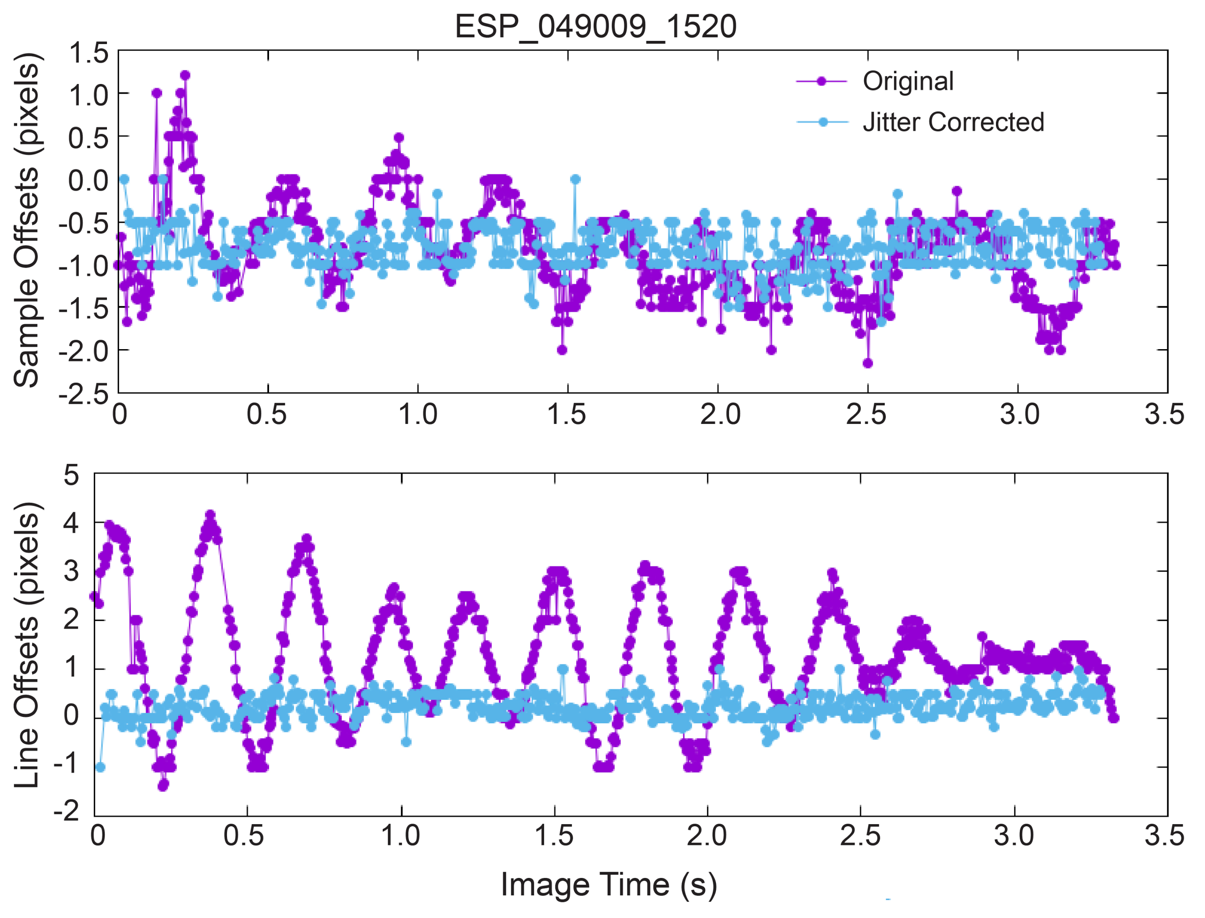
Quality is measured in both the relative and absolute sense, that is, in terms of precision and accuracy. Vertical precision describes how well distances, elevations, and slopes within the DTM can be measured in a relative sense, while accuracy reflects how well the model is controlled to the global topography in an absolute sense. In addition, the user needs to know the effective horizontal resolution of the DTM, to be able to assess the minimum size feature that can be confidently resolved, both horizontally and vertically. Localized errors or blunders viewable in the FOM map are also important to identify to inform the end user what areas within the DTM should be avoided or used with caution.

Vertical precision can be thought of as the relative error (or standard deviation) of the individual elevation values within a DTM. Vertical precision can be predicted based on observation geometry if the reliability of image matching is known, or it can be assessed statistically by comparing the DTM to a known (high) precision reference [47]. Estimated vertical precision (EP) is related to the observation geometry and the pixel scale of the stereo images as well as the precision of image matching ($\rho$) as follows [53].

$$EP=\rho \times GS{D}_{image}/(parallax/height).$$

(1)

The rule of thumb that the matching error ($\rho$) is ∼0.2 px has a long history extending back at least to [54]. A range of studies in which vertical errors were quantified by other approaches and Equation (1) was used to calculate $\rho$ yielded estimates in the range of 0.2–0.3 px (e.g., [23,53]. The actual RMS error reported by MST in SOCET Set (typically <0.5 px) provides another estimate of $\rho$. $GS{D}_{image}$ is the pixel scale on the ground in meters. $Parallax$ is the baseline distance between the camera positions, and height is the average height of the spacecraft above the ground. The $parallax/height$ value can be calculated with knowledge of the spacecraft position at each observation [34]. If both emission angles are relatively small (tens of degrees), $parallax/height$ can be approximated by taking the tangent of the convergence angle between the stereo observations. A further simplification, applicable to HiRISE, is obtained when the stereo look directions lie in the same vertical plane. The sum of the tangents of the emission angles equals $parallax/height$ to a close approximation when (as for most HiRISE pairs) the two images in the stereo pair were taken from opposite sides of the target (Figure 1). If both images are taken from the same side of the target, the difference of the emission angles is used instead. The direction of off-nadir roll can be inferred from the incidence, emission, and phase angles, which are available in the HiRISE RDR labels. If the phase angle is greater than the incidence angle, then MRO rolled to the west, otherwise it rolled to the east (although this relationship breaks down at high latitudes). The use of the tangent of the stereo convergence angle, or emission angles, to approximate $parallax/height$ does not hold at latitudes poleward of ±80${}^{°}$ due to the orbits crossing at oblique angles; in these cases, the full three-dimensional formula [34,55] must be used. For HiRISE DTMs, the estimated vertical precision (EP) is typically better than the GSD, and is on the order of a few tens of cm for a 1 m DTM, or ∼1 m for a 2 m DTM.

The GSD of the DTM, which can be chosen freely as a processing parameter, sets a hard lower bound on the horizontal resolution of the DTM. It is therefore important to choose a GSD small enough to oversample the true resolution of the DTM that results from the image properties and details of the matching process. As long as this is performed, the choice of DTM GSD has a minimal effect on DTM quality, and a convenient (consistent across multiple DTMs and “round”) value can be selected. A longstanding rule of thumb is that the DTM GSD should be roughly three to five times the image GSD. Because DTMs are produced by matching local patterns of pixels between images, and these patterns cannot be much smaller than three pixels across, the true resolution is unlikely to be smaller than this. Ref. [47] recently showed that the horizontal resolution of many Mars DTMs (including examples made with SOCET Set) is in fact larger, typically 10 to 20 image pixels, so the 3–5 px rule could be considered optimistic. The HiRISE team follows the convention of setting the DTM GSD at 1 m for bin1 images (which is ∼3 times the nominal pixel scale of 0.30 m for bin1 images, or 4 times the mapped pixel scale of 0.25 m) and 2 m for bin2 images [29]. HiRISE stereo pairs are sometimes acquired in mixed bin modes. Mixed bin modes may occur within a single image, such as when the RED CCDs in the center of the swath are set to bin1 and the outer CCDs are set to bin2, or within a stereo pair, when one half of the stereo pair is a bin1 image, and the other is a bin2 image. For mixed bin mode stereo pairs, the choice is typically made in favor of the coarser resolution image.

The actual GSD of equatorial and mid-latitude (between $\pm {65}^{°}$ latitude) HiRISE DTMs is often very close to, but not exactly, 1 or 2 m due to the resampling that takes place during the reprojection from non-square pixels output from SOCET Set to square pixels required by ISIS. The DTM and orthoimages PDS labels provide the exact GSD value in the MAP_SCALE keyword. HiRISE DTMs poleward of $\pm {65}^{°}$ use polar stereographic map projection and are not resampled during post-processing. Therefore, the GSD of polar HiRISE DTMs is exactly 1 m or 2 m.

When comparing two or more HiRISE DTMs to measure volumetric changes in topography, the magnitude of any measured changes must be statistically significant given the vertical precision of the model, as well as being horizontally resolvable. Other sources of error must also be considered, such as local matching errors, jitter, or absolute alignment errors that limit what changes can be reliably detected. For example, areas with interpolated data or poor quality correlation should be avoided for analysis. Manually edited areas viewable in FOM maps (Figure 6) should be assessed as noted in Section 2.1.4. As discussed in Section 2.3.2, jitter can introduce systematic distortions that should also be accounted for. Ultimately, any topographic changes that are detected should be validated against the highest resolution orthoimages.

Horizontal and vertical accuracies are measured relative to the ground control, which are the MOLA PEDRs. The absolute horizontal accuracy of HiRISE DTMs is therefore constrained by the spot size of an individual MOLA laser shot, which is ∼100 m [35,48], but may be functionally somewhat better where multiple orbit tracks cross over each other. The absolute vertical accuracy of HiRISE DTMs tied to MOLA includes the HiRISE EP as well as the uncertainty in the MOLA data. MOLA vertical precision is on the order of 1 cm [35], but uncertainties in spacecraft position result in uncertainties in the absolute vertical accuracy of 1.3 m, even after crossover correction [48]. If the laser shot footprint and HiRISE GSD were comparable, the vertical accuracy would be tightly constrained. However, the large horizontal scale difference between HiRISE and MOLA results in larger uncertainties in elevation values. The output of autoTriangulation reports the mean and standard deviation of the vertical differences between the (non-polar) HiRISE DTM and the MOLA PEDRs (Figure 5). Of 392 HiRISE DTMs measured with autoTriangulation, the average mean difference from MOLA is −0.38 m, with an average standard deviation of 5.88 m. HiRISE DTMs at latitudes poleward of $\pm {87}^{°}$ are not controlled to MOLA, and therefore elevations in those models should be considered relative.

Qualitative methods are also useful for assessing the quality of HiRISE DTMs. The accuracy of a DTM can be assessed by rendering it as a shaded relief image. The shaded relief image does not convey elevation information, but rather illustrates the surface texture of the DTM, and the qualitative shape of the topography. For example, shadows in one of the stereo images can be compared to those in a shaded relief image generated from a DTM (given that the chosen software simulates shadows in a realistic manner) using the illumination angles (sun elevation and azimuth) that precisely match those of the corresponding HiRISE image (Figure 10). Low elevation illumination angles in a shaded relief image emphasize the surface texture and any artifacts due to poor stereo correlation, manual editing, or jitter. Rendering the contours of the DTM over orthoimages, which can be performed in a variety of GIS platforms, is another technique for validating that the surface features are accurately rendered in the topography (e.g., [56]). Care should be taken to use appropriate contour intervals depending on the DTM GSD and local topography.

2.3.2. Jitter

The geometric distortions caused by spacecraft jitter in HiRISE images are of relatively high frequencies, which implies that they should not have a large effect on the absolute accuracy of the DTMs; low frequency, long-wavelength distortions would have a larger effect on the shape of the model. One effect of uncorrected, high-frequency jitter is that it tends to drive up the RMS error of the solution as measured in SOCET Set MST. Local misalignment of the images in the along-track direction (perpendicular to the stereo baseline) results in poor correlation in the area-based matcher in NGATE, leading to noisy terrain quality or artifacts such as the square patches of noisy terrain (Figure 4). The staggered configuration of CCDs on the HiRISE focal plane produces mismatches due to jitter where the image strips overlap. These seams, parallel to the orbit path, show up as linear features of an abrupt elevation change of ∼1–2 m in the DTMs. It is not feasible to manually edit such artifacts, because the elevation error that is responsible for them is nearly constant across the width of each CCD strip. Jitter that is particularly pronounced or uncorrected in the cross-track direction causes elevation mis-estimation, which results in parallel ripple patterns that may not be obvious until they reach several meters in amplitude. This ripple pattern can be visible in a single DTM, particularly if the background topography is relatively smooth (e.g., [57]). However, correcting for jitter has been shown to improve the overall quality of the terrain model, which improves the precision as well as the accuracy of the DTM.

Jitter can complicate DTM to DTM comparisons for volumetric change detection. The effects of jitter in one DTM can be compounded when differencing two DTMs [52]. In one case where two stereo pairs were controlled simultaneously, and all images were dejittered via HiJACK, despite the high frequency jitter magnitude being reduced to ∼0.5 px in each image, longer wavelength distortions are apparent in the map comparing the elevation differences between the two DTMs (Figure 11). A key signature of jitter-induced distortions is that the differences correspond to the geometry of the HiRISE imaging system, and not to topographic features in the scene. Any measurements of possible volume changes must consider potential error due to jitter effects in the error budget. In other words, the detected changes must be larger than the amplitude of jitter-induced distortions, as well as the EP of the individual DTMs.

Jitter correction is applied selectively to repeat HiRISE observations acquired over a target intended to be used in a series of orthoimages. In general, we avoid applying jitter correction to such additional images over a DTM for two reasons. The first reason is that because the images are not intended to be used for terrain extraction, jitter may not have an appreciably negative effect on the orthoimage. Secondly, the goal of conducting a time series analysis with a sequence of orthoimages is to take advantage of the full resolution of the HiRISE data. Jitter correction introduces additional pixel transformations which could degrade such analysis. However, if the jitter amplitude in a given HiRISE observation is large enough to make controlling it to the stereo pair problematic, then it can be processed through HiPrecision. Another cost of applying jitter correction to images that will be orthorectified is that the corresponding color data will not be used; color orthoimages are usually not produced for images that have been jitter corrected in HiPrecision. The color registration achieved in the standard processing pipelines (relative correction) is still somewhat better than the color registration achieved when the color images are processed through HiPrecision and stacked with the RED images [38]. This is likely due to HiPrecision being unable to resolve all potential frequencies of jitter in a given observation.

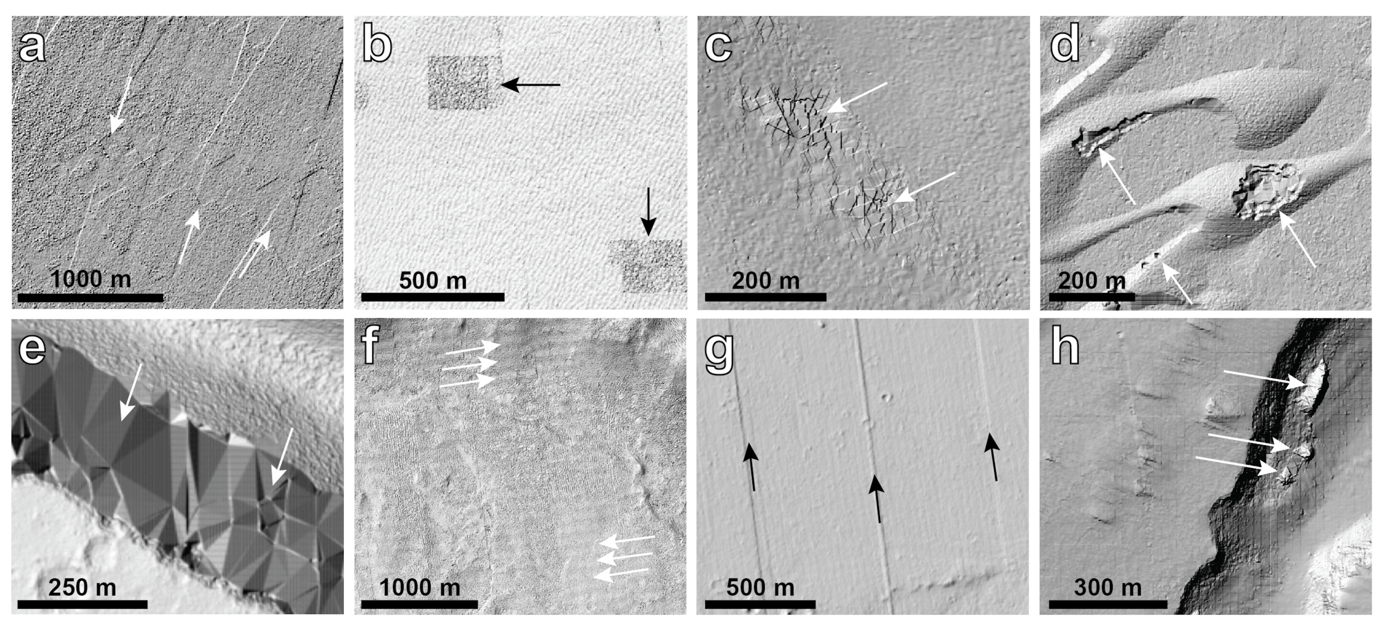
2.3.3. Noise, and Its Effect on Slope Maps

In some scientific applications, as well as landing site selection and surface operations planning, the absolute elevation measurements themselves are less important than their first derivative, which provides estimates of local slope angle and aspect. For example, the interpretation of enigmatic features called recurring slope lineae (RSL; Section 3.1) depends critically on how the growth of these features responds to slope angle and to what extent particular slope aspects favor their formation. Despite the high precision of HiRISE DTMs (Section 2.3.1), low-amplitude but short-wavelength noise characteristic of NGATE (Figure 10b) has an outsized effect on these first-derivative calculations. It is important to note that the error is not like a normal distribution of random noise applied to individual pixels. There may be systematic corrugations or patterns, or localized characteristic pits or spikes at a scale of a few meters. The relevance of identifying systematic artifacts is to understand the scales at which reliable slope estimates can be derived.

Slopes are substantially overestimated at the shortest baseline in the NGATE product [47]. This effect was mitigated in a study of RSL at Tivat crater by applying a two-step smoothing procedure to the 1 m/px DTM [58]. In the first step, they downsampled the DTM to 2 m/px using bicubic interpolation. In the second step, they applied a circular mean filter with 10 px (20 m) diameter to the downsampled DTM. This procedure removed a washboard-like noise in the HiRISE DTM, with ∼2 m amplitude and ∼8–10 m wavelength. In an earlier RSL study, Ref. [59] calculated RSL slopes over 20 m baselines and took the median of five overlapping profiles. RSL slopes were generally consistent between [58,59].

More recently, Ref. [47] showed that smoothing DTMs reduces errors but worsens resolution for Mars DTMs produced with a variety of software. Smoothing using one AATE pass in SOCET Set, or a 5 × 5 lowpass filter, can produce near-optimal results. Even so, slopes are consistently overestimated by ∼1${}^{°}$. Such an overestimate would have a larger relative effect on analysis of smooth terrains, but for landing site hazard characterization, a conservative estimation of slopes is preferable to an underestimation. Therefore, the optimal combination is to perform a modest amount of smoothing along with measuring slopes over a baseline that is somewhat larger than the effective resolution of the DTM [47].

Based on these studies, and on tests over a variety of DTMs of various surface types, a standardized slope map is in development at HiROC for release as a PDS Extra. The slope map will display a range of slope increments in degrees, taken over baselines of ∼9 m for a 1 m DTM. A possible set of ranges may include 0${}^{°}$–5${}^{°}$ (smooth), 5${}^{°}$–15${}^{°}$ and 15${}^{°}$–25${}^{°}$ for assessing exploration hazards, 25${}^{°}$–35${}^{°}$ for slopes within the angle of repose for unconsolidated granular material, and everything steeper than 35${}^{°}$ (Figure 12).

3. Change Detection Studies

The capability to resolve meter-scale features in HiRISE images, along with repeated imaging over the same target, has enabled unambiguous observations of surface changes on Mars. HiRISE DTMs are the best and often only way to get accurate slope and height estimates at high resolution from existing Mars datasets. Many types of surface changes have been observed by comparing HiRISE RDRs acquired at different times (e.g., [10,60,61,62,63]. Although a large number of sites can be qualitatively assessed using the RDRs, aligning images manually does not correct for differences in observation geometry, making visual comparisons challenging, especially on steep slopes. The RDRs are map projected onto a smoothed version of the MOLA global shape model [36], which can only provide topographic correction over the scale of features resolved by MOLA.

However, the qualitative identification of surface changes provides a starting point for selecting a smaller number of sites to focus on targeting with stereo pairs and additional images to generate one or more DTMs and the corresponding time series of orthorectified images [5,16,21,22,64,65]. These products, although time-consuming to produce, are necessary to make accurate and precise measurements of surface and volumetric changes on Mars. In the following sections, (Section 3.1–Section 3.4) we highlight studies of four types of surface processes that benefited from utilizing HiRISE DTMs and orthoimages to measure changes in a variety of landforms.

3.1. Recurring Slope Lineae

Recurring slope lineae (RSL) are linear markings on steep Martian slopes that are dark relative to their surroundings and that fade and then reappear in multiple Mars years [21]. They typically appear below bedrock outcrops and grow downslope over several months, usually when local temperatures are seasonally high [21,22,66,67]. Individual lineae are typically up to a few meters wide and can reach lengths of >1 km before growth ceases and they fade [66]. HiRISE images have confirmed repetition of this growth and fading cycle over multiple years at 86 sites [68,69]. The fundamental question is whether RSL are wet, perhaps trickles of liquid water or brine, or dry, such as grain flows of dust and/or sand [21,58,59,66,70,71]. If RSL are wet, the contemporary presence of liquid water at or near the surface would have significant implications for habitability, resources for human exploration, and our understanding of the Martian hydrosphere [72,73].

HiRISE is the only orbital imager that can resolve RSL that are on the order of a few meters wide; its stereo-derived products were instrumental in the discovery of RSL and have been essential to numerous RSL investigations. Several studies have used time series of orthoimages to characterize RSL growth rates and evaluate their compatibility with wet and dry models [58,65,67,74,75,76,77]. Ref. [59] used DTMs at ten sites to demonstrate that RSL terminate at slope angles similar to those of dune slipfaces, consistent with grain flow models. In similar analyses, Refs. [77,78] measured greater variability in terminal slope angles, but it is unclear to what extent noise intrinsic to the DTMs used may contribute to that variability (Section 2.3.3). Some measurements by [78] may not correspond to actual RSL [79]. Analysis of HiRISE topography revealed that many RSL originate near local topographic highs, unlikely locations for groundwater infiltration [65]. Using a DTM, Ref. [80] modeled the effects of a proposed dry RSL mechanism (a Knudsen pump) that is sensitive to both slope angle and aspect. Ref. [58] used a DTM to identify paired locations near and far from RSL with similar slope angles and aspects. Comparison of these locations in a time series of orthoimages revealed that RSL at the study site faded in two consecutive years because their surroundings darkened, not because the RSL themselves brightened. Such fading is most easily explained by widespread removal of bright dust, suggesting that RSL are likewise a dry phenomenon [58].

Monitoring of several key RSL locations has revealed episodic slumping of slope material [65,81]. These new slumps are larger in extent than nearby RSL, and deposit lobes with visible topographic expression, although the amount of relief is as yet below the resolution of HiRISE DTMs. Similar to RSL, the slumps are relatively darker than adjacent material and fade quickly (Figure S1). Mapping of newly observed and existing slumps on HiRISE DTMs shows that slumps initiate downslope of RSL, but where slopes still measure 25${}^{°}$–30${}^{°}$, and terminate where slopes decrease to 10${}^{°}$–20${}^{°}$ [81].

3.2. Aeolian Studies

As potentially active landforms, dunes and other bedforms are frequently targeted by HiRISE for both monitoring and stereo imaging. The first Mars aeolian study to extensively utilize an HiRISE DTM was [5], which quantified the migration rates, heights, and fluxes of sand dunes in Nili Patera (Figure 13). Critically, the geometrically corrected stereo orthoimages and DTM provided a consistent framework which could be input into the Co-registration of Optically Sensed Images and Correlation (COSI-Corr) tool suite [82]. The tool suite allows raw images to be registered to the stereo orthoimage using ground control points, which are to be optimized by the software allowing bedrock misregistration to be reduced down to less than an HiRISE pixel [83,84]. COSI-Corr was then used to generate a dense vectorial map of ripple displacements using annual or seasonal (non-stereo) images [5,83]. Collectively, these measurements showed that Nili Patera dunes were migrating near steady state and with sediment fluxes much lower than typical terrestrial examples. COSI-Corr allows sand ripple migration to be quantified with a precision of ∼1/3 of an HiRISE pixel (∼8 cm) using precise registration and cross-correlation between images [5]. Additional studies using HiRISE DTMs, orthoimages, and seasonal images have further applied COSI-Corr’s automatic co-registration to examine seasonal trends in ripple migration and, indirectly, local winds [83,84,85].

In certain locations with extremely active aeolian systems, dunes may have migrated beyond their original positions in early mission stereo pairs and DTMs. This may cause distortions if much later images are orthorectified over the original topography. For example, dunes could have migrated tens of meters during the multiple Mars years since acquiring the stereo pair for the DTM, resulting in steep slipfaces being projected over flat ground. In these cases, it is recommended that a new stereo pair be acquired with minimal time between acquisition of stereo halves to generate a DTM that accurately represents the current position of the dunes. Volumetric measurements of dunes, or of dune movement, are most reliable in locations where bedrock is exposed in the interdune areas.

More broadly, investigations using HiRISE DTMs have provided insight into Martian bedform morphology and dynamics. Active bedform heights, migration rates and sand fluxes each span two to three orders of magnitude across Mars [6,8,63,86,87,88,89,90]. Heights of migrating sand dunes vary widely (2–120 m tall), but most are 15–25 m tall. Global studies show that average dune migration rates converge around 0.5 m/yr (±0.4 m yr${}^{-1}$), dune crest fluxes average 7.8 ± 6.4 m${}^3$ m${}^{-1}$ yr${}^{-1}$, and the highest flux for an individual dune is 35 m${}^3$ m${}^{-1}$ yr${}^{-1}$ [89], where yr = 1 Earth year for all rates. Sand fluxes often are quite variable across a given dune field, where fluxes are lowest near the downwind portions of the field due to turbulence in the boundary layer related to local topography [5,90].

Bright bedforms termed megaripples, or small Transverse Aeolian Ridges (TARs), were generally thought to be static relics of past climates. Ref. [91] used long-baseline (4–5 Mars years) orthoimage pairs to show that TARs in Nili Fossae and within McLaughlin crater, with spacings of ∼1–35 m and heights of 0.8–2 m, are active today. More recently a systematic survey using long-baseline (4–7 Mars years) orthoimages found highly active megaripples at numerous locations within the north polar erg [85], challenging the previously held view that these landforms were last active during a past climate period with a thicker atmosphere [92,93,94,95].

3.3. Polar Features

Changes in polar features on Mars occur on both seasonal and inter-annual time scales. With the long duration of MRO’s mission, it is possible to use DTMs to quantify the effects and rates of seasonal processes and start to examine inter-annual variations on and near the polar ice deposits. We look at two types of features: south polar araneiforms (spider-like landforms) and small craters occurring in the north polar layered deposits.

South polar araneiforms. Radially branching networks that coalesce on a central depression have been dubbed “spiders” or araneiforms [96]. HiRISE observations of araneiforms across multiple seasons and years support the idea that dendritic channels are excavated by sublimation flows that become active beneath the seasonal transparent CO${}_2$ ice [97,98]. The scale of the seasonal features associated with araneiforms (fans, blotches, ice cracks) approaches the limits of the spatial resolution of HiRISE images, and the topographical data most relevant to studies of these seasonal polar phenomena come from HiRISE. DTMs are useful for the study of seasonal activity in more than one way. The most direct benefit is an improvement in the ability to directly compare observations from different local times, days, seasons and Mars years with the help of orthoimages, which remove ambiguities in image-to-image comparisons due to geometric distortions. At one site, informally named Inca City (81.4${}^{°}$ S, 295.6${}^{°}$ E), a monitoring campaign resulted in a series of 25 orthoimages spanning 5 Mars years. The Inca City time series has been analyzed for evidence of changes, growth, and measurable excavation of araneiforms. The time series orthoimages can be used to precisely measure meter-scale seasonal changes of frost and dust surface cover, which may indicate where volumetric changes are potentially occurring. Additionally, HiRISE DTMs provide important morphological measurements, such as slope and volume, which can be used to model the seasonal activity on the meter-scale level.

We demonstrate an analysis of two DTMs featuring araneiforms that were produced from stereo pairs taken during frost-free seasons in Mars Year (MY) [99] 30 and MY 32. The majority of systematic error seen in the difference map is due to jitter which appears as discontinuities at CCD boundaries (Figure 13a). The vertical precision of the DTMs places limits on the detection of real surface changes from erosion or other causes. EP is defined as the standard deviation of an individual height measurement in a DTM (Section 2.3), so the standard deviation of a height difference measurement equals the root summed square (RSS) of the EP values from both DTMs. The error distributions are only approximately Gaussian, so it is not possible to set exact bounds for statistical significance, but for a localized height difference to be considered significant it would have to be greater than a few times the standard deviation. At the location illustrated in Figure 14b, we compare the DTM differences to ±1 and 2 times the RSS EP, plotted about the local mean difference. In this case, all the differences between the DTMs fall within ±2 RSS EP, and most fall within ±1 RSS EP, indicating that they probably do not represent actual topographical changes in the araneiform. The use of the RSS EP illustrated here should be taken as a possible guideline, not as a strict rule. In particular, suspected topographical differences should be correlated with the geomorphic features seen in the images, regardless of where they fall within the RSS EP range.

Small north polar craters. Small craters found on the North Polar Layered Deposits (NPLD) are sites where preferential accumulation of water ice may occur in the shadowed crater interiors (e.g., [100]. If this is the case, then these craters are test sites where we can observe whether accumulation has occurred and therefore place constraints on realistic conditions useful for examining the hypothesis that the NPLD is gaining (or losing) mass. Constraining the current mass balance of water ice on Mars is a critical question to understanding the current climate and the recent history of surface water ice deposits on Mars (e.g., [101] and references therein). Of the fewer than 100 known small (<200 m diameter) NPLD craters [102,103], about 20 have bright deposits in their centers that persist through the north polar summer. These presumably water ice lenses offer the opportunity to measure changes in ice accumulation within craters that could be extrapolated to the surrounding surface.

Volume changes in the ice lenses must be calculated from multiple years of HiRISE images to distinguish long-term interannual variability from inter-seasonal variations due to events such as planet-encircling dust storms. Previous studies estimated ∼5 Mars years would be required to detect significant topographic changes, while a longer temporal baseline (i.e., a Martian decade) would allow the overall trend to be disentangled from interannual variability [103]. To accurately map changes in the ice lens of a given crater, images taken each Mars year at approximately the same time of year (solar longitude) are orthorectified to a DTM generated from an earlier stereo pair (Figure 15). Volume changes within the crater, measured from the DTM and follow-up images, are inputs to a model of ice accumulation or ablation conditions [104].

3.4. Gullies

Research on Martian gullies primarily deals with questions about their origin and present-day activity [15]. Because of their similarity to gullies carved by flowing liquid water on Earth, initial hypotheses were focused on resolving the problem of how to explain the presence of liquid water when the environmental conditions on Mars should not allow it [105,106]. Monitoring with the Mars Orbiter Camera (MOC) [107], Context Camera (CTX) [108] also on MRO, and HiRISE has shown that gullies are currently active, and that the driving process of present-day activity most likely involves the sublimation of CO${}_2$ frost and ice [13,61,109,110,111,112]. The earliest changes observed were attributed to liquid water [113]; however, ref. [114] used an HiRISE DTM to conduct flow modeling, which showed that the shape of one bright deposit was consistent with entirely dry flow. Ref. [115] modeled three new flows in gullies within Hale crater using an HiRISE DTM produced with methods similar to those described here and in [23] and found that they were consistent with either wet or CO${}_2$-gas fluidized flow. HiRISE DTMs have also played an important role in determining the 3D shapes of gullies and comparing them to those on Earth as a baseline for understanding the potential underlying processes [14,114,116,117,118]. Shadowing in gullies and changes in shadow position between stereo images cause artifacts in DTMs, often requiring manual editing [52]. Although the volumetric changes in gullies within craters have not yet been resolvable in HiRISE DTMs, the DTMs support the production of orthoimages which allow the surficial changes between images to be measured accurately (Figure 16).

In contrast to most gullies that are located on crater walls, gullies on dunes are active nearly every Mars year with broad-scale changes [61,119], suggesting their duration of activity is probably several hundreds of Mars years rather than the potential age of several millions of Mars years for gullies incised into rocky slopes [118,120,121]. As with other gullies, dune gullies are thought to be activated by the sublimation of CO${}_2$ ice, with springtime heating bringing the downslope movement of up to a few hundred cubic meters of sand within individual features [12,61,110,122]. While a few DTMs have been generated of very large dunes, such as a megabarchan dune in Kaiser crater (Figure 17) and the dense transverse dune field in Matara crater, in general, DTM generation over dark dunes can be problematic due to their low contrast and fine-scale changes over time.

4. Discussion

The ability of MRO and HiRISE to continue to acquire stereo and monitoring image sequences over progressively longer temporal baselines will increase the potential for understanding the rates of activity and evolving geologic processes. As highlighted in Section 3, some types of surface activity are readily observed by HiRISE as changes taking place over short time spans. Other types of surface activity on Mars may be occurring but have not been detected either due to a lack of sufficient stereo and/or repeated observations, or because the rate of activity is slower than what has been resolvable with orbital images. Examples of these active processes may include glacial movement or periglacial activity [123,124,125], changes at other icy deposits such as polar scarps [11] and mid-latitude ground ice exposures [64], mass wasting to estimate erosion rates [126] or evidence of seismicity from rock falls [127,128].

Methods and techniques developed for HiRISE-focused change detection studies can be extended to collaborative studies using other MRO data. However, observed surface changes tend to be best resolved in the HiRISE image sequences. The larger spatial coverage of CTX stereo is sometimes used to connect the HiRISE stereo images to the MOLA PEDR data. Other instruments on MRO, such as the Compact Reconnaissance Imaging Spectrometer for Mars (CRISM) [129], can be fused with HiRISE DTMs to correlate compositional information with stratigraphic contacts, layer thicknesses and orientations (e.g., [130,131,132,133,134,135,136,137,138]). Combined Shallow Radar (SHARAD) [139] and HiRISE studies have investigated the possibility of correlating stratigraphic layered exposures in HiRISE DTMs to SHARAD reflectors within the north polar layered deposits [140,141,142,143]. Ref. [144] correlated terraced crater morphology measured with HiRISE DTMs with SHARAD detections of subsurface reflectors to determine the presence of widespread deposits of excess ice (i.e., ice that is more than pore-filling) in Arcadia Planitia.

Photometric studies are another area that requires the precise orthorectification of images taken at a variety of illumination and phase angles. Topographic and atmospheric correction is required to derive photometric properties of the surface and measure the surface albedo accurately. HiRISE DTMs provide the geometric correction in the orthoimages, but arriving at an absolute atmospheric correction depends on having coordinated observations of the atmospheric properties. A scene-dependent relative correction can be performed by subtracting the brightness in a true shadowed area, if present. CRISM, which is boresight aligned with HiRISE, can provide useful data for atmospheric correction for HiRISE, but only for coordinated (simultaneous) observations, which are not available for most images [145].

Coordinated analyses with the Colour and Stereo Surface Imaging System (CaSSIS) [146] instrument on the European Space Agency’s Trace Gas Orbiter (TGO) [147] could expand the potential for photometric modeling of Mars’ surface [148] since TGO can image through all times-of-day. From the nominal 400 km altitude orbit of TGO, CaSSIS achieves a pixel scale of 4.6 m/px, which is smaller than that of CTX (5–6 m/px), but not as small as HiRISE (0.3 m/px). CaSSIS also has full swath width color filters that overlap the HiRISE bandpasses and an additional near infrared band [146]. The ability to acquire images at a wider range of illumination angles due to TGO having a non-Sun-synchronous orbit, comparable spatial resolution, and overlapping bandpasses make CaSSIS a complementary experiment to HiRISE investigations of surface activity, including RSL [149] and the structure of polar layered deposits [150]. HiRISE DTMs also provide a valuable reference dataset for the development of the CaSSIS DTM pipeline [55,151].

MRO and HiRISE data have been crucial for the science characterization and engineering assessment, mission planning, and visualization of potential exploration sites. Although landing site characterization with HiRISE data is described in detail in other places [23,53,152,153,154], it is worth mentioning here as many of the methods described in this paper have benefitted from the need to seamlessly merge multiple overlapping HiRISE DTMs with each other and with topographic data from other instruments, as well as from the methods of quality assessment developed for landing site characterization. HiRISE images and DTMs have proven critical for assessing hazards such as boulders (e.g., [23,155]) and steep slopes (e.g., [153]). HiRISE DTMs have also been used as reference datasets in the development and testing of innovative exploration technologies such as terrain relative navigation, which was successfully demonstrated by NASA’s Mars 2020 Perseverance rover [156,157,158].

Since becoming available in the PDS, HiRISE DTMs have been included in more than 800 refereed publications, with the number of papers generally increasing each year (Figure 18). Not all of the HiRISE DTMs used in these publications were derived using the methods described here. NASA Ames Research Center developed the Ames Stereo Pipeline (ASP) for use with stereo data from planetary as well as Earth-orbiting satellites [159]. ASP is a widely used tool for producing HiRISE DTMs and has the advantages that the software is free (Table A1), and the process is non-interactive and does not require extensive specialized training or hardware. One challenge with ASP is that orthorectifying additional images to an existing DTM requires a workflow outside of the standard automated process to create a DTM from a stereo pair. Moreover, interactive editing is not currently supported in ASP. While ASP is a powerful tool that makes DTM creation accessible to more researchers, some projects may require capabilities that only currently exist in SOCET Set. The increasing availability of these high-value products represents a benefit to the planetary science and engineering community. The availability of HiRISE DTMs and orthoimages in the PDS also provides opportunities for public engagement and visualization of the surface of Mars.

5. Conclusions

HiRISE images and stereo-derived topography provide the highest resolution data currently available from Mars’ orbit, and have enabled wide ranging discoveries about present-day geologic activity on the surface of Mars. HiRISE DTMs, created at 1 and 2-m horizontal post spacing and an estimated vertical precision of tens of cm and ∼1 m, respectively, enable precise geological measurements, the assessment of candidate landing sites, and visualization of landscapes on Mars. In this paper we described the methods used to create HiRISE DTMs and orthoimages, as well as sources of error, with the intention of providing users with an understanding of the potential, and limitations, of the data.

We describe the methods used to create additional HiRISE products that are critical to change detection studies on Mars, beyond the fundamental DTM. (1) In Section 2.2, we introduced the methods that are used to control additional images to an HiRISE DTM in a relative sense. Time series made up of such sequences of orthoimages have been used in many change detection studies, a few of which are highlighted in Section 3; (2) The same techniques can be applied to control another stereo pair over the same target to generate an additional DTM (Section 2.2.1) for the purpose of measuring volumetric changes; (3) The same methods are applied to control adjacent, overlapping HiRISE stereo pairs to create regional DTM mosaics (Section 2.2.2).

The effective resolution of any single HiRISE DTM depends on many factors including image quality, spacecraft jitter, and observation geometry, and should be assessed locally, particularly for understanding artifacts that may affect short-baseline slopes. In cases where the HiRISE stereo was controlled to MOLA, the absolute accuracy of the solution with respect to the MOLA global topography is on average within ±5 m vertically, and within 100 m horizontally, although it is often much better than these values. The precision of HiRISE orthoimage sequences is a consequence of the quality of their relative fit to the source stereo pair rather than the bundle adjustment to the global reference (MOLA). The relative precision of the orthoimage sequences is therefore much better than the absolute positional accuracy of the DTM. Systematic differences may exist between multi-temporal HiRISE DTMs, despite careful methods used to control them to a common reference. The user is therefore cautioned to consider the precision and accuracy of the individual DTMs, and to assess their local quality when measuring potential topographic changes, in part through the use of FOM maps. We provide a guideline that the magnitude of resolvable volumetric change must be larger than two times the root summed square (RSS) of the estimated vertical precision (EP) of the two DTMs, offset by any local systematic error (Figure 14). The use of HiRISE orthoimages sequences has been incredibly successful at monitoring and measuring planimetric surface changes over a variety of landforms, including dunes, gullies, and polar surfaces. Volumetric changes are measurable using multi-temporal HiRISE DTMs given that certain criteria are met, such as the existence of HiRISE stereo pairs before and after the changes, a long enough temporal baseline to make reliable observations of topographic changes, and a large enough geomporphic magnitude of change to be resolvable in the difference of HiRISE DTMs.

The methods described here have been developed and refined over many years through collaborative efforts across multiple institutions. The ISIS/SOCET Set workflow is not the only process available to create HiRISE DTMs, but it was used for all the DTMs that have been made available in the PDS archive. Although the resolution, quality, and accuracy of HiRISE DTMs are unprecedented in planetary datasets, the difficulty of the workflow described here presents a tradeoff between interactive and automated processes in terms of time and quality. This tradeoff has resulted in only a fraction of the thousands of acquired HiRISE stereo pairs being made into high quality DTMs so far, which has restricted studies of active processes to relatively few sites. Future development efforts by the HiRISE team will be focused on automating the orthorectification procedure as much as possible, particularly for sequences of monitoring images over existing stereo targets. As of 2021, MRO has continued to operate for more than sixteen years, and has ample fuel for more than ten additional years of operations. However, there are multiple risks to both the spacecraft and the instruments as they age. As HiRISE ages, degradation of the instrument may lead to the need to acquire more binned images in future years, which may reduce the opportunities to make the highest resolution (1 m GSD) DTMs. The importance of maintaining the continuity of monitoring active processes on Mars with high-resolution orbital cameras is analogous to the need for long-term continuous Earth satellite imaging for studies of global ecological systems (e.g., Landsat; [160]). Not only do these data expand our understanding of active surface processes on Mars, but they are also necessary to support current and future exploration.

References

1. Zurek, R.W.; Smrekar, S.E. An overview of the Mars Reconnaissance Orbiter (MRO) science mission. J. Geophys. Res. E Planets 2007, 112, 1–22. [Google Scholar] [CrossRef] [Green Version]
2. Diniega, S.; Bramson, A.M.; Buratti, B.; Buhler, P.; Burr, D.M.; Chojnacki, M.; Conway, S.J.; Dundas, C.M.; Hansen, C.J.; McEwen, A.S.; et al. Modern Mars’ geomorphological activity, driven by wind, frost, and gravity. Geomorphology 2021, 380, 107627. [Google Scholar] [CrossRef]
3. Dundas, C.M.; Becerra, P.; Byrne, S.; Chojnacki, M.; Daubar, I.J.; Diniega, S.; Hansen, C.J.; Herkenhoff, K.E.; Landis, M.E.; McEwen, A.S.; et al. Active Mars: A dynamic world. J. Geophys. Res. 2021, 126, e2021JE006876. [Google Scholar] [CrossRef]
4. Bridges, N.; Bourke, M.; Geissler, P.; Banks, M.; Colon, C.; Diniega, S.; Golombek, M.; Hansen, C.; Mattson, S.; McEwen, A.; et al. Planet-wide sand motion on Mars. Geology 2012, 40, 31–34. [Google Scholar] [CrossRef]
5. Bridges, N.T.; Ayoub, F.; Avouac, J.P.; Leprince, S.; Lucas, A.; Mattson, S. Earth-like sand fluxes on Mars. Nature 2012, 485, 339–342. [Google Scholar] [CrossRef] [PubMed] [Green Version]
6. Bridges, N.; Geissler, P.; Silvestro, S.; Banks, M. Bedform migration on Mars: Current results and future plans. Aeolian Res. 2013, 9, 133–151. [Google Scholar] [CrossRef]
7. Vaz, D.A.; Silvestro, S. Mapping and characterization of small-scale aeolian structures on Mars: An example from the MSL landing site in Gale Crater. Icarus 2014, 230, 151–161. [Google Scholar] [CrossRef]
8. Chojnacki, M.; Urso, A.; Fenton, L.K.; Michaels, T.I. Aeolian dune sediment flux heterogeneity in Meridiani Planum, Mars. Aeolian Res. 2017, 26, 73–88. [Google Scholar] [CrossRef] [Green Version]
9. Russell, P.; Thomas, N.; Byrne, S.; Herkenhoff, K.; Fishbaugh, K.; Bridges, N.; Okubo, C.; Milazzo, M.; Daubar, I.; Hansen, C.; et al. Seasonally active frost-dust avalanches on a north polar scarp of Mars captured by HiRISE. Geophys. Res. Lett. 2008, 35. [Google Scholar] [CrossRef]
10. Hansen, C.J.; Byrne, S.; Portyankina, G.; Bourke, M.; Dundas, C.; McEwen, A.; Mellon, M.; Pommerol, A.; Thomas, N. Observations of the northern seasonal polar cap on Mars: I. Spring sublimation activity and processes. Icarus 2013, 225, 881–897. [Google Scholar] [CrossRef]
11. Fanara, L.; Gwinner, K.; Hauber, E.; Oberst, J. Present-day erosion rate of north polar scarps on Mars due to active mass wasting. Icarus 2020, 342, 113434. [Google Scholar] [CrossRef]
12. Diniega, S.; Byrne, S.; Bridges, N.T.; Dundas, C.M.; McEwen, A.S. Seasonality of present-day Martian dune-gully activity. Geology 2010, 38, 1047–1050. [Google Scholar] [CrossRef] [Green Version]
13. Dundas, C.M.; McEwen, A.S.; Diniega, S.; Byrne, S.; Martinez-Alonso, S. New and recent gully activity on Mars as seen by HiRISE. Geophys. Res. Lett. 2010, 37. [Google Scholar] [CrossRef] [Green Version]
14. Kolb, K.J.; McEwen, A.S.; Pelletier, J.D. Investigating gully flow emplacement mechanisms using apex slopes. Icarus 2010, 208, 132–142. [Google Scholar] [CrossRef]
15. Conway, S.J.; de Haas, T.; Harrison, T.N. Martian gullies: A comprehensive review of observations, mechanisms and insights from Earth analogues. Geol. Soc. Lond. Spec. Publ. 2019, 467, 7–66. [Google Scholar] [CrossRef] [Green Version]
16. Dundas, C.M.; Byrne, S.; McEwen, A.S.; Mellon, M.T.; Kennedy, M.R.; Daubar, I.J.; Saper, L. HiRISE observations of new impact craters exposing Martian ground ice. J. Geophys. Res. Planets 2014, 119, 109–127. [Google Scholar] [CrossRef]
17. Daubar, I.J.; Dundas, C.M.; Byrne, S.; Geissler, P.; Bart, G.D.; McEwen, A.S.; Russell, P.S.; Chojnacki, M.; Golombek, M.P. Changes in blast zone albedo patterns around new Martian impact craters. Icarus 2016, 267, 86–105. [Google Scholar] [CrossRef]
18. Thomas, P.C.; James, P.B.; Calvin, W.M.; Haberle, R.; Malin, M.C. Residual south polar cap of Mars: Stratigraphy, history, and implications of recent changes. Icarus 2009, 203, 352–375. [Google Scholar] [CrossRef]
19. Becerra, P.; Byrne, S.; Brown, A.J. Transient bright “halos” on the south polar residual cap of Mars: Implications for mass-balance. Icarus 2015, 251, 211–225. [Google Scholar] [CrossRef]
20. Portyankina, G.; Hansen, C.J.; Aye, K.M. Present-day erosion of Martian polar terrain by the seasonal CO2 jets. Icarus 2017, 282, 93–103. [Google Scholar] [CrossRef]
21. McEwen, A.S.; Ojha, L.; Dundas, C.M.; Mattson, S.S.; Byrne, S.; Wray, J.J.; Cull, S.C.; Murchie, S.L.; Thomas, N.; Gulick, V.C. Seasonal flows on warm Martian slopes. Science 2011, 333, 740–743. [Google Scholar] [CrossRef] [PubMed] [Green Version]
22. Ojha, L.; McEwen, A.; Dundas, C.; Byrne, S.; Mattson, S.; Wray, J.; Masse, M.; Schaefer, E. HiRISE observations of recurring slope lineae (RSL) during southern summer on Mars. Icarus 2014, 231, 365–376. [Google Scholar] [CrossRef]
23. Kirk, R.L.; Howington-Kraus, E.; Rosiek, M.R.; Anderson, J.A.; Archinal, B.A.; Becker, K.J.; Cook, D.A.; Galuszka, D.M.; Geissler, P.E.; Hare, T.M.; et al. Ultrahigh resolution topographic mapping of Mars with MRO HiRISE stereo images: Meter-scale slopes of candidate Phoenix landing sites. J. Geophys. Res. 2008, 113, E00A24. [Google Scholar] [CrossRef]
24. Kirk, R.; Howington-Kraus, E.; Rosiek, M. Build your own topographic model: A photogrammetry guest facility for planetary researchers. In Proceedings of the 40th Lunar and Planetary Science Conference, The Woodlands, TX, USA, 23–27 March 2009. Abstract #1414. [Google Scholar]
25. Miller, S.B.; Walker, A.S. Further developments of Leica digital photogrammetric systems by Helava. In Proceedings of the ACSM ASPRS ANNUAL CONVENTION. American Soc Photogrammetry and Remote Sensing Amer Cong, New Orleans, LA, USA, 14–24 March 1993; Volume 3, p. 256. [Google Scholar]
26. Miller, S.B.; Walker, A.S. Die Entwicklung der digitalen photogrammetrischen Systeme von Leica und Helava. Z. Photogramm. Fernerkund. 1995, 63, 4–16. [Google Scholar]
27. BAE Systems. SOCET Set User’s Manual; Version 5.6.0; BAE Systems, Inc.: Falls Church, VA, USA, 2011. [Google Scholar]
28. Sides, S.C.; Becker, T.L.; Becker, K.J.; Edmundson, K.L.; Backer, J.W.; Wilson, T.J.; Weller, L.A.; Humphrey, I.R.; Berry, K.L.; Shepherd, M.R.; et al. The USGS Integrated Software for Imagers and Spectrometers (ISIS 3) instrument support, new capabilites, and releases. In Proceedings of the 48th Lunar and Planetary Science Conference, Houston, TX, USA, 20–24 March 2017; Volume 48. Abstract #2739.. [Google Scholar]
29. McEwen, A.S.; Eliason, E.M.; Bergstrom, J.W.; Bridges, N.T.; Hansen, C.J.; Delamere, W.A.; Grant, J.A.; Gulick, V.C.; Herkenhoff, K.E.; Keszthelyi, L.; et al. Mars Reconnaissance Orbiter’s High Resolution Imaging Science Experiment (HiRISE). J. Geophys. Res. 2007, 112, E05S02. [Google Scholar] [CrossRef] [Green Version]
30. Dorn, D.A.; Meiers, W.; Burkepile, J.; Freymiller, E.D.; Delamere, A.W.; McEwen, A.S.; Maggs, P.; Pool, P.J.; Wallace, I. HiRISE focal plane for use on the Mars Reconnaissance Orbiter. In Focal Plane Arrays for Space Telescopes; Grycewicz, T.J., McCreight, C.R., Eds.; SPIE: Bellingham, WA, USA, 2004; Volume 5167, pp. 63–71. [Google Scholar] [CrossRef]
31. Delamere, W.A.; Tornabene, L.L.; McEwen, A.S.; Becker, K.; Bergstrom, J.W.; Bridges, N.T.; Eliason, E.M.; Gallagher, D.; Herkenhoff, K.E.; Keszthelyi, L.; et al. Color imaging of Mars by the High Resolution Imaging Science Experiment (HiRISE). Icarus 2010, 205, 38–52. [Google Scholar] [CrossRef]
32. McEwen, A. Future high-resolution orbital reconnaissance with MRO/HIRISE. In Proceedings of the 42nd COSPAR Scientific Assembly, Pasadena, CA, USA, 14–22 July 2018; Volume 42, p. B4-2. [Google Scholar]
33. McEwen, A.; Banks, M.; Baugh, N.; Becker, K.; Boyd, A.; Bergstrom, J.; Beyer, R.; Bortolini, E.; Bridges, N.; Byrne, S.; et al. The High Resolution Imaging Science Experiment (HiRISE) during MRO’s primary science phase (PSP). Icarus 2010, 205, 2–37. [Google Scholar] [CrossRef]
34. Becker, K.; Archinal, B.; Hare, T.; Kirk, R.; Howington-Kraus, E.; Robinson, M.; Rosiek, M. Criteria for automated identification of stereo image pairs. In Proceedings of the 46th Annual Lunar and Planetary Science Conference, The Woodlands, TX, USA, 16–20 March 2015. Abstract #2703. [Google Scholar]
35. Smith, D.E.; Zuber, M.T.; Frey, H.V.; Garvin, J.B.; Head, J.W.; Muhleman, D.O.; Pettengill, G.H.; Phillips, R.J.; Solomon, S.C.; Zwally, H.J.; et al. Mars Orbiter Laser Altimeter: Experiment summary after the first year of global mapping of Mars. J. Geophys. Res. 2001, 106, 23689. [Google Scholar] [CrossRef]
36. Eliason, E.; Castalia, B.; Mattson, S.; Heyd, R.; Becker, K.; Anderson, J.; Sides, S. Software Interface Specification for HiRISE Reduced Data Record Products, Version 1.3; Jet Propulsion Laboratory: Pasadena, CA, USA, 2012.
37. Becker, K.J.; Milazzo, M.P.; Delamere, W.A.; Herkenhoff, K.E.; Eliason, E.M.; Russell, P.S.; Keszthelyi, L.P.; McEwen, A.S. hical—The HiRISE radiometric calibration software developed within the ISIS3 planetary image processing suite. In U.S. Geological Survey Techniques and Methods; Book 7; U.S. Department of the Interior: Reston, VA, USA, 2021; Chapter 27. [Google Scholar] [CrossRef]
38. Sutton, S.S.; Boyd, A.K.; Kirk, R.L.; Cook, D.; Backer, J.W.; Fennema, A.; Heyd, R.; McEwen, A.S.; Mirchandani, S.D. Correcting spacecraft jitter in HiRISE images. In Planetary Remote Sensing and Mapping; Wu, B., Di, K., Oberst, J., Karachevtseva, I., Eds.; Taylor & Francis Group: London, UK, 2019; Chapter 8; pp. 91–106. [Google Scholar]
39. McCleese, D.J.; Schofield, J.T.; Taylor, F.W.; Calcutt, S.B.; Foote, M.C.; Kass, D.M.; Leovy, C.B.; Paige, D.A.; Read, P.L.; Zurek, R.W. Mars Climate Sounder: An investigation of thermal and water vapor structure, dust and condensate distributions in the atmosphere, and energy balance of the polar regions. J. Geophys. Res. 2007, 112, E05S06. [Google Scholar] [CrossRef] [Green Version]
40. Acton, C.H. Ancillary data services of NASA’s navigation and ancillary information facility. Planet. Space Sci. 1996, 44, 65–70. [Google Scholar] [CrossRef]
41. Konopliv, A.S.; Asmar, S.W.; Folkner, W.M.; Karatekin, Ö.; Nunes, D.C.; Smrekar, S.E.; Yoder, C.F.; Zuber, M.T. Mars high resolution gravity fields from MRO, Mars seasonal gravity, and other dynamical parameters. Icarus 2011, 211, 401–428. [Google Scholar] [CrossRef]
42. Konopliv, A.S.; Park, R.S.; Folkner, W.M. An improved JPL Mars gravity field and orientation from Mars orbiter and lander tracking data. Icarus 2016, 274, 253–260. [Google Scholar] [CrossRef]
43. Menon, P.; Wagner, S.; Demcak, S.; Jefferson, D.; Graat, E.; Lee, K.; Schulze, W. 50,000 laps around Mars: Navigating the Mars Reconnaissance Orbiter through the extended missions (January 2009–March 2017). In International Symposium on Space Flight Dynamics; Jet Propulsion Laboratory, National Aeronautics and Space Administration: Pasadena, CA, USA, 2017. [Google Scholar]
44. Zhang, B.; Miller, S.; Walker, S.; Devencia, K. Next Generation Automatic Terrain Extraction using Microsoft UltraCam imagery. In Proceedings of the ASPRS 2007 Annual Conference, Tampa, FL, USA, 7–11 May 2007. [Google Scholar]
45. Zhang, B.; Miller, S.K.D.; Walker, S. Automatic terrain extraction using multiple image pair and back matching. In Proceedings of the ASPRS 2006 Annual Conference, Reno, NV, USA, 1–5 May 2006. [Google Scholar]
46. Henriksen, M.; Manheim, M.; Burns, K.; Seymour, P.; Speyerer, E.; Deran, A.; Boyd, A.; Howington-Kraus, E.; Rosiek, M.; Archinal, B.; et al. Extracting accurate and precise topography from LROC narrow angle camera stereo observations. Icarus 2017, 283, 122–137. [Google Scholar] [CrossRef]
47. Kirk, R.; Mayer, D.; Redding, B.L.; Galuszka, D.; Fergason, R.; Hare, T.; Gwinner, K. Further adventures in Mars DTM quality: Smoothing errors, sharpening details. Remote Sens. 2021, 43, 659–666. [Google Scholar] [CrossRef]
48. Neumann, G.A.; Rowlands, D.D.; Lemoine, F.G.; Smith, D.E.; Zuber, M.T. Crossover analysis of Mars Orbiter Laser Altimeter data. J. Geophys. Res. E Planets 2001, 106, 23753–23768. [Google Scholar] [CrossRef] [Green Version]
49. Kilgallon, A.; Stephens, J.; Sutton, S.; Mueting, J. AutoTriangulation: A new tool for controlling stereo pairs to laser altimetry. In Proceedings of the 46th Lunar and Planetary Science Conference, The Woodlands, TX, USA, 16–20 March 2015. Abstract #2373. [Google Scholar]
50. Golombek, M.; Grant, J.; Kipp, D.; Vasavada, A.; Kirk, R.; Fergason, R.; Bellutta, P.; Calef, F.; Larsen, K.; Katayama, Y.; et al. Selection of the Mars Science Laboratory landing site. Space Sci. Rev. 2012, 170, 641–737. [Google Scholar] [CrossRef]
51. Sutton, S.; Heyd, R.; Fennema, A.; Mcewen, A.S.; Kirk, R.L.; Howington-Kraus, E.; Espinoza, A. HiRISE digital terrain models: Updates and advances. In Proceedings of the Second Planetary Data Workshop, Flagstaff, AZ, USA, 8–11 June 2015. Abstract #7056. [Google Scholar]
52. Sutton, S.S.; Chojnacki, M.; Kilgallon, A. Precision and accuracy of simultaneously collected HiRISE digital terrain models. In Proceedings of the 46th Lunar and Planetary Science Conference, The Woodlands, TX, USA, 16–20 March 2015. Abstract #3010. [Google Scholar]
53. Kirk, R.L.; Howington-Kraus, E.; Redding, B.; Galuszka, D.; Hare, T.M.; Archinal, B.A.; Soderblom, L.A.; Barrett, J.M. High-resolution topomapping of candidate MER landing sites with Mars Orbiter Camera narrow-angle images. J. Geophys. Res. 2003, 108, 8088. [Google Scholar] [CrossRef]
54. Cook, A.C.; Oberst, J.; Roatsch, T.; Jaumann, R.; Acton, C. Clementine imagery: Selenographic coverage for cartographic and scientific use. Planet. Space Sci. 1996, 44, 1135–1148. [Google Scholar] [CrossRef]
55. Simioni, E.; Re, C.; Mudric, T.; Cremonese, G.; Tulyakov, S.; Petrella, A.; Pommerol, A.; Thomas, N. 3DPD: A photogrammetric pipeline for a PUSH frame stereo cameras. Planet. Space Sci. 2021, 198, 105165. [Google Scholar] [CrossRef]
56. Heipke, C.; Oberst, J.; Albertz, J.; Attwenger, M.; Dorninger, P.; Dorrer, E.; Ewe, M.; Gehrke, S.; Gwinner, K.; Hirschmüller, H.; et al. Evaluating planetary digital terrain models–The HRSC DTM test. Planet. Space Sci. 2007, 55, 2173–2191. [Google Scholar] [CrossRef]
57. Mattson, S.; Russell, P.; Byrne, S.; Kirk, R.L.; Herkenhoff, K.; McEwen, A.S. Production and error analysis of polar digital terrain models from HiRISE. In Proceedings of the 43rd Lunar and Planetary Science Conference, Pasadena, CA, USA, 14–22 July 2012. Abstract #2659. [Google Scholar]
58. Schaefer, E.I.; McEwen, A.S.; Sutton, S.S. A case study of recurring slope lineae (RSL) at Tivat crater: Implications for RSL origins. Icarus 2019, 317, 621–648. [Google Scholar] [CrossRef]
59. Dundas, C.M.; McEwen, A.S.; Chojnacki, M.; Milazzo, M.P.; Byrne, S.; McElwaine, J.N.; Urso, A. Granular flows at recurring slope lineae on Mars indicate a limited role for liquid water. Nat. Geosci. 2017, 10, 903–907. [Google Scholar] [CrossRef] [Green Version]
60. Hansen, C.J.; Bourke, M.; Bridges, N.T.; Byrne, S.; Colon, C.; Diniega, S.; Dundas, C.; Herkenhoff, K.; McEwen, A.; Mellon, M.; et al. Seasonal erosion and restoration of Mars’ northern polar dunes. Science 2011, 331, 575–578. [Google Scholar] [CrossRef]
61. Dundas, C.M.; Diniega, S.; Hansen, C.J.; Byrne, S.; McEwen, A.S. Seasonal activity and morphological changes in Martian gullies. Icarus 2012, 220, 124–143. [Google Scholar] [CrossRef]
62. Dundas, C.M.; Mellon, M.T.; Conway, S.J.; Gastineau, R. Active boulder movement at high Martian latitudes. Geophys. Res. Lett. 2019, 46, 5075–5082. [Google Scholar] [CrossRef] [Green Version]
63. Banks, M.E.; Fenton, L.K.; Bridges, N.T.; Geissler, P.E.; Chojnacki, M.; Runyon, K.D.; Silvestro, S.; Zimbelman, J.R. Patterns in mobility and modification of middle- and high-latitude southern hemisphere dunes on Mars. J. Geophys. Res. Planets 2018, 123, 3205–3219. [Google Scholar] [CrossRef] [Green Version]
64. Dundas, C.M.; Bramson, A.M.; Ojha, L.; Wray, J.J.; Mellon, M.T.; Byrne, S.; McEwen, A.S.; Putzig, N.E.; Viola, D.; Sutton, S.; et al. Exposed subsurface ice sheets in the Martian mid-latitudes. Science 2018, 359, 199–201. [Google Scholar] [CrossRef] [Green Version]
65. Chojnacki, M.; McEwen, A.; Dundas, C.; Ojha, L.; Urso, A.; Sutton, S. Geologic context of recurring slope lineae in Melas and Coprates Chasmata, Mars. J. Geophys. Res. Planets 2016, 121, 1204–1231. [Google Scholar] [CrossRef] [Green Version]
66. McEwen, A.S.; Dundas, C.M.; Mattson, S.S.; Toigo, A.D.; Ojha, L.; Wray, J.J.; Chojnacki, M.; Byrne, S.; Murchie, S.L.; Thomas, N. Recurring slope lineae in equatorial regions of Mars. Nat. Geosci. 2013, 7, 53–58. [Google Scholar] [CrossRef]
67. Stillman, D.E.; Michaels, T.I.; Grimm, R.E.; Hanley, J. Observations and modeling of northern mid-latitude recurring slope lineae (RSL) suggest recharge by a present-day Martian briny aquifer. Icarus 2016, 265, 125–138. [Google Scholar] [CrossRef]
68. Stillman, D.E.; Michaels, T.I.; Grimm, R.E. Characteristics of the numerous and widespread recurring slope lineae (RSL) in Valles Marineris, Mars. Icarus 2017, 285, 195–210. [Google Scholar] [CrossRef]
69. Stillman, D.E.; Grimm, R.E. Two pulses of seasonal activity in Martian southern mid-latitude recurring slope lineae (RSL). Icarus 2018, 302, 126–133. [Google Scholar] [CrossRef]
70. McEwen, A.S.; Schaefer, E.I.; Dundas, C.M.; Sutton, S.S.; Tamppari, L.K.; Chojnacki, M. Mars: Abundant recurring slope lineae (RSL) following the planet-encircling dust event (PEDE) of 2018. J. Geophys. Res. Planets 2021, 126, e2020JE006575. [Google Scholar] [CrossRef]
71. Millot, C.; Quantin-Nataf, C.; Leyrat, C.; Enjolras, M. Local topography effects on the surface temperatures on Mars—Application to the case of recurring slope lineae (RSL). Icarus 2021, 355, 114136. [Google Scholar] [CrossRef]
72. Grimm, R.E.; Harrison, K.P.; Stillman, D.E.; Kirchoff, M.R. On the secular retention of ground water and ice on Mars. J. Geophys. Res. Planets 2017, 122, 94–109. [Google Scholar] [CrossRef]
73. McEwen, A.S. Are recurring slope lineae habitable? In From Habitability to Life on Mars; Elsevier: Amsterdam, The Netherlands, 2018; pp. 249–274. [Google Scholar] [CrossRef]
74. Grimm, R.E.; Harrison, K.P.; Stillman, D.E. Water budgets of Martian recurring slope lineae. Icarus 2014, 233, 316–327. [Google Scholar] [CrossRef]
75. Levy, J. Hydrological characteristics of recurrent slope lineae on Mars: Evidence for liquid flow through regolith and comparisons with Antarctic terrestrial analogs. Icarus 2012, 219, 1–4. [Google Scholar] [CrossRef]
76. Stillman, D.E.; Michaels, T.I.; Grimm, R.E.; Harrison, K.P. New observations of Martian southern mid-latitude recurring slope lineae (RSL) imply formation by freshwater subsurface flows. Icarus 2014, 233, 328–341. [Google Scholar] [CrossRef]
77. Stillman, D.E.; Bue, B.D.; Wagstaff, K.L.; Primm, K.M.; Michaels, T.I.; Grimm, R.E. Evaluation of wet and dry recurring slope lineae (RSL) formation mechanisms based on quantitative mapping of RSL in Garni Crater, Valles Marineris, Mars. Icarus 2020, 335, 113420. [Google Scholar] [CrossRef]
78. Tebolt, M.; Levy, J.; Goudge, T.; Schorghofer, N. Slope, elevation, and thermal inertia trends of Martian recurring slope lineae initiation and termination points: Multiple possible processes occurring on coarse, sandy slopes. Icarus 2020, 338, 113536. [Google Scholar] [CrossRef]
79. Dundas, C.M. An aeolian grainflow model for Martian recurring slope lineae. Icarus 2020, 343, 113681. [Google Scholar] [CrossRef] [PubMed]
80. Schmidt, F.; Andrieu, F.; Costard, F.; Kocifaj, M.; Meresescu, A.G. Formation of recurring slope lineae on Mars by rarefied gas-triggered granular flows. Nat. Geosci. 2017, 10, 270–273. [Google Scholar] [CrossRef]
81. Ojha, L.; Chojnacki, M.; McDonald, G.D.; Shumway, A.; Wolff, M.J.; Smith, M.D.; McEwen, A.S.; Ferrier, K.; Huber, C.; Wray, J.J.; et al. Seasonal slumps in Juventae Chasma, Mars. J. Geophys. Res. Planets 2017, 122, 2193–2214. [Google Scholar] [CrossRef] [Green Version]
82. Leprince, S.; Barbot, S.; Ayoub, F.; Avouac, J.P. Automatic and precise orthorectification, coregistration, and subpixel correlation of satellite images, application to ground deformation measurements. IEEE Trans. Geosci. Remote Sens. 2007, 45, 1529–1558. [Google Scholar] [CrossRef] [Green Version]
83. Ayoub, F.; Avouac, J.P.; Newman, C.E.; Richardson, M.I.; Lucas, A.; Leprince, S.; Bridges, N.T. Threshold for sand mobility on Mars calibrated from seasonal variations of sand flux. Nat. Commun. 2014, 5, 1–8. [Google Scholar] [CrossRef] [Green Version]
84. Roback, K.P.; Runyon, K.; Newman, C.; Avouac, J.P. Multi-year measurements of ripple and dune migration on Mars: Implications for the wind regime and sand transport. Icarus 2022, 380, 114966. [Google Scholar] [CrossRef]
85. Chojnacki, M.; Vaz, D.A.; Silvestro, S.; Silva, D.C.A. Widespread megaripple activity across the north polar ergs of Mars. J. Geophys. Res. Planets 2021, 126, 1–19. [Google Scholar] [CrossRef]
86. Bridges, N.T.; Sullivan, R.; Newman, C.E.; Navarro, S.; van Beek, J.; Ewing, R.C.; Ayoub, F.; Silvestro, S.; Gasnault, O.; Le Mouélic, S.; et al. Martian aeolian activity at the Bagnold Dunes, Gale Crater: The view from the surface and orbit. J. Geophys. Res. Planets 2017, 122, 2077–2110. [Google Scholar] [CrossRef]
87. Chojnacki, M.; Johnson, J.R.; Moersch, J.E.; Fenton, L.K.; Michaels, T.I.; Bell, J.F. Persistent aeolian activity at Endeavour crater, Meridiani Planum, Mars: New observations from orbit and the surface. Icarus 2015, 251, 275–290. [Google Scholar] [CrossRef]
88. Chojnacki, M.; Banks, M.; Urso, A. Wind-driven erosion and exposure potential at Mars 2020 rover candidate-landing Sites. J. Geophys. Res. Planets 2018, 123, 468–488. [Google Scholar] [CrossRef]
89. Chojnacki, M.; Banks, M.E.; Fenton, L.K.; Urso, A.C. Boundary condition controls on the high-sand-flux regions of Mars. Geology 2019, 47, 427–430. [Google Scholar] [CrossRef]
90. Runyon, K.; Bridges, N.; Ayoub, F.; Newman, C.; Quade, J. An integrated model for dune morphology and sand fluxes on Mars. Earth Planet. Sci. Lett. 2017, 457, 204–212. [Google Scholar] [CrossRef]
91. Silvestro, S.; Chojnacki, M.; Vaz, D.A.; Cardinale, M.; Yizhaq, H.; Esposito, F. Megaripple migration on Mars. J. Geophys. Res. Planets 2020, 125. [Google Scholar] [CrossRef]
92. Golombek, M.; Robinson, K.; McEwen, A.; Bridges, N.; Ivanov, B.; Tornabene, L.; Sullivan, R. Constraints on ripple migration at Meridiani Planum from Opportunity and HiRISE observations of fresh craters. J. Geophys. Res. Planets 2010, 115, E00F08. [Google Scholar] [CrossRef] [Green Version]
93. Balme, M.; Berman, D.C.; Bourke, M.C.; Zimbelman, J.R. Transverse aeolian ridges (TARs) on Mars. Geomorphology 2008, 101, 703–720. [Google Scholar] [CrossRef] [Green Version]
94. Berman, D.C.; Balme, M.R.; Rafkin, S.C.; Zimbelman, J.R. Transverse aeolian ridges (TARs) on Mars II: Distributions, orientations, and ages. Icarus 2011, 213, 116–130. [Google Scholar] [CrossRef]
95. Berman, D.C.; Balme, M.R.; Michalski, J.R.; Clark, S.C.; Joseph, E.C.S. High-resolution investigations of transverse aeolian ridges on Mars. Icarus 2018, 312, 247–266. [Google Scholar] [CrossRef] [Green Version]
96. Piqueux, S.; Byrne, S.; Richardson, M.I. Sublimation of Mars’s southern seasonal CO2 ice cap and the formation of spiders. J. Geophys. Res. Planets 2003, 108. [Google Scholar] [CrossRef] [Green Version]
97. Kieffer, H.H. Cold jets in the Martian polar caps. J. Geophys. Res. Planets 2007, 112. [Google Scholar] [CrossRef] [Green Version]
98. Portyankina, G.; Markiewicz, W.J.; Thomas, N.; Hansen, C.J.; Milazzo, M. HiRISE observations of gas sublimation-driven activity in Mars’ southern polar regions: III. Models of processes involving translucent ice. Icarus 2010, 205, 311–320. [Google Scholar] [CrossRef]
99. Piqueux, S.; Byrne, S.; Kieffer, H.H.; Titus, T.N.; Hansen, C.J. Enumeration of Mars years and seasons since the beginning of telescopic exploration. Icarus 2015, 251, 332–338. [Google Scholar] [CrossRef]
100. Ingersoll, A.P.; Svitek, T.; Murray, B.C. Stability of polar frosts in spherical bowl-shaped craters on the Moon, Mercury, and Mars. Icarus 1992, 100, 40–47. [Google Scholar] [CrossRef]
101. Smith, I.B.; Hayne, P.O.; Byrne, S.; Becerra, P.; Kahre, M.; Calvin, W.; Hvidberg, C.; Milkovich, S.; Buhler, P.; Landis, M.; et al. The Holy Grail: A road map for unlocking the climate record stored within Mars’ polar layered deposits. Planet. Space Sci. 2020, 184, 104841. [Google Scholar] [CrossRef] [Green Version]
102. Banks, M.E.; Byrne, S.; Galla, K.; McEwen, A.S.; Bray, V.J.; Dundas, C.M.; Fishbaugh, K.E.; Herkenhoff, K.E.; Murray, B.C. Crater population and resurfacing of the Martian north polar layered deposits. J. Geophys. Res. E Planets 2010, 115, 1–11. [Google Scholar] [CrossRef] [Green Version]
103. Landis, M.; Byrne, S.; Daubar, I.; Herkenhoff, K.; Dundas, C. Surface age and resurfacing Rates of the north polar layered deposits, Mars. In Proceedings of the Sixth International Conference on Mars Polar Science and Exploration, Reykjavik, Iceland, 5–9 September 2016; Volume 1926. LPI Contributions Abstract #6013.. [Google Scholar]
104. Landis, M.; Byrne, S.; Hayne, P.; Piqueux, S.; Wilcoski, A. Interannual variability of ice within north polar layered deposits craters on Mars. In Proceedings of the 52nd Lunar and Planetary Science Conference, The Woodlands, TX, USA, 15–19 March 2021. Abstract #1653. [Google Scholar]
105. Malin, M.C.; Edgett, K.S. Evidence for recent groundwater seepage and surface runoff on Mars. Science 2000, 288, 2330–2335. [Google Scholar] [CrossRef] [Green Version]
106. Costard, F.; Forget, F.; Mangold, N.; Peulvast, J.P. Formation of recent Martian debris flows by melting of near-surface ground ice at high obliquity. Science 2002, 295, 110–113. [Google Scholar] [CrossRef] [Green Version]
107. Malin, M.C.; Danielson, G.E.; Ingersoll, A.P.; Masursky, H.; Veverka, J.; Ravine, M.A.; Soulanille, T.A. Mars Observer camera. J. Geophys. Res. Planets 1992, 97, 7699–7718. [Google Scholar] [CrossRef]
108. Malin, M.C.; Bell, J.F.; Cantor, B.A.; Caplinger, M.A.; Calvin, W.M.; Clancy, R.T.; Edgett, K.S.; Edwards, L.; Haberle, R.M.; James, P.B.; et al. Context Camera Investigation on board the Mars Reconnaissance Orbiter. J. Geophys. Res. 2007, 112, E05S04. [Google Scholar] [CrossRef] [Green Version]
109. Diniega, S.; Hansen, C.; McElwaine, J.; Hugenholtz, C.; Dundas, C.; McEwen, A.; Bourke, M. A new dry hypothesis for the formation of Martian linear gullies. Icarus 2013, 225, 526–537. [Google Scholar] [CrossRef]
110. Pasquon, K.; Gargani, J.; Massé, M.; Vincendon, M.; Conway, S.J.; Séjourné, A.; Jomelli, V.; Balme, M.R.; Lopez, S.; Guimpier, A. Present-day development of gully-channel sinuosity by carbon dioxide gas supported flows on Mars. Icarus 2019, 329, 296–313. [Google Scholar] [CrossRef]
111. Raack, J.; Reiss, D.; Appéré, T.; Vincendon, M.; Ruesch, O.; Hiesinger, H. Present-day seasonal gully activity in a south polar pit (Sisyphi Cavi) on Mars. Icarus 2015, 251, 226–243. [Google Scholar] [CrossRef]
112. Raack, J.; Conway, S.J.; Heyer, T.; Bickel, V.T.; Philippe, M.; Hiesinger, H.; Johnsson, A.; Mass, M. Present-day gully activity in Sisyphi Cavi, Mars—Flow-like features and block movements. Icarus 2020, 350, 113899. [Google Scholar] [CrossRef]
113. Malin, M.; Edgett, K.; Posiolova, L.; Mccolley, S.; Noe Dobrea, E. Present-day impact cratering rate and contemporary gully activity on Mars. Science 2006, 314, 1573–1577. [Google Scholar] [CrossRef]
114. Pelletier, J.D.; Kolb, K.J.; McEwen, A.S.; Kirk, R.L. Recent bright gully deposits on Mars: Wet or dry flow? Geology 2008, 36, 211–214. [Google Scholar] [CrossRef]
115. De Haas, T.; McArdell, B.W.; Conway, S.J.; McElwaine, J.N.; Kleinhans, M.G.; Salese, F.; Grindrod, P.M. Initiation and flow conditions of contemporary flows in Martian gullies. J. Geophys. Res. Planets 2019, 124, 2246–2271. [Google Scholar] [CrossRef] [Green Version]
116. Conway, S.J.; Balme, M.R.; Murray, J.B.; Towner, M.C.; Okubo, C.H.; Grindrod, P.M. The indication of Martian gully formation processes by slope—Area analysis. Geol. Soc. Lond. Spec. Publ. 2011, 356, 171–201. [Google Scholar] [CrossRef] [Green Version]
117. Conway, S.J.; Balme, M.R. A novel topographic parameterization scheme indicates that Martian gullies display the signature of liquid water. Earth Planet. Sci. Lett. 2016, 454, 36–45. [Google Scholar] [CrossRef] [Green Version]
118. De Haas, T.; Conway, S.J.; Butcher, F.E.G.; Levy, J.; Grindrod, P.M.; Goudge, T.A.; Balme, M.R. Time will tell: Temporal evolution of Martian gullies and palaeoclimatic implications. Geol. Soc. Lond. Spec. Publ. 2019, 467, 165–186. [Google Scholar] [CrossRef]
119. Dundas, C.M.; Diniega, S.; McEwen, A.S. Long-term monitoring of Martian gully formation and evolution with MRO/HiRISE. Icarus 2015, 251, 244–263. [Google Scholar] [CrossRef]
120. Reiss, D.; Van Gasselt, S.; Neukum, G.; Jaumann, R. Absolute dune ages and implications for the time of formation of gullies in Nirgal Vallis, Mars. J. Geophys. Res. Planets 2004, 109, E06007. [Google Scholar] [CrossRef] [Green Version]
121. Schon, S.C.; Head, J.W.; Fassett, C.I. Unique chronostratigraphic marker in depositional fan stratigraphy on Mars: Evidence for ca. 1.25 Ma gully activity and surficial meltwater origin. Geology 2009, 37, 207–210. [Google Scholar] [CrossRef]
122. Sylvest, M.E.; Dixon, J.C.; Conway, S.J.; Patel, M.R.; McElwaine, J.N.; Hagermann, A.; Barnes, A. CO2 sublimation in Martian gullies: Laboratory experiments at varied slope angle and regolith grain sizes. Geol. Soc. Lond. Spec. Publ. 2019, 467, 343–371. [Google Scholar] [CrossRef]
123. Head, J.W.; Neukum, G.; Jaumann, R.; Hiesinger, H.; Hauber, E.; Carr, M.; Masson, P.; Foing, B.; Hoffmann, H.; Kreslavsky, M.; et al. Tropical to mid-latitude snow and ice accumulation, flow and glaciation on Mars. Nature 2005, 434, 346–351. [Google Scholar] [CrossRef]
124. Sori, M.M.; Byrne, S.; Hamilton, C.W.; Landis, M.E. Viscous flow rates of icy topography on the north polar layered deposits of Mars. Geophys. Res. Lett. 2016, 43, 541–549. [Google Scholar] [CrossRef] [Green Version]
125. Sori, M.M.; Byrne, S.; Bramson, A.M. Present-day flow rates of mid-latitude glaciers on Mars. Eur. Planet. Sci. Congr. 2017, 11, 1–2, Abstract #382. [Google Scholar]
126. Thomas, M.F.; McEwen, A.S.; Dundas, C.M. Present-day mass wasting in sulfate-rich sediments in the equatorial regions of Mars. Icarus 2020, 342, 113566. [Google Scholar] [CrossRef]
127. Roberts, G.P.; Matthews, B.; Bristow, C.; Guerrieri, L.; Vetterlein, J. Possible evidence of paleomarsquakes from fallen boulder populations, Cerberus Fossae, Mars. J. Geophys. Res. Planets 2012, 117, E02009. [Google Scholar] [CrossRef] [Green Version]
128. Grindrod, P.M.; Hollingsworth, J.; Ayoub, F.; Hunt, S.A. The search for active Marsquakes using subpixel coregistration and correlation: Best practice and first results. J. Geophys. Res. Planets 2018, 123, 1881–1900. [Google Scholar] [CrossRef]
129. Murchie, S.; Arvidson, R.; Bedini, P.; Beisser, K.; Bibring, J.P.; Bishop, J.; Boldt, J.; Cavender, P.; Choo, T.; Clancy, R.T.; et al. Compact Reconnaissance Imaging Spectrometer for Mars (CRISM) on Mars Reconnaissance Orbiter (MRO). J. Geophys. Res. 2007, 112, E05S03. [Google Scholar] [CrossRef]
130. Wray, J.J.; Ehlmann, B.L.; Squyres, S.W.; Mustard, J.F.; Kirk, R.L. Compositional stratigraphy of clay-bearing layered deposits at Mawrth Vallis, Mars. Geophys. Res. Lett. 2008, 35, L12202. [Google Scholar] [CrossRef] [Green Version]
131. Wray, J.J.; Milliken, R.E.; Dundas, C.M.; Swayze, G.A.; Andrews-Hanna, J.C.; Baldridge, A.M.; Chojnacki, M.; Bishop, J.L.; Ehlmann, B.L.; Murchie, S.L.; et al. Columbus crater and other possible groundwater-fed paleolakes of Terra Sirenum, Mars. J. Geophys. Res. E Planets 2011, 116, 1–41. [Google Scholar] [CrossRef] [Green Version]
132. Weitz, C.M.; Milliken, R.E.; Grant, J.A.; McEwen, A.S.; Williams, R.M.E.; Bishop, J.L.; Thomson, B.J. Mars Reconnaissance Orbiter observations of light-toned layered deposits and associated fluvial landforms on the plateaus adjacent to Valles Marineris. Icarus 2010, 205, 73–102. [Google Scholar] [CrossRef]
133. Weitz, C.M.; Bishop, J.L.; Thollot, P.; Mangold, N.; Roach, L.H. Diverse mineralogies in two troughs of Noctis Labyrinthus, Mars. Geology 2011, 39, 899–902. [Google Scholar] [CrossRef]
134. Weitz, C.M.; Noe Dobrea, E.Z.; Lane, M.D.; Knudson, A.T. Geologic relationships between gray hematite, sulfates, and clays in Capri Chasma. J. Geophys. Res. Planets 2012, 117, E00J09. [Google Scholar] [CrossRef]
135. Okubo, C.H. Structural geology of Amazonian-aged layered sedimentary deposits in southwest Candor Chasma, Mars. Icarus 2010, 207, 210–225. [Google Scholar] [CrossRef]
136. Tirsch, D.; Bishop, J.L.; Voigt, J.R.C.; Tornabene, L.L.; Erkeling, G.; Jaumann, R. Geology of central Libya Montes, Mars: Aqueous alteration history from mineralogical and morphological mapping. Icarus 2018, 314, 12–34. [Google Scholar] [CrossRef] [Green Version]
137. Tornabene, L.L.; Seelos, F.P.; Pommerol, A.; Thomas, N.; Caudill, C.M.; Becerra, P.; Bridges, J.C.; Byrne, S.; Cardinale, M.; Chojnacki, M.; et al. Image simulation and assessment of the colour and spatial capabilities of the Colour and Stereo Surface Imaging System (CaSSIS) on the ExoMars Trace Gas Orbiter. Space Sci. Rev. 2018, 214, 1–61. [Google Scholar] [CrossRef]
138. Bishop, J.L.; Gross, C.; Danielsen, J.; Parente, M.; Murchie, S.L.; Horgan, B.; Wray, J.J.; Viviano, C.; Seelos, F.P. Multiple mineral horizons in layered outcrops at Mawrth Vallis, Mars, signify changing geochemical environments on early Mars. Icarus 2020, 341, 113634. [Google Scholar] [CrossRef]
139. Seu, R.; Phillips, R.J.; Biccari, D.; Orosei, R.; Masdea, A.; Picardi, G.; Safaeinili, A.; Campbell, B.A.; Plaut, J.J.; Marinangeli, L.; et al. SHARAD sounding radar on the Mars Reconnaissance Orbiter. J. Geophys. Res. E Planets 2007, 112, 1–18. [Google Scholar] [CrossRef]
140. Christian, S.; Holt, J.W.; Byrne, S.; Fishbaugh, K.E. Integrating radar stratigraphy with high resolution visible stratigraphy of the north polar layered deposits, Mars. Icarus 2013, 226, 1241–1251. [Google Scholar] [CrossRef]
141. Becerra, P.; Byrne, S.; Sori, M.M.; Sutton, S.; Herkenhoff, K.E. Stratigraphy of the north polar layered deposits of Mars from high-resolution topography. J. Geophys. Res. Planets 2016, 121, 1445–1471. [Google Scholar] [CrossRef] [Green Version]
142. Becerra, P.; Sori, M.M.; Byrne, S. Signals of astronomical climate forcing in the exposure topography of the north polar layered deposits of Mars. Geophys. Res. Lett. 2017, 44, 62–70. [Google Scholar] [CrossRef] [Green Version]
143. Becerra, P.; Nunes, D.; Smith, I.B.; Sori, M.M.; Thomas, N. Two views of the Martian north polar layered deposits: Toward a correlation of radar and visible stratigraphic records. In Proceedings of the Seventh International Conference on Mars Polar Science and Exploration, Ushuaia, Argentina, 13–17 January 2020; Volume 2099. Abstract #6055. [Google Scholar]
144. Bramson, A.M.; Byrne, S.; Putzig, N.E.; Sutton, S.; Plaut, J.J.; Brothers, T.C.; Holt, J.W. Widespread excess ice in Arcadia Planitia, Mars. Geophys. Res. Lett. 2015, 42, 6566–6574. [Google Scholar] [CrossRef] [Green Version]
145. Fernando, J.; Schmidt, F.; Pilorget, C.; Pinet, P.; Ceamanos, X.; Douté, S.; Daydou, Y.; Costard, F. Characterization and mapping of surface physical properties of Mars from CRISM multi-angular data: Application to Gusev Crater and Meridiani Planum. Icarus 2015, 253, 271–295. [Google Scholar] [CrossRef] [Green Version]
146. Thomas, N.; Cremonese, G.; Ziethe, R.; Gerber, M.; Brändli, M.; Bruno, G.; Erismann, M.; Gambicorti, L.; Gerber, T.; Ghose, K.; et al. The Colour and Stereo Surface Imaging System (CaSSIS) for the ExoMars Trace Gas Orbiter. Space Sci. Rev. 2017, 212, 1897–1944. [Google Scholar] [CrossRef] [Green Version]
147. Vago, J.; Witasse, O.; Svedhem, H.; Baglioni, P.; Haldemann, A.; Gianfiglio, G.; Blancquaert, T.; McCoy, D.; de Groot, R. ESA ExoMars program: The next step in exploring Mars. Sol. Syst. Res. 2015, 49, 518–528. [Google Scholar] [CrossRef]
148. Munaretto, G.; Pajola, M.; Lucchetti, A.; Re, C.; Cremonese, G.; Simioni, E.; Cambianica, P.; Thomas, N. Topographic correction of HiRISE and CaSSIS images: Validation and application to color observations of Martian albedo features. Planet. Space Sci. 2021, 200, 105198. [Google Scholar] [CrossRef]
149. Munaretto, G.; Pajola, M.; Cremonese, G.; Re, C.; Lucchetti, A.; Simioni, E.; McEwen, A.S.; Pommerol, A.; Becerra, P.; Conway, S.J.; et al. Implications for the origin and evolution of Martian recurring slope lineae at Hale crater from CaSSIS observations. Planet. Space Sci. 2020, 187, 104947. [Google Scholar] [CrossRef]
150. Becerra, P.; Sori, M.M.; Thomas, N.; Pommerol, A.; Simioni, E.; Sutton, S.S.; Tulyakov, S.; Cremonese, G. Timescales of the climate record in the south polar ice cap of Mars. Geophys. Res. Lett. 2019, 46, 7268–7277. [Google Scholar] [CrossRef] [Green Version]
151. Re, C.; Tulyakov, S.; Simioni, E.; Mudric, T.; Cremonese, G.; Thomas, N. Performance evaluation of 3DPD, the photogrammetric pipeline for the CaSSIS stereo images. Int. Arch. Photogramm. Remote. Sens. Spat. Inf. Sci. 2019, XLII-2/W13, 1443–1449. [Google Scholar] [CrossRef] [Green Version]
152. Golombek, M.; Huertas, A.; Kipp, D.; Calef, F. Detection and characterization of rocks and rock size-frequency distributions at the final four Mars Science Laboratory landing sites. Mars 2012, 7, 1–22. [Google Scholar] [CrossRef]
153. Fergason, R.L.; Kirk, R.L.; Cushing, G.; Galuszka, D.M.; Golombek, M.P.; Hare, T.M.; Howington-Kraus, E.; Kipp, D.M.; Redding, B.L. Analysis of local slopes at the InSight landing site on Mars. Space Sci. Rev. 2017, 211, 109–133. [Google Scholar] [CrossRef]
154. Golombek, M.; Kipp, D.; Warner, N.; Daubar, I.J.; Fergason, R.; Kirk, R.L.; Beyer, R.; Huertas, A.; Piqueux, S.; Putzig, N.E.; et al. Selection of the InSight landing site. Space Sci. Rev. 2017, 211, 5–95. [Google Scholar] [CrossRef]
155. Golombek, M.P.; Huertas, A.; Marlow, J.; McGrane, B.; Klein, C.; Martinez, M.; Arvidson, R.E.; Heet, T.; Barry, L.; Seelos, K.; et al. Size-frequency distributions of rocks on the northern plains of Mars with special reference to Phoenix landing surfaces. J. Geophys. Res. 2008, 113, E00A09. [Google Scholar] [CrossRef] [Green Version]
156. Fergason, R.L.; Hare, T.M.; Mayer, D.P.; Galuszka, D.M.; Redding, B.L.; Cheng, Y.; Otero, R.E. Mars 2020 terrain telative navigation support: Digital terrain model generation and mosaicking process improvement. In Proceedings of the 4th Planetary Data Workshop, Flagstaff, AZ, USA, 18–20 June 2019. Abstract #7047. [Google Scholar] [CrossRef]
157. Fergason, R.; Hare, T.; Mayer, D.; Galuszka, D.; Redding, B.; Smith, E.; Shinaman, J.; Cheng, Y.; Otero, R. Mars 2020 terrain relative navigation flight product generation: Digital terrain model and orthorectified image mosaic. In Proceedings of the 51st Annual Lunar and Planetary Science Conference, The Woodlands, TX, USA, 16–20 March 2020. Abstract #2020. [Google Scholar]
158. Cheng, Y.; Ansar, A.; Johnson, A. Making an onboard reference map From MRO/CTX imagery for Mars 2020 lander vision system. Earth Space Sci. 2021, 8, e2020EA001560. [Google Scholar] [CrossRef]
159. Beyer, R.A.; Alexandrov, O.; McMichael, S. The Ames Stereo Pipeline: NASA’s open source software for deriving and processing terrain data. Earth Space Sci. 2018, 5, 537–548. [Google Scholar] [CrossRef]
160. Wulder, M.A.; White, J.C.; Goward, S.N.; Masek, J.G.; Irons, J.R.; Herold, M.; Cohen, W.B.; Loveland, T.R.; Woodcock, C.E. Landsat continuity: Issues and opportunities for land cover monitoring. Remote Sens. Environ. 2008, 112, 955–969. [Google Scholar] [CrossRef]
161. Diniega, S.; Kreslavsky, M.; Radebaugh, J.; Silvestro, S.; Telfer, M.; Tirsch, D. Our evolving understanding of aeolian bedforms, based on observation of dunes on different worlds. Aeolian Res. 2017, 26, 5–27. [Google Scholar] [CrossRef]
Figure 1. HiRISE focal plane layout schematic projected onto the ground for a nadir imaging scenario (not to scale). Inset illustrates stereo imaging, where MRO rolls perpendicular to the along-track direction to point HiRISE at the target on different orbits. Emission angles are θ 1 and θ 2 , shown here as opposite side roll angles.
Remotesensing 14 02403 g001
Figure 2. Simplified flowchart of DTM and orthoimage workflow. Numbers correspond to subsections in Section 2.1. There are circumstances when this workflow would be modified, or iterated on more than once or twice, but the decision path and steps are essentially those followed at the HiRISE Operations Center (HiROC).
Remotesensing 14 02403 g002
Figure 3. Plots of pixel offsets in the sample, or cross-track (top), and line, or along–track (bottom) directions, measured in the overlapping region of the RED4 and RED5 CCDs over the length of observation ESP_049009_1520. Before jitter correction (purple), pixel offsets show an amplitude of up to 4 px. After correction (light blue), offset amplitudes are reduced to ∼0.5 px in both the sample and line directions.
Remotesensing 14 02403 g003
Figure 4. Examples of typical artifacts found in HiRISE DTMs, shown in terrain shaded relief maps, which emphasize the surface texture of the model. In all panels illumination is from upper left, with north oriented to the top of the page. Arrows indicate artifacts. (a) Tiling “boxes” typical of NGATE, and linear artifacts along CCD seams (DTEPC_009689_2645_010084_2645). (b) Isolated noisy boxes possibly due to jitter (DTEEC_057321_1220_057453_1220_A01). (c) Triangular facets in an area of deep shadows in the stereo images (DTEPC_041121_0985_041029_0985_A01). (d) Areas of failed stereo correlation over dark dunes with ripples that were active between the acquisition of the two stereo images (DTEEC_050438_1890_051071_1890_A01). (e) Large triangular facets due to deeply shadowed areas with differing shadow boundaries, as well as an obscured surface in one image due to viewing geometry (DTEEC_069071_2020_063847_2020_A01). (f) Ripple pattern characteristic of jitter in the cross-track direction (DTEEC_039216_1835_039849_1835_A01). (g) Linear features along CCD seam boundaries due to along-track jitter (DTEED_063209_1800_063420_1800_A01). (h) Artifacts typical of those that occur where dark shadow boundaries shifted between stereo image acquisitions (DTEEC_002486_1860_001985_1860_U01).
Remotesensing 14 02403 g004
Figure 5. Error maps output from autoTriangulation. Dots represent the difference in elevation in meters between individual MOLA PEDRs and the corresponding location in the HiRISE DTM (not rendered). Dots are color-coded in 5-m increments, with yellow indicating the desired error range of 0 to ±5 m. Horizontal and vertical axes are longitude and latitude, respectively. The left panels (“Actual Error”) show the measured differences in elevation between MOLA and the HiRISE model. The right panels (“Predicted Error”) show the elevation differences after translation and rotation of the HiRISE model within autoTriangulation to achieve a minimum RMS error: (a) Actual error after the initial (relative +Z-control) solution from SOCET Set, and the corresponding predicted error from autoTriangulation. (b) Error maps after applying the transformation from autoTriangulation to the control points in SOCET Set and generating a new DTM. The actual error and the predicted error now agree closely, and the actual error is within the expected range. At this point, the solution is considered acceptable and the MST step is completed. Error maps shown for DTEEC_005161_1720_016237_1720_A01.
Remotesensing 14 02403 g005
Figure 6. Example of a Figure of Merit (FOM) map, legend, and orthoimage. North is up and illumination is from the upper left in all images. (a) FOM map showing the classified map including deeply shadowed areas, which resulted in no reliable elevation data. (b) One of the corresponding orthoimages from the stereo pair. (a.1) Detail of shadowed crater in the FOM map. (b.1) Detail of orthoimage illustrating deeply shadowed portion of the small crater that resulted in the “Shadowed” classification in the FOM. (a.2) Detail of FOM map showing areas of Low Correlation, Suspicious, and Manually Edited areas. (b.2) Corresponding area in the image to illustrate that the low correlation FOM values likely arose from the featureless, bland, low-contrast surface.
Remotesensing 14 02403 g006
Figure 7. PDS “Extras”, or browse product examples for DTEEC_052299_2150_052510_2150. All images shown at same scale with north up, illumination from the upper left. (a) Colorized altimetry draped over shaded relief with legend from annotated version. (b) Shaded relief map. (c) Grayscale elevation. (d) FOM map, the only Extra made at full scale in JPEG2000 format with a detached legend. (e) Orthoimage of one half of the stereo pair, ESP_052299_2150. (f) Corresponding enhanced color (near–infrared, red and blue–green, IRB) orthoimage.
Remotesensing 14 02403 g007
Figure 8. Global map of HiRISE DTM locations available in the PDS (and at https://uahirise.org/dtm, accessed on 10 March 2022) as of December 2021. The symbol size corresponds to the number of unique observations orthorectified to each DTM, not the footprint of the DTMs, which are too small to be distinct at this scale. The smallest circles represent a DTM (or a typical stereo pair; i.e., two orthoimages). Larger circles represent monitoring sites, with labels indicating the number of orthoimages for sites with the most images. The base map is the global MOLA shaded relief topography, in equirectangular projection, positive east longitude 0 ° –360 ° .
Remotesensing 14 02403 g008
Figure 9. HiRISE DTM mosaic made from three adjacent, overlapping HiRISE stereo pairs (ESP_037162_1880 and ESP_036384_1880, ESP_036740_1880 and ESP_037030_1880, ESP_035962_1880 and ESP_036529_1880). (a) Image footprints overlaid with symbols indicating locations of tie and control points used in SOCET Set MST. (b) Shaded relief image with autoTriangulation error map showing comparison to MOLA. Error “e” is elevation difference from MOLA in meters. The mean elevation difference is −0.71 m, with a standard deviation 4.34 m. (c) Colorized shaded relief image illustrating the continuity of elevation values across seams. Tie points in overlapping regions allowed images to be controlled relatively to within the vertical precision of each DTM, resulting in differences at DTM seams of <1 m.
Remotesensing 14 02403 g009
Figure 10. Perspective view of a detail of the orthoimage (a) draped over a 3D rendering of the DTM (DTEPC_009689_2645_010084_2645_A01). The shadows in the shaded relief map (b), created with simulated illumination angles matching those of the source image closely resemble the shadows in the image, providing a qualitative measure of the DTM resolution. X and Y values are distance (m). Z values are elevation (m).
Remotesensing 14 02403 g010
Figure 11. Lyot crater central peak (50.4 ° N, 29.3 ° E) difference of DTMs DTEEC_ 008823_2310_009245_2310_A01 and DTEEC_027376_2310_027297_2310_A01 displayed over the shaded relief map, illuminated from upper left. The difference map and profile show long-wavelength differences, ranging within ±2 m amplitude, due to low-frequency jitter in one or both models. The shaded relief map is shown on the right without the difference map overlay, for clarity.
Remotesensing 14 02403 g011
Figure 12. Example slope map derived from a DTM of Tivat crater (45.9 ° S, 9.54 ° N, DTEEC_012991_1335_013624_1335_A02) overlaid on the orthoimage ESP_013624_1335, demonstrating the effects of multi-step smoothing and downsampling to minimize intrinsic noise in HiRISE DTMs. Recurring slope lineae (RSL) in Tivat crater were shown by [58] to originate in areas of steep (>35 ° ) rocky slopes (white oval) and to terminate on slopes within the range of the angle of repose for unconsolidated granular material (black oval).
Remotesensing 14 02403 g012
Figure 13. Dune migration in Nili Patera (8.70 ° N, 67.35 ° E) over three Mars years. The upper (solid lines) and lower (dashed lines) edges of stoss slopes traced on orthoimages ESP_017762_1890 (orange lines) and ESP_043779_1980 (red lines). For clarity, only the later image is shown (ESP_043779_1980). Small, white arrows indicate direction of bedform movement. See also Figure S2.
Remotesensing 14 02403 g013
Figure 14. (a) Co-registered DTMs at the site dubbed Inca City (81.4 ° S, 295.8 ° E), with overlapping area in color showing the difference map. Overall, the elevation differences are within ±1 m, indicating a satisfactory alignment of the two stereo models. Black arrows indicate interpolation artifacts due to dark shadows where the stereo correlator failed (e.g., Figure 4c). (b) Detail of orthophoto ESP_041121_0985, located at the small black square in (a), showing an araneiform with no apparent changes between MY 30 and MY 32. Profile A–A’ is shown from both DTMs. Locally, the differences between the two models are <1 m, with a mean difference of −0.39 m. Gray shaded regions on the difference plot illustrate ±1 and 2 × RSS EP of both DTMs about the local mean difference.
Remotesensing 14 02403 g014
Figure 15. Study of ice accumulation changes at a 60 m diameter crater on the north polar residual cap, 85.6 ° N, 58.4 ° E. Each image was taken during northern summer when seasonal frost was minimal, allowing for the precise measurement of changes in the persistent ice. Images are orthorectified to DTEPC_044872_2655_044728_2655_A01. Illumination is from the lower right in all frames. A relative contrast stretch has been applied to each image.
Remotesensing 14 02403 g015
Figure 16. Gully activity in Gasa crater (35.74 ° S, 129.42 ° E) observed in HiRISE IRB images separated by nearly one Mars year. The color makes the changes more obvious. However, the mass movement is not resolvable in topographic data even though small topographic changes are visible. Both images are orthorectified to DTEEC_021584_1440_022217_1440_A01. North is to the top of the page, illumination from upper left.
Remotesensing 14 02403 g016
Figure 17. DTM (DTEED_016907_1330_016973_1330_U01) and orthoimage (ESP_016907_1330_ RED_D_01_ORTHO, illumination from upper left) featuring a megabarchan dune in Kaiser crater (46.74 ° S, 20.15 ° E). The west-facing slipface of the dune has many annually active gullies.
Remotesensing 14 02403 g017
Figure 18. (a) Estimated number of refereed articles per year that use HiRISE DTMs based on a full text query of the Astrophysics Data System (https://ui.adsabs.harvard.edu, accessed on 10 March 2022). (b) Cumulative number of HiRISE DTMs in the PDS per year.
Remotesensing 14 02403 g018
Publisher’s Note: MDPI stays neutral with regard to jurisdictional claims in published maps and institutional affiliations.