Article

High-Resolution Airborne Hyperspectral Imagery for Assessing Yield, Biomass, Grain N Concentration, and N Output in Spring Wheat

by
María D. Raya-Sereno
1,
J. Ivan Ortiz-Monasterio
2,
María Alonso-Ayuso
1,
Francelino A. Rodrigues, Jr.
2,
Arlet A. Rodríguez
1,
Lorena González-Perez
2 and
Miguel Quemada
1,*
1
Research Centre for the Management of Agricultural and Environmental Risks (CEIGRAM), Universidad Politécnica de Madrid, Senda del Rey 18, 28040 Madrid, Spain
2
International Maize and Wheat Improvement Center—CIMMYT, Texcoco 56237, Mexico
*
Author to whom correspondence should be addressed.
Remote Sens. 2021, 13(7), 1373; https://doi.org/10.3390/rs13071373
Submission received: 5 March 2021 / Revised: 26 March 2021 / Accepted: 31 March 2021 / Published: 2 April 2021
(This article belongs to the Section Remote Sensing in Agriculture and Vegetation)

Abstract

:
Remote sensing allows fast assessment of crop monitoring over large areas; however, questions regarding uncertainty in crop parameter prediction and application to nitrogen (N) fertilization remain open. The objective of this study was to optimize of remote sensing spectral information for its application to grain yield (GY), biomass, grain N concentration (GNC), and N output assessment, and decision making on spring wheat fertilization. Spring wheat (Triticum turgidum L.) field experiments testing two tillage treatments, two irrigation levels and six N treatments were conducted in Northwest Mexico over four consecutive years. Hyperspectral images were acquired through 27 airborne flight campaigns. At harvest, GY, biomass, GNC and N output were determined. Spectral exploratory analysis was used to identify the best wavelength combinations, the most suitable vegetation indices (VIs) and the best growth stages to assess the agronomic variables. The relationship between the spectral information and the agronomic measurements was evaluated by the coefficient of determination (R2) and the root mean square error (RMSE). The ability of the indices to guide fertilizer recommendation was assessed through an error analysis based on the N sufficiency index. GY was better assessed from the end of flowering to the early milk stage by VIs based on the combination of bands from near infrared radiation/visible and from near infrared radiation/red-edge regions (R2 > 0.6; RMSE < 700 kg ha−1). N output was efficiently assessed by a combination of bands from near infrared radiation/red-edge at booting (R2 > 0.7; RMSE < 9 kg N ha−1). The GNC was better estimated by VIs combining bands in near infrared radiation/red-edge at early milk, but with great variability among the years studied. Some VIs were promising for guiding fertilizer recommendation for increasing GNC, but there was not a single index providing reliable recommendations every year. This study highlights the potential of remote sensing imagery to assess GY and N output in spring wheat, but the identification of GNC responsive sites needs to be improved.

Graphical Abstract

1. Introduction

Wheat (Triticum sp.) responds to nitrogen (N) fertilizer applications by increasing yield and/or grain protein concentration, so fertilization is a common practice among farmers throughout the world [1,2]. In fact, N mineral fertilizers applied to wheat crops account for 17% of total world N fertilizer consumption, the largest percentage of any crop [3]. In addition, excessive N application leads to N losses that contribute to climate change by boosting greenhouse gas emissions and to environmental pollution by increasing N concentration in soil and water [4]. Particularly, at the Yaqui Valley in northwestern Mexico, nearly 66% of the N applied as fertilizer was reported to be lost to either the atmosphere [5] or the hydrosphere [6]. A crucial strategy for reducing N losses while maintaining economic profitability is increasing N use efficiency (NUE) by guiding fertilization to meet only wheat requirements. Therefore, different crop management practices and technologies have been proposed to improve N fertilizer application [1,2,7]. Among these, remote sensing has the potential for tailoring N application to crop demand given that it can monitor crop N nutritional status in a timely manner over large areas [8,9]. However, specific strategies remain necessary for optimizing the use of remote sensing information to adjust N fertilizer application depending on crop N demand and grain quality criteria.
Remote sensing allows measuring canopy reflectance at different wavelengths of the electromagnetic spectrum, using either field spectrometers over the crop canopy at ground level [10] or sensors mounted on aerial platforms [11]. The actual canopy reflectance is affected by both vegetation structure and chlorophyll content, which is often used as a surrogate of crop N concentration [12]. Commonly, N-deficient crops reflect more visible light and less near-infrared radiation (NIR) than N-sufficient crops [13]; therefore, vegetation indices (VIs) combining the reflectance at wavelengths located in these sensitive regions were developed to estimate crop N status [14]. In wheat, topdressings of N fertilizer are applied from tillering to the end of stem elongation to ensure yield, and thereafter applications until flowering are intended to increase grain protein content [6,15,16]. Nitrogen fertilization based on remote sensing estimates of wheat canopy status and variable rate application systems may increase NUE or reduce fertilizer application by more than 15% when compared to traditional practices that applied N at uniform rates [17,18]. Whereas some authors rely on structural indices such as the normalized vegetation difference index (NDVI) or its modifications [17], others developed bi-planar indices to better estimate crop N status by combining a surrogate of ground cover with an index related to pigment concentration [19,20]. Due to these apparent contradictions, a thorough review concluded that even if examples of successful precision N fertilization have been reported, there is a need to improve knowledge of wheat yield estimation by remote sensing if NUE or adjustment of fertilizer application to crop demand are to be improved [21]. Additionally, most of the research has been conducted in winter wheat and few studies [22,23] focus on remote sensing applied to spring wheat. Even if winter and spring wheat are the same species, they differ morphologically and in N demand [24], so it is unclear whether or not the relationships between VIs and fertilization requirements are similar.
Uncertainty associated with remote sensing estimation of wheat grain quality is much greater than grain yield [25,26]. Grain N concentration (GNC) is a crucial trait of grain quality in wheat because it determines protein content, suitability for bread and pasta making as well as the product price [27]. GNC depends on genotype but is strongly influenced by environmental conditions (water access and temperature) and N availability, particularly during the grain filling period [28,29]. In addition to conditions that favor the translocation to the grain of the N accumulated in the crop biomass before flowering, topdressing applications of extra N fertilizer may ensure high grain protein content [30]. However, the wheat’s response to the extra N applied is hard to assess and this additional fertilization is frequently associated with decreasing NUE and increasing N losses [5]. The red-edge region provided relevant information to predict GNC in several studies focusing on both winter and spring wheat [20,23,31]. Variability between years hampered identification of band combinations to estimate GNC in the study conducted by Prey and Schmidhalter [11], but reflectance from the upper red-edge and NIR gave the best correlation with GNC. In the same study, band narrowness was also critical to estimate GNC during the milk ripeness stage, emphasizing the potential of hyperspectral data. Therefore, for a practical application guiding fertilizer management, it is crucial to evaluate the potential of canopy reflectance to identify N-responsive versus non-N-responsive sites either in terms of yield or grain quality [32,33].
Assessing grain yield (GY) and GNC months in advance offers multiple opportunities for planning harvest and storage needs since it may save costs and optimize the use of facilities [10,27]. Site-specific prediction of GNC facilitates the implementation of selective harvesting, a technology that identifies areas with higher protein content to maximize the price premium [34]. However, in order to implement all these techniques, a highly reliable pre-harvest forecast of GY and GNC by remote sensing is required. In general, the best prediction of GY and GNC is obtained in late growth stages (i.e., grain filling) but before senescence because this causes substantial reflectance decay [22,25]. Biomass prediction by remote sensing may be used to provide critical inputs to biogeochemical models, which are of particular interest to build regional carbon balance and develop greenhouse gas emission policies [35,36]. Another relevant application of remote sensing that has received little attention is the prediction of the N that is exported out of the field in the grain at harvest (i.e., N output). The N output is most important for evaluating NUE, later used for comparison of genotype performance [37,38] or N balance at the farm or regional scale [39,40]. The error associated with the prediction of these crop variables at harvest is expected to be low; however, the challenges are to determine the best timing of image acquisition and reduce uncertainty.
The general objectives of this study were to (i) optimize canopy spectral information for its application to assess grain yield, biomass, grain N concentration, and N exported in grain (N output); and (ii) improve in-season decision-making on spring wheat fertilization. Specific questions were (i) what are the best indices for estimation of grain yield, biomass, GNC and N output; (ii) when is the best growth stage for assessing these variables; and (iii) how can this information be applied to guide fertilizer recommendations.

2. Materials and Methods

2.1. Field Experiment and Crop Data Collection

Data were collected in a field experiment conducted by the International Maize and Wheat Improvement Center (CIMMYT) during four wheat (Triticum turgidum L. ssp. durum) cycles, from 2014 to 2017. The experiment was located (27°23′N, 109°55′W, 38 m.a.s.l.) in the Yaqui Valley (Sonora, Mexico), a coastal strip of 225,000 ha along the Gulf of California where wheat is the dominant crop (Figure 1). The climate in the region is semi-arid (Köppen climate classification Bsh) with variable precipitation rates (Figure S1). The annual average precipitation is 280 mm and the daily average temperature 24 °C. The soils in the region are coarse sandy-clay, mixed with montmorillonite clay. The topsoil has an average pH of 7.7 and low organic matter content (≈1%). A detailed description of the region is provided in Meisner et al. [41].
The experiment follows a factorial design in blocks with two irrigation levels (two and four post-plant irrigations), two tillage levels (conventional and conservation tillage), and six N treatments (N0: 0; N1: 125 kg N ha−1 split as one-third at sowing and two-thirds as topdressing; N2: 250 kg N ha−1 split as one-third at sowing and two-thirds as topdressing; N1b: 125 kg N ha−1 split as two-thirds at sowing and one-third as topdressing; N2b: 250 kg N ha−1 split as two-thirds at sowing and one-third as topdressing; and N2c: 250 kg N ha−1 applied at sowing) (Figure 1c). The conventional tillage treatment was carried out by incorporating crop residue through multiple disking and then bed formation, and after irrigating the wheat was sown. The conservation tillage is a type of conservation agriculture that consisted in leaving the crop residue on the surface, and having minimum soil disturbance when applying fertilizer in a band and sowing the wheat crop when the soil was dry, and then irrigating. Initially, the plots were replicated three times and split into two residue levels (leaving all crop residues in the field versus removing 40% of the residues), but since no effect was observed in the agronomic variables studied and due to the complexity of interpreting interactions, plots were considered as replications of the same treatment; therefore, for all treatments combinations were six replications (Figure 1c).
In the first irrigation level, two post-plant irrigations were applied during the season (flag leaf sheath extending (growth stage (GS) 41) and kernels watery ripe (GS71)) and in the second level four irrigations (tillering (GS23)), flag leaf just visible (GS37), beginning of flowering (GS61) and grain filling (GS73) (Figure 2). Irrigation water was uniformly delivered by furrows and the water applied was ≈120 L m−2 at sowing, and ≈100 L m−2 in each post-plant irrigation event. Fertilizer was applied as urea (46% N) before irrigating at sowing, and when there was a topdressing it was applied at GS41 in the two post-plant irrigation treatments and at GS37 in the four post-plant irrigation treatments (Figure 2). Due to the differences in wheat development associated with water availability, the crop cycle under two post-plant irrigations was shorter than the four post-plant irrigations.
The plot size was 6.4 m wide (eight beds, each 0.80 m wide) by 10 m long. The sowing of all treatments occurred on the same date, at the end of November or the beginning of December, which is within the optimum planting date for the region (Table S1). Harvest of the central section of each plot (8 m2) was done by an experimental combine (Wintersteiger, Ried im Innkreis, Austria) in late April or early May, depending on the year, and the wheat GY (kg ha−1) was recorded. A grain sub-sample was taken for laboratory quality analysis, where GNC (%N) and moisture content (%) were determined by NIR spectroscopy (NIR Systems 6500, Foss, Hilleroed, Denmark) calibrated according to official AACC standard methods 39-10 and 46-11A [42]. The N output (kg N ha−1) was calculated as the product of GY times GNC. At wheat maturity, 50 plants from each plot were harvested and separated into plant components (grain and the rest of the aerial biomass) dried at 75 °C for 48 h and weighed. The harvest index (grain/(grain + aerial biomass)) was calculated and used to obtain the biomass from the GY of each plot.
The durum wheat cultivar CIRNO C2008 was sown at 120 kg seed ha−1, planting two rows of wheat 25 cm apart on top of 80 cm beds. Phosphorous fertilizer was applied before sowing to ensure P availability at a rate of 46 kg P2O5 ha−1 as triple super phosphate. Weeds were controlled by chemical application to control broad leaves and grassy weed before the pre-plant irrigation and also by using mechanical cultivation before the first auxiliary irrigation; application of Afflix for aphid control was carried out if needed.

2.2. Hyperspectral Flight Campaign and Data Processing

A weekly/bi-weekly flight campaign took place from January until March every year, and only images free of clouds from relevant GSs were selected for spectral analysis (Figure 1b; Table S2). The images were acquired with a push-broom micro-hyperspectral camera (Micro-Hyperspec VNIR model, Headwall Photonics, Bolton, MA, USA) (spectral region: 400–850 nm; 250 channels) flying on board a Cessna aircraft with heading on the solar plane 300 m above ground, yielding 0.3 m of ground resolution.
Georeferencing of each image was done based on corner features of the experiment. The corner geocoordinates were taken using a global navigation satellite system (GNSS) receiver with the real-time kinematic technique (Trimble R4 GNSS system, Trimble, Sunnyvale, CA, USA) and used for georeferencing all orthomosaics, ensuring overlap between images across flight campaigns by having root mean square errors (RMSEs) lower than the image resolution.
The micro-hyperspectral instrument was radiometrically calibrated in the laboratory using derived coefficients with a calibrated uniform light source (integrating sphere, CSTM-USS-2000C Uniform Source System, LabSphere, North Sutton, NH, USA) at four levels of illumination and six integration times. Hyperspectral imagery was atmospherically corrected using the total incoming irradiance at 1-nm intervals simulated with the Simple Model of the Atmospheric Radiative Transfer of Sunshine (SMARTS) developed by the National Renewable Energy Laboratory, US Department of Energy. Therefore, the aerosol optical depth was measured at 550 nm with a Micro-Tops II sun photometer (Solar LIGHT Co., Philadelphia, PA, USA) in the study area at the time of the flights. SMARTS computes clear sky spectral irradiance, including direct beam, circumsolar, hemispherical diffuse, and total irradiance on a tilted or horizontal plane for specified atmospheric conditions. The algorithms were developed to match the output from the MODerate resolution atmospheric TRANsmission (MODTRAN) complex band models to within 2%, using aerosol optical depth as an input. Parameterizations in the SMARTS model are based on high-resolution (1 cm−1) MODTRAN results subsequently smoothed to the SMARTS model wavelength interval [43]. The spectral resolution was 0.5 nm for the 280- to 400-nm and 1 nm for the 400- to 1000-nm ranges of the electromagnetic spectrum. Spectral binning was performed on each mosaic into 7.5 nm FWHM (full width at half maximum) to decrease noise effects, resulting in 62 wavelengths. From these, the 751-, 759-, 766-, and 773-nm wavelengths were removed due to oxygen absorption by the sensor that led to errors in the retrieved reflectance. Finally, 58 wavelengths were used for subsequent analyses.
The imagery data extraction was done by taking the average of the pixels from the two central beds (out of eight beds) of each plot, considering a centralized longitudinal buffer-in 6 m long. The within-plot region of interest was then considered as 1.6 × 6 m. The resulting averaged spectral data set was used for the following statistical analysis.

2.3. Spectral Exploratory Analysis Using Narrow-Band Combinations

Two-by-two combinations of all available spectral bands were used to calculate the normalized difference spectral index (NDSI) as
NDSI (i, j) = (RiRj)/(Ri + Rj)
where Ri and Rj were the reflectance for wavelengths i and j, respectively [44]. Then linear regression analyses were performed using the NDSI as the predictor of the variables studied for each crop.
Contour maps of the RMSE and coefficient of determination (R2) of the relationships of the NDSI and the variables studied (GY, biomass, GNC, and N output) were used to identify the spectral regions showing the highest predictive potential at different wheat GSs. According to the agronomic data analysis, different years were combined in a single data set to build the contour maps by GS when the interaction among all factors and year was not significant (GY, biomass, and N output) or they were used individually per year (GNC).

2.4. Spectral Indices and Assessment of Crop Variables

Vegetation indices based on the spectral regions from the contour maps that showed low RMSE and high R2 were calculated. A list of the indices calculated from the reflectance bands (Table S3) is supplied as Supplementary Materials (Table S4). Since many indices were highly correlated (Figure S6), representative indices were selected for the study (Table 1) while others are only shown in Table S4 [9,45,46,47,48,49,50]. Indices were grouped as greenness or structural when they were based on the normalized ratio between bands from the NIR and the visible, and as chlorophyll indices when narrow bands from the red-edge region were incorporated (Table 1). Moreover, canopy chlorophyll content indices calculated by combining a structural with a pigment-related index were incorporated because they were reported to overcome some of the limitations attributed to structural indices [20,51]. Two VIs based on a direct wavelength ratio were tested because they were reported to predict the studied variables [52,53]. Linear and exponential relationships were assessed between VIs and crop variables, obtaining slightly better adjustment with the linear relationship (Figure S7). The ability of the indices to assess crop variables was evaluated based on the R2 and RMSE of the linear relationship at the relevant GS.

2.5. Application to N Fertilizer Recommendation

As in the treatments with two post-plant irrigations, the second fertilizer topdressing was spread right after an image acquired at booting (GS41); VIs obtained from this image were used to assess their ability for fertilizer recommendation. A procedure previously used to test hand-held chlorophyll meters [58] and airborne indices [59] was adapted to test the accuracy of the actual VIs. The N2b treatment (250 kg N ha−1 split as two-thirds at sowing and one-third in the first irrigation after sowing) was considered the N dose at which the maximum GNC was attained, and the relative GNC (GNCrelative) for a plot was calculated by dividing the GNC of the plot by the average GNC for the N2b dose in each tillage treatment. To determine the accuracy of each index at distinguishing N-responsive from nonresponsive plots, the nitrogen sufficiency index (NSI) was calculated as [60]:
NSI = Index value for tested plot/Average index for N2b plots
Correct fertilization occurred when NSI = 1 and GNCrelative = 1. Plots in which the NSI > 1 and GNCrelative < 1 corresponded to fertilizer underestimation, and plots where the NSI < 1 and GNCrelative > 1 corresponded to overestimation. Both underestimated and overestimated plots were considered errors and the accuracy of VIs was reported as the percentage of errors from the total number of plots.

2.6. Statistical Analysis

Statistical analysis was performed with R software (version 3.6.3) [61]. The impact of the different factors on the crop variables at measured at harvest (GY, biomass, GNC, and N output) was analyzed using a mixed model adjusted with the package from the lme4 library [62]. The year, irrigation, tillage, and N treatments, and the interaction between them, were considered as fixed factors, whereas the subplot was considered as a random effect for the analysis of variance. Means were separated by the least significant difference (LSD) test (P ≤ 0.05).
To calculate the NDSI and perform the linear regression analysis using the NDSI as the predictor of each crop variable, the “doBy,” “plyr”, and “pls” packages were used. Then contour maps were generated with the “lattice” package. The correlations between the VIs and the agronomic variables at relevant GSs were assessed by calculating Pearson’s correlation coefficients with the “corrplot” package and correlograms were generated with the “corrgram” package.

3. Results

3.1. Agronomic Data

For the GY, biomass, and N output, the interaction among all factors was not significant; therefore, all years were analyzed together (Table S5). In contrast, a strong interaction on GNC was observed among factors and years, so years were analyzed separately.

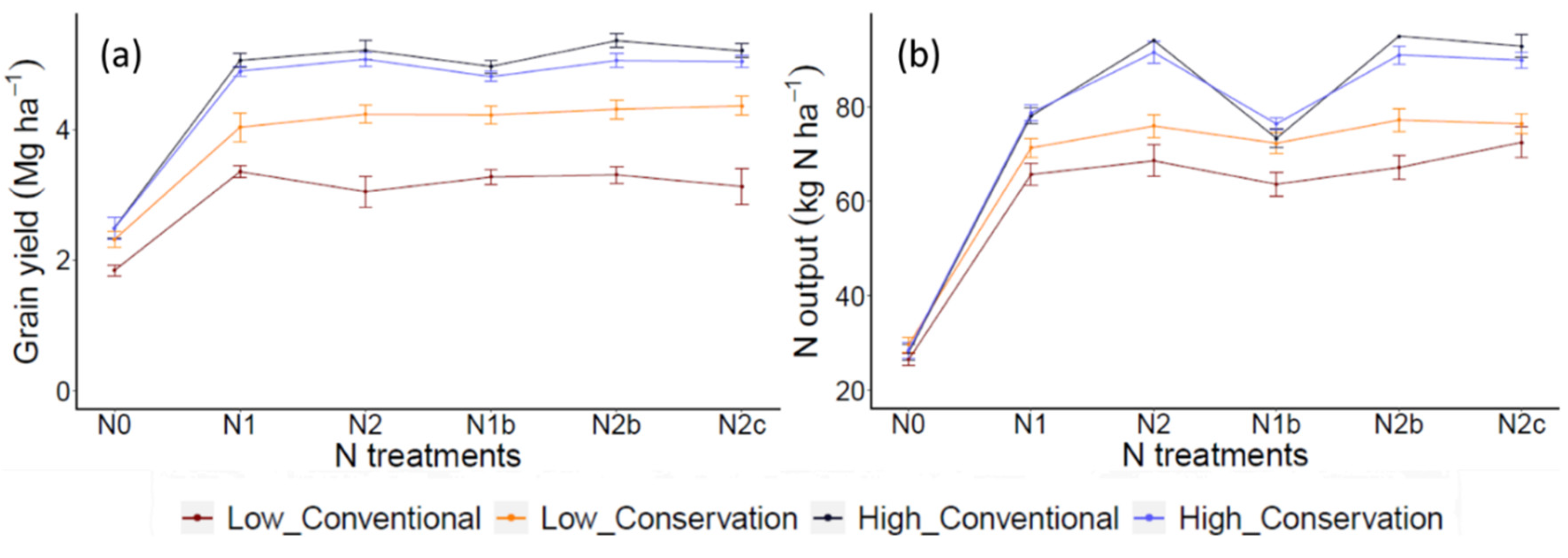
3.1.1. Grain Yield and Biomass

Conservation tillage increased GY and biomass compared to conventional tillage with two post-plant irrigations, whereas with four post-plant irrigations, no differences were found between tillage treatments, suggesting that conservation tillage increased water availability, particularly during the grain filling period (Figure 3a; Table S5; Figure S9). This effect was clearly observed in three out of the four years, 2017 being the exception with small GY differences between tillage treatments and no differences for biomass.
In general, higher irrigation led to higher GY and biomass, enhancing crop N response (Figure 3a). Unfertilized wheat (N0) and fertilized treatments (either N1 or N2) were differentiated with low irrigation, but only with higher irrigation did differences between N doses (N2 > N1) become significant for some of the years. Therefore, the results indicate that the interaction between N and the water effect was relevant.

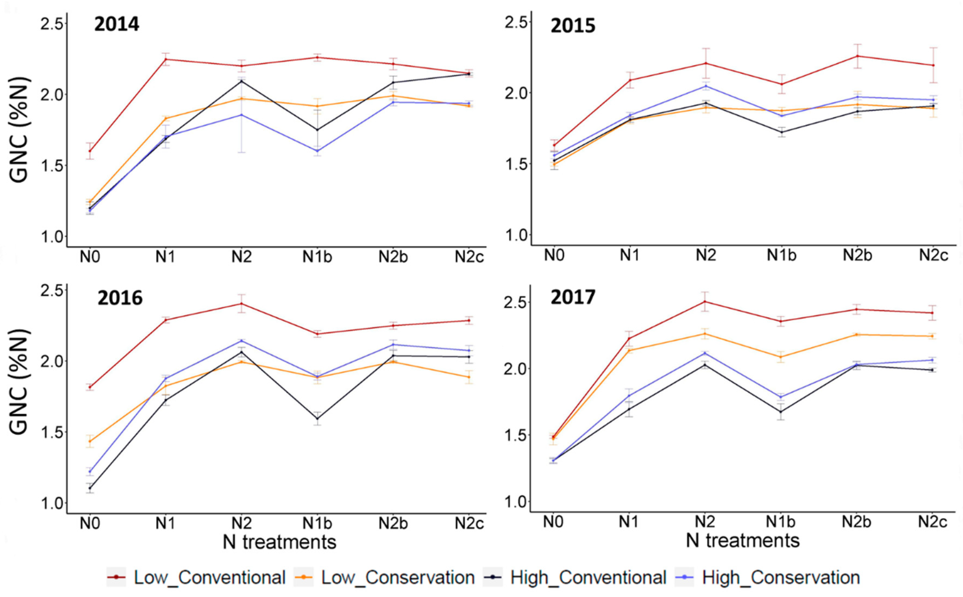
3.1.2. Grain N Concentration and N Output

A strong interaction effect on GNC was observed among all factors and years (Table S5; Figure 4). Lower irrigation tended to produce a higher GNC, but the significance of this increase varied from year to year, depending on the N treatment (Figure 4). In addition, N fertilization increased GNC compared to unfertilized wheat (N0). In contrast, splitting N fertilizer application did not have a significant effect. With low irrigation, differences in GNC between N1 and N2 only were present in 2017; whereas with higher irrigation, increasing the N dose (N2 vs. N1) enhanced GNC every year.
Conventional tillage increased GNC compared to conservation tillage when the irrigation dose was low (mainly when wheat was fertilized), whereas with higher irrigation no differences were found between tillage treatments. Similar to GY and biomass, the interaction of GNC with year was due to small differences in 2017.
Higher irrigation led to a greater N output, and no differences were observed between tillage treatments, whereas with low irrigation, conservation tillage led to higher values compared to conventional tillage (Figure 3b). In general, almost all the years studied showed differences among the three N rates, which was more evident in treatments that received a higher irrigation level.
Overall, the large variability in the effect of the management factors on the variables studied and the relevance of the interaction effects suggests that there is an opportunity for remote sensing to be used as a tool for guiding N fertilizer recommendation in season.

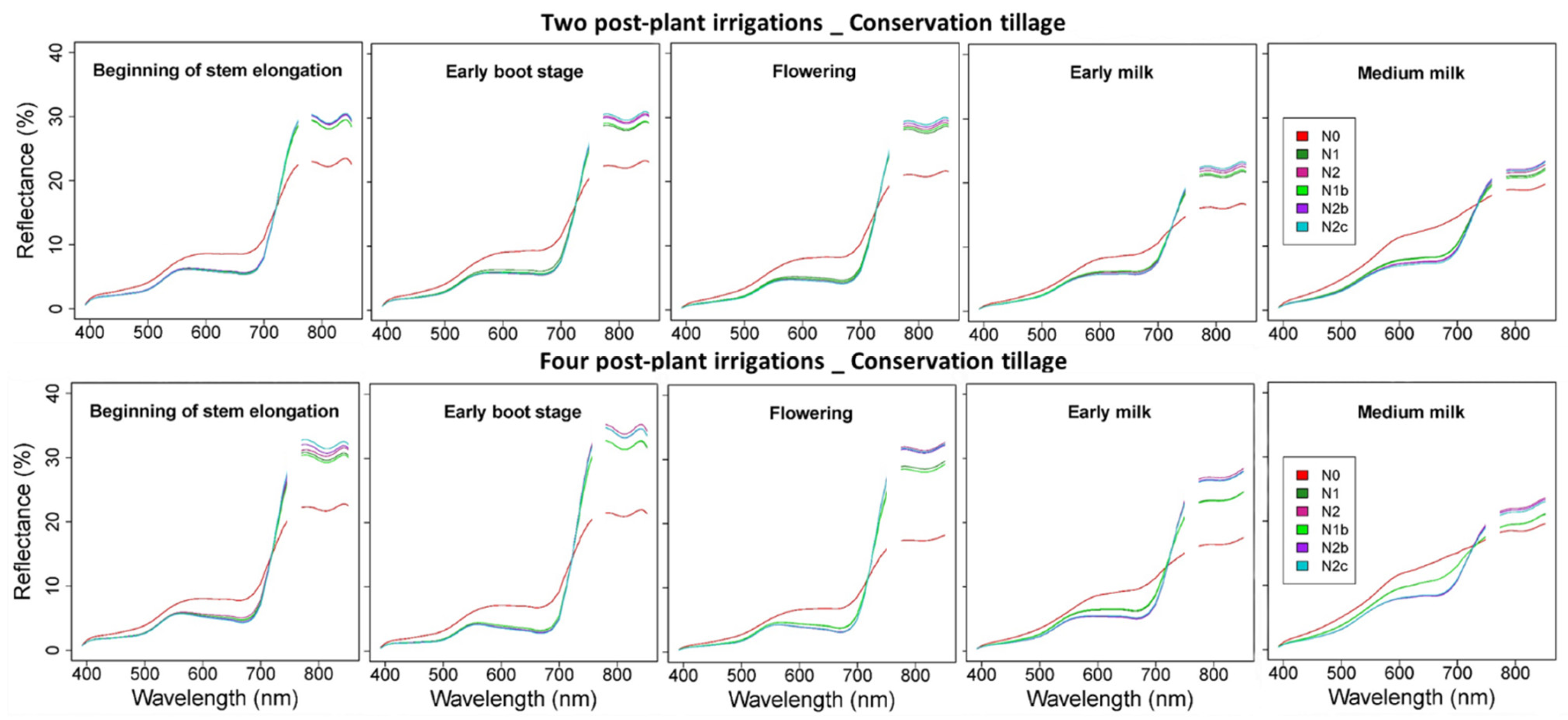
3.2. Spectral Signatures of the Treatments

Differences in reflectance between fertilized and unfertilized treatments were observed from the beginning of stem elongation, and by the medium milk GS these differences declined, particularly for treatments with lower irrigation (Figure 5; Figure S10). In general, fertilized treatments showed lower reflectance in the visible region and higher reflectance in the NIR than the unfertilized wheat (N0), leading to a steeper slope in the red-edge. The greatest difference between treatments was observed in the NIR (>750 nm), where higher reflectance was attained (Figure 5; Figure S10). The NIR reflectance for N0 was always lower than for the fertilized treatments and the maximum reflectance was observed from stem elongation to flowering, with differences between spectral signatures greater at the early milk GS.
The same pattern was repeated every year: reflectance for the fertilized treatments was greater for high irrigated treatments than for those with lower irrigation. Conservation tillage led to a higher reflectance compared to conventional tillage, probably because of increased water availability but to a lesser degree than irrigation. Particularly, in 2014 and 2017 the treatments with low irrigation and conservation tillage resulted in similar reflectance to high irrigated conventional tillage. For N0, differences between irrigation and tillage treatments were much lower. Regarding N fractionation, the effect in reflectance was less clear: only slight differences were observed between treatments at certain GSs, and the signatures of the same N dose followed a similar pattern. Overall, these spectral observations were consistent with the agronomic data at harvest, particularly with yield and N output, which encouraged us to undertake a detailed exploratory analysis.

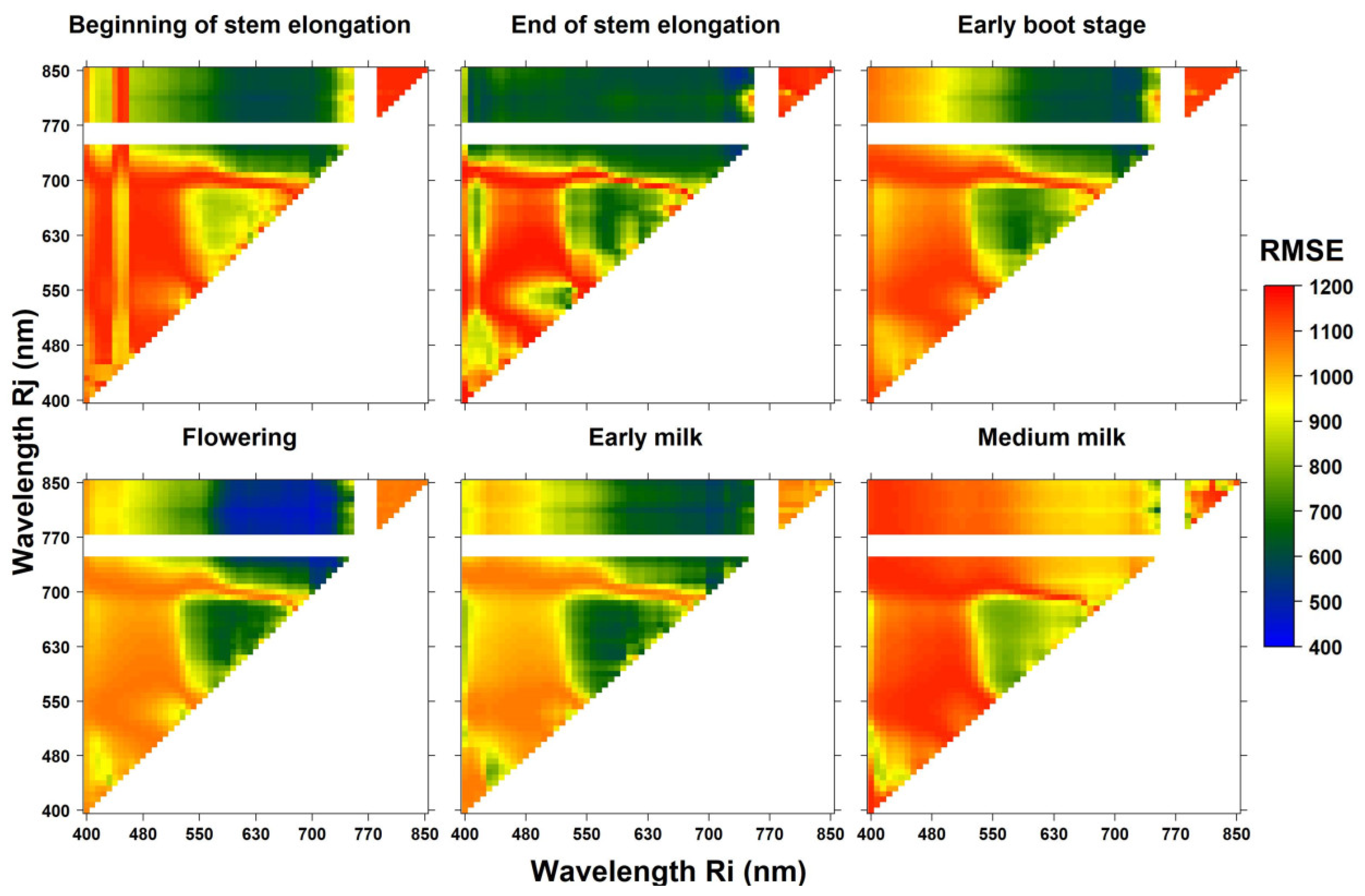
3.3. Spectral Exploratory Analysis Using Narrow-Band Combinations

3.3.1. Grain Yield and Biomass

Differences throughout the various GSs were observed for GY, which obtained the highest relationship between the NDSI and the variable between the beginning of stem elongation towards early milk, with the peak at flowering (Figure 6; Figure S11). The best wavelength combination was found between the broad parts of the NIR (Rj, 750–850 nm, except 751, 759, 766, and 773 nm, which were previously removed) combined with parts of the visible (Ri, 398–707 nm) and red-edge regions (Ri, 720–740 nm). These results were followed by band combinations in the visible region (Rj, 574–665 nm) with the green regions (Ri, 530–619 nm) and other peaks in the blue regions (Rj and Ri, 398–486 nm), which were present in the early growth stages (Figure 6; Figure S11).
At flowering, the best relationships were observed, obtaining a RMSE as low as 400–500 kg ha−1 in the combinations of NIR with the visible regions, and between 600 and 700 kg ha−1 if only bands from the visible region were combined. At earlier GSs, the same regions of contour maps showed lower RMSE values with GY (RMSE > 600 kg ha−1; Figure 6). The R2 followed a similar trend as the RMSE, reaching values > 0.8 for the combinations of NIR and visible bands at flowering and 0.7 at stem elongation (Figure S11). Similar results were found for biomass in the same growth stages, reaching the best combinations at flowering with RMSE between 800 and 1400 kg ha−1 and R2 ranging from 0.4 to 0.8 (Figures S12 and S13).

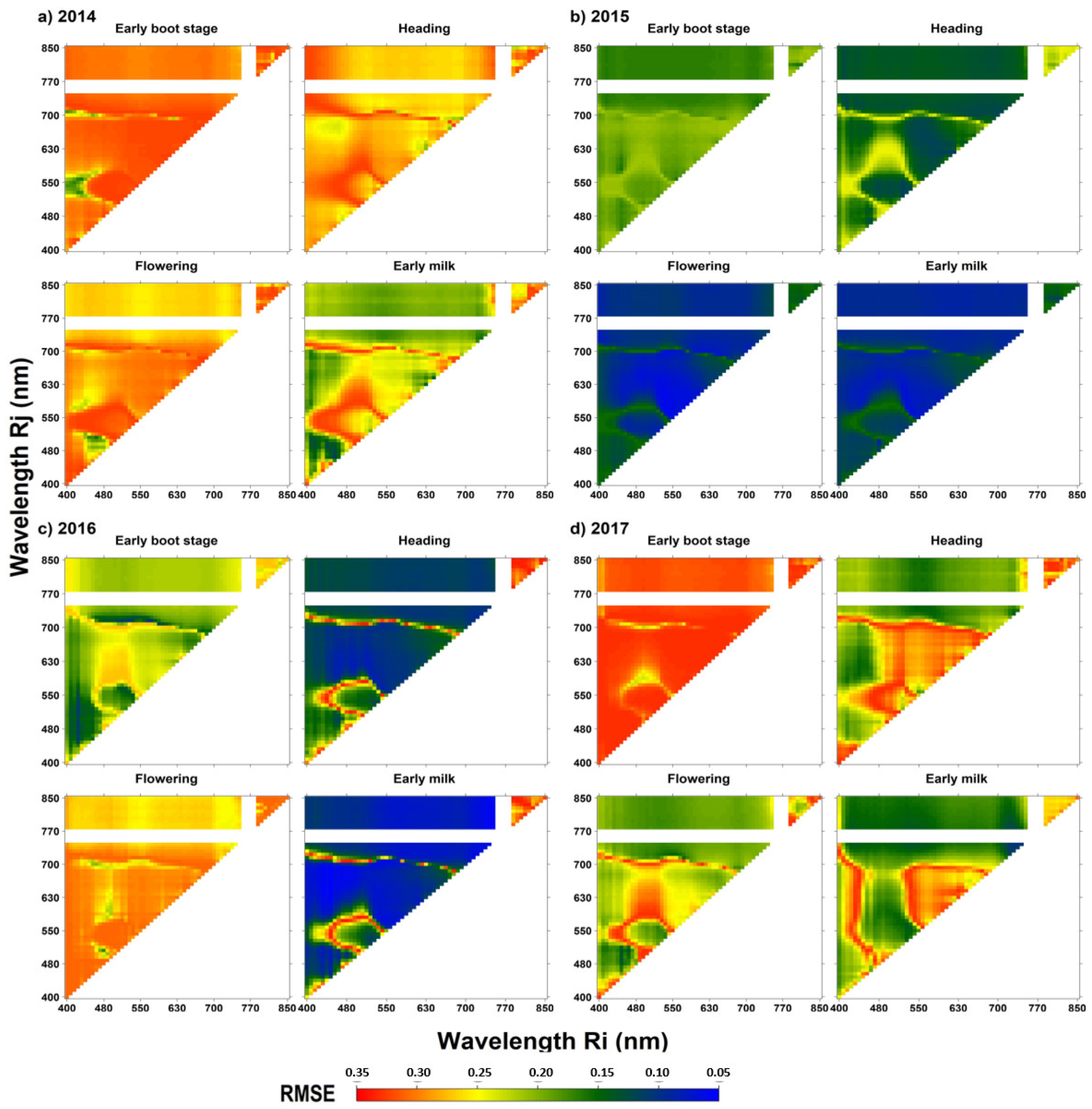
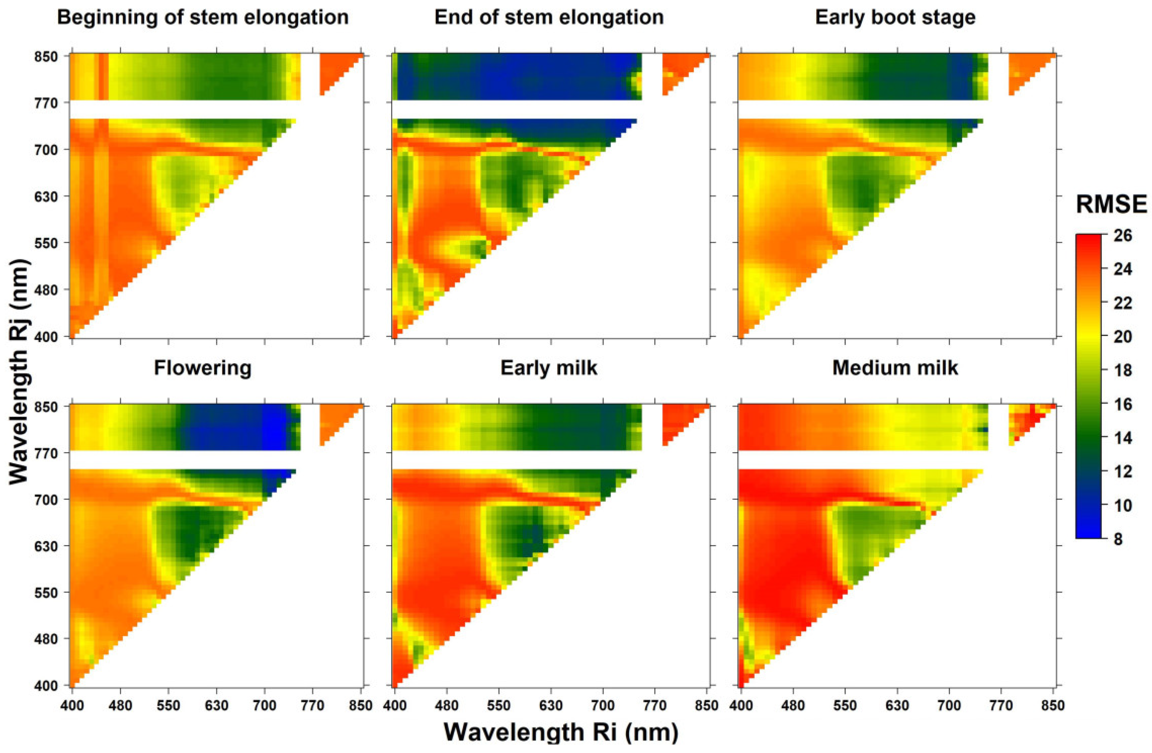
3.3.2. Grain N Concentration and N Output

The spectral exploratory analysis was conducted for all individual years for GNC due to the significant year interaction observed in the agronomic results (Table S5). Accordingly, contour maps showed differences among years in both GS performance and best wavelength combination (Figure 7 and Figure S14). Generally, the relationship between GNC and the spectral bands improved from booting to early milk, but in 2016 it was better at heading than at flowering. A common pattern to all years was that early milk was the best GS to assess GNC, reflecting a RMSE as low as 0.05%N in 2015 and 2016, and 0.15%N in 2014 and 2017. From the medium milk stage on, the relationship declined sharply in all years. At booting, a relevant GS for fertilizer recommendation, some spectral regions presenting a significant relationship with GNC had already appeared and were highly significant in later GSs.
The predominantly high wavelength combinations had some common distribution patterns among years, emphasizing NIR and red-edge regions (707–850 nm) on Rj combined with a broad range on Ri (398–740 nm). Narrower wavelength combinations in the visible range performed well, such as 398–530 nm on Rj and 398–486 nm on Ri as well as 574–665 nm on Rj combined with 398–486 nm and 530–619 nm on Ri. In addition, the area around the green region (Rj and Ri 530 nm) was highlighted in the contour maps of most of the GSs (Figure 7).
The relationship of N output with wavelength combinations was similar to GY and biomass, with the difference that the NIR (Rj, 750–850 nm) together with the red-edge region (Ri, 720–740 nm) showed a low RMSE (Figure 8). These results indicate the excellent predictive ability of these wavelength regions for N output, mainly between the end of stem elongation and flowering, obtaining a RMSE ranging from 8 to 12 kg N ha−1 and R2 between 0.6 and 0.8 (Figure 8; Figure S15).

3.4. Spectral Indices and Assessment of Crop Variables

3.4.1. Grain Yield and Biomass

The structural indices (NDVI and reformed difference vegetation index (RDVI)) were highly correlated with GY and biomass in all GSs (Table 2). The best statistical performance of these indices was achieved at flowering, when the R2 > 0.70 and RMSE < 596 and 988 kg ha−1 for GY and biomass, respectively. At the early milk stage, the correlations were slightly lower than at flowering but still high in both agronomic variables. The highest correlations occurred at flowering (Table 2). The chlorophyll indices normalized difference red-edge (NDRE) and red-edge optical reflectance (R750/R710), and the canopy index CCC also showed a significant correlation with GY and biomass; in particular, at flowering R2 > 0.65 in all cases, and the RMSE < 664 kg ha−1 for GY and biomass. Nevertheless, the other structural (normalized green (NG)), chlorophyll (double peak canopy nitrogen index (DCNI), modified chlorophyll absorption ratio index (MCARI)), and canopy (canopy chlorophyll content index (CCCI), and nitrogen planar domain index (NDPI)) indices did not present a good relationship with these agronomic variables. Therefore, VIs that combined NIR and the visible bands were the best GY and biomass predictors. All VIs showed worse predictive ability during the period before flowering.

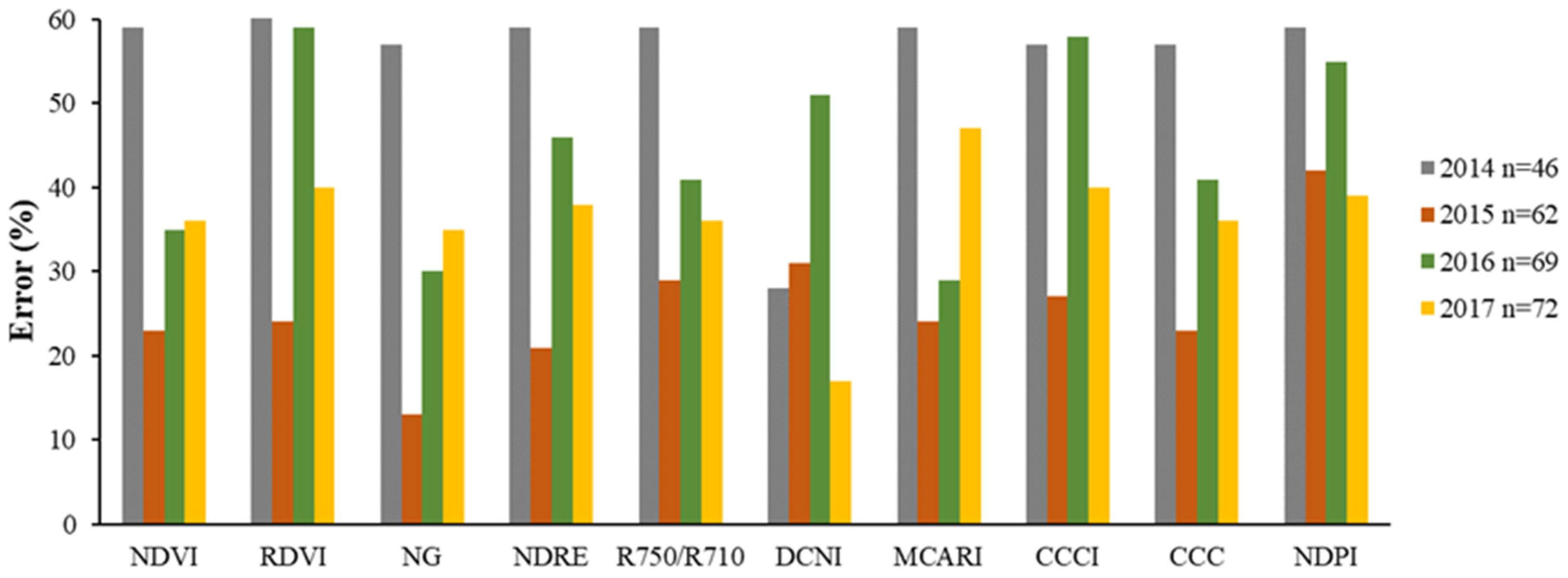
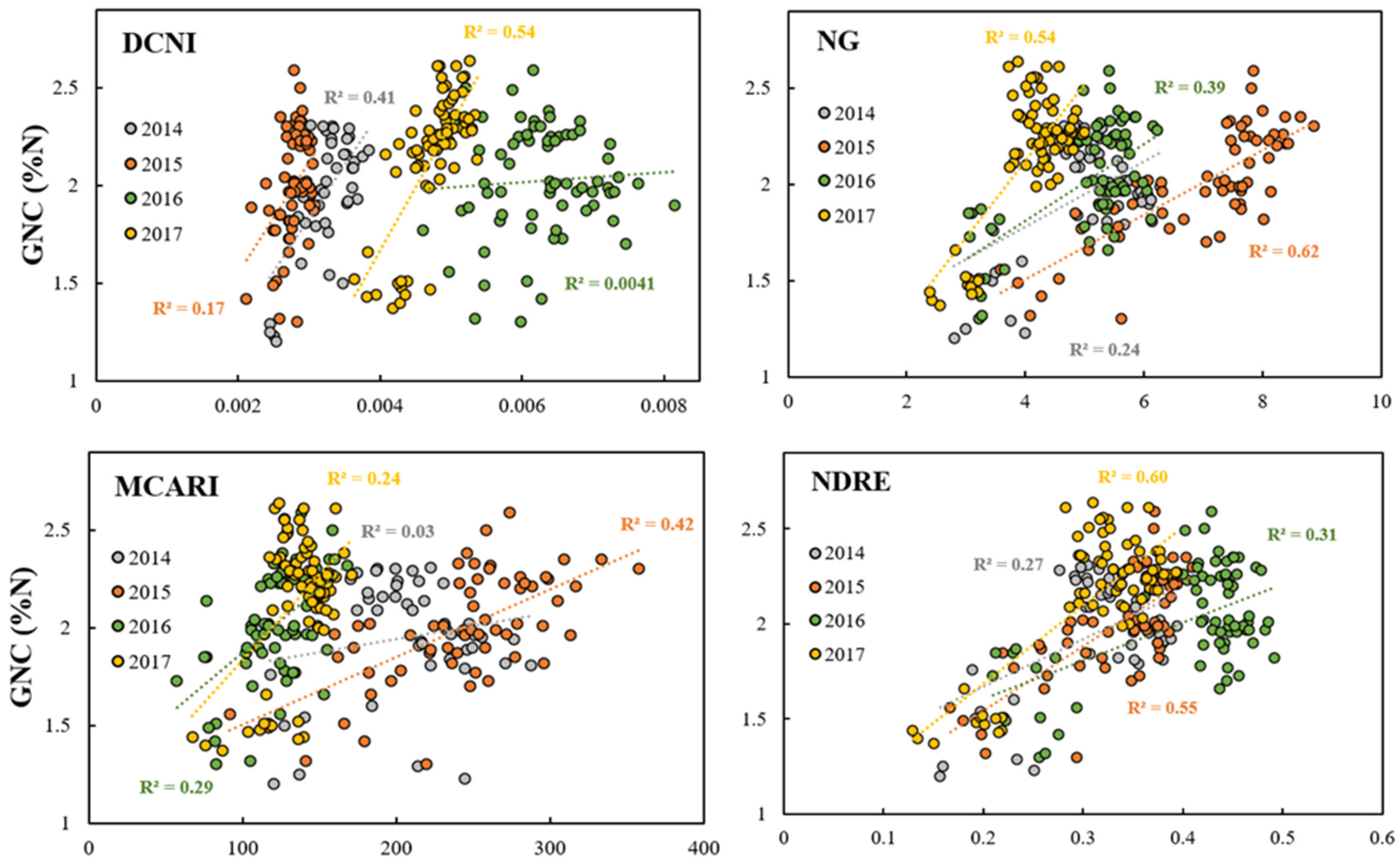
3.4.2. Grain N Concentration and N Output

The overall VI performance for GNC was the worst among the agronomic variables evaluated, with great variability between years and growth stages (Table 3), agreeing with the results observed in the contour maps (Figure 7).
At booting, only the DCNI and CCCI showed R2 > 0.45 in 2014 and 2017, whereas the rest of the VIs showed low R2 in all years. In addition, the R2 for the DCNI and CCCI was very low and the relationship with GNC not significant in 2015 and 2016. At heading, the relationship between GNC and the VIs tended to improve, performing better on the structural indices NDVI, RDVI, and NG, the chlorophyll indices NDRE and R750/R710, and the canopy indices CCC and NDPI in 2016 (R2 > 0.80, RMSE < 0.15%N), and NG in 2017 (R2 = 0.68, RMSE = 0.2%N). At flowering, the R2 of the relationship between all the indices and GNC was < 0.60 for all years. At the early milk stage, the most outstanding indices were the DCNI, in 2014 and 2015; the structural indices (NDVI, RDVI, and NG), the chlorophyll indices NDRE and R750/R710, together with the canopy chlorophyll indices (CCC, CCCI, and NDPI) in 2016; and the chlorophyll indices (NDRE and R750/R710) together with the structural indices (NDVI, RDVI, and NG) and canopy indices (CCC and NDPI) in 2017 (Table 3).
The relationship between the spectral indices and N output was better for the images acquired at the flowering and early milk stages than at the beginning of stem elongation (Table 4). The chlorophyll indices NDRE and R750/R710, both the structural (NDVI and RDVI) and the canopy index CCC showed significant linear correlations with N output in all growth stages, obtaining R2 > 0.7 and RMSE < 12 kg N ha−1 at flowering and early milk (Table 4). The best performance was obtained with NDRE, which achieved an R2 of 0.84 and RMSE of 9 kg N ha−1 at flowering. Similar to GY and biomass, the DCNI, MCARI, NG, CCCI, and NDPI indices provided lower correlations than the previous indices for N output. According to these results, the spectral indices calculated from red-edge bands and NIR and red band combinations were more consistent in assessing N output.

3.5. Application to N Fertilizer Recommendation for Increasing GNC

For three out of the four years studied, the chlorophyll indices showed lower errors than the rest of the indices in identifying plots that were responsive and nonresponsive to a topdressing N fertilizer application within the low irrigated treatments (Figure 9). The lowest error was achieved using the DCNI in 2014 and 2017 (28% and 17%, respectively) and using the MCARI in 2016 (29%). In 2015, the lowest error was obtained using NG (13%) followed by NDRE (21%).
These results agree with the linear correlations between the indices and GNC (Figure 10). The VIs that incorporated information from the red-edge bands (DCNI, MCARI, and NDRE) and NIR-green combinations (NG) obtained higher R2 in the years in which they are better able to discriminate GNC responsive and nonresponsive sites (Figure 9). However, although the chlorophyll indices showed potential for N fertilization at booting, a great variability between VIs and years was observed and there was not a single index that performed well every year.

4. Discussion

4.1. What Are the Best Indices for Estimating GY, Biomass, GNC, and N Output

This study confirms the great potential that remote sensing has for GY and biomass assessment in spring wheat. The highest assessment potential came from band combinations in the NIR and the red-edge as well as the NIR and visible region; therefore, the so-called structural indices such as the NDVI and RDVI were among the best predictors of GY. The high assessment potential for wheat GY of band combinations from the NIR and red-edge regions was reported in previous studies that discussed the advantage of using narrow bands that capture the abrupt changes in the red-edge region [10,11,63,64]. In the current study, the visible and NIR band combinations provided a high assessment ability. This is in agreement with some of the literature [17,22,25,65] but not with other studies that reported a low relationship in wheat and other crops [19,59,66,67,68,69]. These low relationships were attributed to differences in canopy cover and soil background. Indices that estimated chlorophyll activity at the canopy level were able to provide a better relationship with crop status and yield in Australia, Italy, and the US [19,57,69]. In the current study, a uniform ground cover was observed in all plots, probably because they were all irrigated. This may be part of the reason for the better performance of structural and canopy indices as predictors of GY, which were consistent during the four years. It is remarkable that despite the significant impact of irrigation level and tillage practices on wheat productivity, GY, and biomass were accurately predicted over the four years. The other reason may be the combination of the genotype and planting method employed in this study. CIRNO C2008, the genotype used in this study, is durum wheat, which tends to have upright leaves as opposed to the floppy leaves in bread wheat. Moreover, this genotype is shorter than most durum cultivars, so these two canopy architecture traits limit the ability of the crop to cover the ground rapidly. In addition, the planting method utilized—two rows 25 cm apart on top of an 80-cm bed leaving a 55-cm gap between rows in different beds—also, limited the ability of the canopy to fully cover the ground and maximize yield [70]. Therefore, the use of a genotype sensitive to wide row spacing reduced the possibility of the VIs reaching saturation.
The GNC response to the N fertilization rate or splitting was more erratic among years than GY. Grain N concentration responded to the highest N rate in various years and treatment combination, whereas splitting fertilization did so only occasionally. When the response occurred, it was usually coupled to a higher reflectance value, particularly in NIR. The higher assessment potential came from band combinations in NIR and red-edge at the early milk GS. Some of the years, band combinations from the visible region showed good performance (i.e., 2015, and 2016), but this was not consistent in all four years. This is in agreement with results from Rodrigues et al. [23], who obtained the best relationship between grain protein concentration and band combinations from the red-edge and green region, even if the relationship in the field study was very weak (R2 ≤ 0.21). Prey and Schmidhalter [11] also emphasized the potential for the red-edge to assess grain N concentration, although lack of consistency between years was mentioned in their study. This variability across studies and years may be associated with the great variation in grain N concentration among genotypes and environmental conditions [30].
A novelty of this study is that it shows the potential of remote sensing for assessing N output, calculated as the product of GY and GNC. Band combinations in NIR and red-edge provided the highest assessment potential; therefore, indices such as NDRE that account for pigment content were among the best predictors. Estimation of N output is useful in forage crops and also an important indicator of N productivity of the agro-ecosystem and key to calculating NUE [40,71].

4.2. When Is the Best Growth Stage for Assessing GY, Biomass, GNC, and N Output

The best GS for yield assessment was between the end of flowering and early milk stages. The RMSE that resulted when using reflectance indices from flowering to grain development was as low as 400 kg ha−1 during a four-year period, with the mean of the highest yield obtained at 5250 kg ha−1. At the late milk stage, the error increased, probably due to the decrease in reflectance associated with crop senescence. Increasing R2 values between reflectance indices and wheat GY from early growth stages to flowering or grain filling is a common trend reported in the literature. However, differences during the best GSs were mainly genotype-dependent [66]. When using visible/NIR combinations, the RMSE was higher at flowering than at grain filling, probably due to changes in growth and morphological interferences associated with anther exposure [22,72]. However, the red-edge/NIR combination was not affected by these interferences and the lowest RMSE with GY was observed at flowering. These results are in agreement with observations from Prey and Schmidhalter [11], who recommended avoiding anthesis for grain yield assessment, particularly when using broad bands that cannot capture red-edge changes.
For GNC assessment, the best GS was early milk stage. The RMSE of the prediction depended on the year, whereas in 2015 and 2016 the RMSE was as low as 0.05%N, and in 2014 and 2017 was between 0.15 and 0.2%N. Given that the quality criteria for durum wheat ranges between 2.2 and 2.3%N depending on the country, a RMSE > 0.2%N implies high uncertainty in the prediction. Grain N concentration depends on the N accumulated in the biomass at flowering, but it is also strongly influenced by temperature and water access during grain filling [73,74]. High temperature and water stress during grain filling enhance GNC [75,76]. Consequently, the year effect becomes very important even for the same wheat genotype, and even if increases in GNC are often associated with a GY reduction due to a dilution effect, this relationship could be the reverse or not significant [58,77]. In the present study, differences in water availability during grain filling came from both irrigation and the tillage effect, highlighting the need to evaluate if information from crop water status could improve the assessment of GNC. This is precisely one of our current lines of research where we are evaluating crop water status using soil measurements as well as canopy temperature measured with infrared cameras. The aim of this research is to establish a better assessment of GNC by adding water related proxies to our analysis.
Finally, the best growth stages for N output prediction were stem elongation, booting, and flowering. When using reflectance indices from flowering to grain development, the RMSE was as low as 8–9 kg N ha−1 during a four-year period, accounting for about 10% of the N output. At early milk, the combination of NIR and red bands resulted in an error of 11–12 kg N ha−1, which increased drastically at the late milk stage. Indices were able to capture the N output response to the highest N dose observed in high irrigated treatments, which was not observed in the treatments with low irrigation.

4.3. Use of Spectral Information to Guide Fertilizer Recommendation

The application of in-season measurements of crop reflectance for developing strategies that enable site-specific N fertilizer recommendation has been one of the most investigated topics to enhance N use efficiency in the last decades [14,78]. Algorithms based on spectral sensor readings have been developed and used in precision agriculture to recommend management zones with variable fertilizer application rate [17,79]. Fertilizer recommendation made using these algorithms rely on the in-season prediction of (i) GY potential, and (ii) crop response to N application. The spectral exploratory analysis conducted in our experiment proved the predictive accuracy in GY and showed limitations for prediction of GNC. Furthermore, the information obtained by the complete two by two combination of wavelengths presents the possibility to support technological progress, allowing better decision-making in the development of new sensors and indices for specific goals (i.e., improving grain quality).
With the data available in this study, we were able to evaluate the potential of remote sensing to identify plots in which GNC respond to N application from nonresponsive plots. Identification of GNC responsive plots at booting is crucial because this information would allow applying fertilizer only to responsive sites. When the objective is enhancing GNC in spring wheat, common strategies are increasing soil N availability by late applications (i.e., booting or heading) of either fertilizer to the soil or foliar N applications that can be readily taken up [80,81]. These strategies are particularly suitable for remote sensing detection of crop nutritional status given that canopies are already fully developed. Identification of responsive sites provides the opportunity for the use of variable-rate application machines that will deliver the right N rate spatially throughout the field. In this study, the lowest error in the identification of plots prone to respond to an increase in N application after booting was achieved with chlorophyll indices based on the combination of NIR/red-edge bands (DCNI, NDRE, and MCARI), emphasizing the role of the narrow-band type of sensors in precision agriculture. However, it is interesting to note that the simple ratio of NIR and green bands (NG) provided the best relationship with GNC in 2015 and performed better than the other structural indices in the rest of the years. This is in agreement with Daughtry et al. [52], who reported a good response of the NIR/green ratio with chlorophyll content in maize, and showed the potential of some structural indices, easily adaptable to relatively broad bands, to estimate GNC. Nevertheless, there was not a single index that provided reliable recommendations every year and the error in identifying responsive from nonresponsive sites was >20% in two of the years studied. Therefore, there is still a need to clarify if information from other stress factors could reduce the error consistently to levels acceptable for decision making. Furthermore, emerging machine learning techniques based on ensemble methods (i.e., random forest, and neuronal networks) that already showed potential in obtaining robust outcomes in agri-environmental studies [82,83] could be used to combine the information form other stress factors allowing better decision-making in precision agriculture.

5. Conclusions

Indices based on the combination of bands from NIR and visible regions (NDVI, and RDVI) and from NIR and red-edge regions (NDRE) provided the higher assessment potential of spring wheat grain yield. Grain N concentration and N output were better estimated by indices that combined bands in the NIR and the red-edge. The best growth stage for the yield assessment took place from the end of flowering to early milk, when the RMSE was below 700 kg ha−1 of the yield during a four-year period. For GNC the best growth stage was early milk across treatments. Grain N concentration response to N treatment varied with years and depended on the irrigation level and tillage. The response was usually detected by changes in reflectance, but reliable assessment of GNC in wheat by remote sensing remains challenging. Nitrogen output was better assessed at booting-heading, when the RMSE in the assessment was as low as 8–9 kg N ha−1 during a four-year period (≈10% of the average N output). Overall, broad bands from multispectral sensors could be used to assess wheat yield, but reliable assessment of grain N concentration and N output were obtained using narrow bands from a hyperspectral sensor.
The use of remote sensing to guide fertilizer recommendations for increasing GNC based on structural and canopy-related indices at booting resulted in an error greater than 20% in the identification of responsive sites. Identification of GNC responsive sites was better estimated by chlorophyll indices that combine NIR and narrow red-edge bands such as the DCNI, NDRE, and MCARI, but the simple ratio of NIR and green bands (NG) was also promising. However, the error in identifying GNC responsive sites should be reduced before the application of this approach to precision agriculture.

Supplementary Materials

The following are available online at https://www.mdpi.com/article/10.3390/rs13071373/s1, Figure S1: Monthly rainfall (blue bars), average maximum temperatures (continuous lines) and average minimum temperatures (dashed lines) during the experiment in the Yaqui Valley (Sonora, Mexico). Table S1: Critical dates (sowing, harvest, fertilization, irrigation) for the field experiment and for the two irrigation blocks during the 4 experimental years. Table S2: Selected dates of image acquisition and the corresponding wheat growth stage (GS) of the two irrigation blocks during the 4 experimental years. Names of the relevant GSs for the analysis are in parentheses in addition to the decimal code. Table S3: Reflectance used to calculate the airborne indices and the exact bands of the hyperspectral image from which the reflectance was extracted. Table S4: Airborne hyperspectral indices calculated in this study. Figure S6: Correlograms of the vegetation indices calculated as in Table S4. The value inside each square of the grid is the coefficient of correlation (r value) at P ≤ 0.01 for different years: (a) 2014, (b) 2015, (c) 2016 and (d) 2017. Figure S7: Linear and exponential relationship between spectral indices (NDVI, R750/R710, and CCC) and crop variables (yield, biomass and N output) at flowering. The X-axis represents the spectral index values and the Y-axis the crop variable values. Dotted lines are the adjusted linear (black) and exponential (red) model and R2 its coefficient of determination. Table S5: Results (P-value) of the analysis of variance between irrigation (irr), tillage (till), N treatment (nlevel) and year, and their combined interactions on the wheat grain yield, total above-ground biomass, grain N concentration (GNC) and N output at harvest. Figure S9: Biomass for combined tillage and irrigation factors, for each N treatment, over the 4 years. Small bars indicate SE. Figure S10: Spectral reflectance (%) from 400 nm to 850 nm, for the different N treatments (N0, N1, N1b, N2, N2b, N2c) with conventional tillage, either with two post-plant irrigations (top row), or with four post-plant irrigations (bottom row), at five growth stages, in 2014. Figure S11: Contour maps of the coefficient of determination (R2) between the NDSI (Ri, Rj) and grain yield using the complete combinations of two wavelengths at i and j nm within the range 400–850 nm. At each growth stage, data from the different years were merged to build the figure (4 years for all the GSs and 2 for the end of stem elongation and early milk stages). Figure S12: Contour maps of the root mean square error (RMSE, kg ha−1) between the NDSI (Ri, Rj) and biomass using the complete combinations of two wavelengths at i and j nm within the range 400–850 nm. At each growth stage, data from the different years were merged to build the figure (4 years for all the GSs and 2 for the end of stem elongation and medium milk stages). Figure S13: Contour maps of the coefficient of determination (R2) between the NDSI (Ri, Rj) and biomass using the complete combinations of two wavelengths at i and j nm within the range 400–850 nm. At each growth stage, data from the different years were merged to build the figure (4 years for all the GSs and 2 for the end of stem elongation and medium milk). Figure S14: Contour maps of the coefficient of determination (R2) between the NDSI (Ri, Rj) and Grain N concentration using the complete combinations of two wavelengths at i and j nm within the range 400–850 nm, at different growth stages for different years: (a) 2014, (b) 2015, (c) 2016, and (d) 2017. Figure S15: Contour maps of the coefficient of determination (R2) between the NDSI (Ri, Rj) and N output using the complete combinations of two wavelengths at i and j nm within the range 400–850 nm. At each growth stage, data from the different years were merged to build the figure (4 years for all the GSs and 2 for the end of stem elongation and medium milk stages).

Author Contributions

Conceptualization, M.D.R.-S., J.I.O.-M. and M.Q.; methodology, J.I.O.-M., L.G.-P. and M.Q.; formal analysis, M.A.-A. and A.A.R.; investigation, M.D.R.-S., J.I.O.-M., M.A.-A., L.G.-P., F.A.R.J., A.A.R. and M.Q.; resources, J.I.O.-M. and M.Q.; writing—original draft preparation, M.D.R.-S., M.A.-A. and M.Q.; writing—review and editing, M.D.R.-S., J.I.O.-M., M.A.-A., F.A.R.J., L.G.-P., A.A.R. and M.Q..; visualization, M.D.R.-S., M.A.-A., L.G.-P., F.A.R.J. and A.A.R.; supervision, J.I.O.-M. and M.Q.; funding acquisition, J.I.O.-M. and M.Q. All authors have read and agreed to the published version of the manuscript.

Funding

This research was supported by the Consultative Group on International Agricultural Research (CGIAR) research program on wheat agri-food systems (CRP WHEAT—www.wheat.org, accessed on 5 March 2021), the Comunidad de Madrid (AGRISOST-CM S2018/BAA-4330 project), the European Structural Funds 2014–2020 and the UK Space Agency’s International Partnership Program (IPP) funded from the Department for Business, Energy and Industrial Strategy’s (BEIS) Global Challenges Research Fund (GCRF). The funders had no role in the study design, data collection and analysis, decision to publish, or preparation of the manuscript. The views expressed here are those of the authors and do not necessarily reflect the views of the funder or associated institutions. The Spanish Ministry of Education provided financial support to María D. Raya-Sereno (FPU17/01251). The usual disclaimer applies.

Institutional Review Board Statement

Not applicable.

Informed Consent Statement

Not applicable.

Data Availability Statement

The data presented in this study are available on request from the corresponding author.

Acknowledgments

We would also like to thank Maria Elena Cardenas and Delia Gallegos for data management and Jorge Miranda, Alan Medrano and Indalecio Galvez for field support activities.

Conflicts of Interest

The authors declare no conflict of interest.

References

  1. Matson, P.A.; Naylor, R.; Ortiz-Monasterio, I. Integration of environmental, agronomic, and economic aspects of fertilizer management. Science 1998, 280, 112–115. [Google Scholar] [CrossRef] [Green Version]
  2. Arregui, L.M.; Quemada, M. Strategies to improve nitrogen-use efficiency in winter cereal crops under rainfed Mediterranean conditions. Agron. J. 2008, 100, 277–284. [Google Scholar] [CrossRef]
  3. Food and Agriculture Organization of the United Nations. World Fertilizer Trends and Outlook to 2019; Food and Agriculture Organization of the United Nations: Rome, Italy, 2016. [Google Scholar]
  4. Galloway, J.N.; Townsend, A.R.; Erisman, J.W.; Bekunda, M.; Cai, Z.; Freney, J.R.; Martinelli, L.A.; Seitzinger, S.P.; Sutton, M.A. Transformation of the nitrogen cycle: Recent trends, questions, and potential solutions. Science 2008, 320, 889–892. [Google Scholar] [CrossRef] [PubMed] [Green Version]
  5. Harrison, J.; Matson, P. Patterns and controls of nitrous oxide emissions from drainage waters of the Yaqui Valley, Sonora, Mexico. Glob. Biogeochem. Cycles 2003, 17, 1080. [Google Scholar] [CrossRef]
  6. Beman, J.M.; Arrigo, K.R.; Matson, P.A. Agricultural runoff fuels large phytoplankton blooms in vulnerable areas of the ocean. Nature 2005, 434, 211–214. [Google Scholar] [CrossRef] [PubMed]
  7. Colaço, A.F.; Bramley, R.G.V. Site–Year Characteristics Have a Critical Impact on Crop Sensor Calibrations for Nitrogen Recommendations. Agron. J. 2019, 111, 2047–2059. [Google Scholar] [CrossRef]
  8. Hatfield, J.L.; Gitelson, A.A.; Schepers, J.S.; Walthall, C.L. Application of spectral remote sensing for agronomic decisions. Agron. J. 2008, 100, 117–131. [Google Scholar] [CrossRef] [Green Version]
  9. Haboudane, D.; Miller, J.R.; Tremblay, N.; Zarco-Tejada, P.J.; Dextraze, L. Integrated narrow-band vegetation indices for prediction of crop chlorophyll content for application to precision agriculture. Remote Sens. Environ. 2002, 81, 416–426. [Google Scholar] [CrossRef]
  10. Hansen, P.M.; Schjoerring, J.K. Reflectance measurement of canopy biomass and nitrogen status in wheat crops using normalized difference vegetation indices and partial least squares regression. Remote Sens. Environ. 2003, 86, 542–553. [Google Scholar] [CrossRef]
  11. Prey, L.; Schmidhalter, U. Simulation of satellite reflectance data using high-frequency ground based hyperspectral canopy measurements for in-season estimation of grain yield and grain nitrogen status in winter wheat. ISPRS J. Photogramm. Remote Sens. 2019, 149, 176–187. [Google Scholar] [CrossRef]
  12. Gabriel, J.L.; Zarco-Tejada, P.J.; López-Herrera, P.J.; Pérez-Martín, E.; Alonso-Ayuso, M.; Quemada, M. Airborne and ground level sensors for monitoring nitrogen status in a maize crop. Biosyst. Eng. 2017, 160, 124–133. [Google Scholar] [CrossRef]
  13. Peñuelas, J.; Filella, I.; Biel, C.; Serrano, L.; Save, R. The reflectance at the 950–970 nm region as an indicator of plant water status. Int. J. Remote Sens. 1993, 14, 1887–1905. [Google Scholar] [CrossRef]
  14. Fox, R.H.; Walthall, C.L. Crop Monitoring Technologies to Assess Nitrogen Status. In Nitrogen in Agricultural Systems, Agronomy Monograph 49; Schepers, J.S., Raun, W.R., Eds.; ASA, CSSA, SSSA: Madison, WI, USA, 2008; pp. 647–674. [Google Scholar] [CrossRef]
  15. Fischer, R.A.; Howe, G.N.; Ibrahim, Z. Irrigated spring wheat and timing and amount of nitrogen fertilizer. I. Grain yield and protein content. Field Crop. Res. 1993, 33, 37–56. [Google Scholar] [CrossRef]
  16. Ravier, C.; Quemada, M.; Jeuffroy, M.H. Use of a chlorophyll meter to assess nitrogen nutrition index during the growth cycle in winter wheat. Field Crop. Res. 2017, 214, 73–82. [Google Scholar] [CrossRef]
  17. Raun, W.R.; Solie, J.B.; Stone, M.L.; Martin, K.L.; Freeman, K.W.; Mullen, R.W.; Zhang, H.; Schepers, J.S.; Johnson, G.V. Optical sensor-based algorithm for crop nitrogen fertilization. Commun. Soil Sci. Plant Anal. 2005, 36, 2759–2781. [Google Scholar] [CrossRef] [Green Version]
  18. Li, F.; Miao, Y.; Zhang, F.; Cui, Z.; Li, R.; Chen, X.; Zhang, H.; Schroder, J.; Raun, W.R.; Jia, L. In-season optical sensing improves nitrogen-use efficiency for winter wheat. Soil Sci. Soc. Am. J. 2009, 73, 1566–1574. [Google Scholar] [CrossRef] [Green Version]
  19. Fitzgerald, G.; Rodriguez, D.; O’Leary, G. Measuring and predicting canopy nitrogen nutrition in wheat using a spectral index—the canopy chlorophyll content index (CCCI). Field Crop. Res. 2010, 116, 318–324. [Google Scholar] [CrossRef]
  20. Li, F.; Mistele, B.; Hu, Y.; Yue, X.; Yue, S.; Miao, Y.; Chen, X.; Cui, Z.; Meng, Q.; Schmidhalter, U. Remotely estimating aerial N status of phenologically differing winter wheat cultivars grown in contrasting climatic and geographic zones in China and Germany. Field Crop. Res. 2012, 138, 21–32. [Google Scholar] [CrossRef]
  21. Diacono, M.; Rubino, P.; Montemurro, F. Precision nitrogen management of wheat. A review. Agron. Sustain. Dev. 2013, 33, 219–241. [Google Scholar] [CrossRef]
  22. Babar, M.A.; van Ginkel, M.; Klatt, A.R.; Prasad, B.; Reynolds, M.P. The potential of using spectral reflectance indices to estimate yield in wheat grown under reduced irrigation. Euphytica 2006, 150, 155–172. [Google Scholar] [CrossRef]
  23. Rodrigues, F.A.; Blasch, G.; Defourny, P.; Ortiz-Monasterio, J.I.; Schulthess, U.; Zarco-Tejada, P.J.; Taylor, J.A.; Gérard, B. Multi-temporal and spectral analysis of high-resolution hyperspectral airborne imagery for precision agriculture: Assessment of wheat grain yield and grain protein content. Remote Sens. 2018, 10, 930. [Google Scholar] [CrossRef] [PubMed] [Green Version]
  24. Ziadi, N.; Bélanger, G.; Claessens, A.; Lefebvre, L.; Cambouris, A.N.; Tremblay, N.; Nolin, M.C.; Parent, L.É. Determination of a critical nitrogen dilution curve for spring wheat. Agron. J. 2010, 102, 241–250. [Google Scholar] [CrossRef]
  25. Magney, T.S.; Eitel, J.U.H.; Huggins, D.R.; Vierling, L.A. Proximal NDVI derived phenology improves in-season predictions of wheat quantity and quality. Agric. For. Meteorol. 2016, 217, 46–60. [Google Scholar] [CrossRef]
  26. Prey, L.; Schmidhalter, U. Deep Phenotyping of Yield-Related Traits in Wheat. Agronomy 2020, 10, 603. [Google Scholar] [CrossRef] [Green Version]
  27. Stewart, C.M.; McBratney, A.B.; Skerritt, J.H. Site-specific durum wheat quality and its relationship to soil properties in a single field in northern New South Wales. Precis. Agric. 2002, 3, 155–168. [Google Scholar] [CrossRef]
  28. Ottman, M.J.; Doerge, T.A.; Martin, E.C. Durum grain quality as affected by nitrogen fertilization near anthesis and irrigation during grain fill. Agron. J. 2000, 92, 1035–1041. [Google Scholar] [CrossRef]
  29. Martre, P.; Porter, J.R.; Jamieson, P.D.; Triboï, E. Modeling grain nitrogen accumulation and protein composition to understand the sink/source regulations of nitrogen remobilization for wheat. Plant Physiol. 2003, 133, 1959–1967. [Google Scholar] [CrossRef] [Green Version]
  30. Rharrabti, Y.; Villegas, D.; Garcia Del Moral, L.F.; Aparicio, N.; Elhani, S.; Royo, C. Environmental and genetic determination of protein content and grain yield in durum wheat under Mediterranean conditions. Plant Breed. 2001, 120, 381–388. [Google Scholar] [CrossRef]
  31. Magney, T.S.; Eitel, J.U.; Vierling, L.A. Mapping wheat nitrogen uptake from RapidEye vegetation indices. Precis. Agric. 2017, 18, 429–451. [Google Scholar] [CrossRef]
  32. Bonfil, D.J.; Karnieli, A.; Raz, M.; Mufradi, I.; Asido, S.; Egozi, H.; Hoffman, A.; Schmilovitch, Z. Decision support system for improving wheat grain quality in the Mediterranean area of Israel. Field Crop. Res. 2004, 89, 153–163. [Google Scholar] [CrossRef]
  33. Gil, D.H.; Bonfil, D.J.; Svoray, T. Multi scale analysis of the factors influencing wheat quality as determined by Gluten Index. Field Crop. Res. 2011, 123, 1–9. [Google Scholar] [CrossRef]
  34. Long, D.S.; Engel, R.E.; Siemens, M.C. Measuring grain protein concentration with in-line near infrared reflectance spectroscopy. Agron. J. 2008, 100, 247–252. [Google Scholar] [CrossRef] [Green Version]
  35. Lobell, D.B.; Asner, G.P.; Ortiz-Monasterio, J.I.; Benning, T.L. Remote sensing of regional crop production in the Yaqui Valley, Mexico: Estimates and uncertainties. Agri. Ecosyst. Environ. 2003, 94, 205–220. [Google Scholar] [CrossRef] [Green Version]
  36. Ramirez-Garcia, J.; Almendros, P.; Quemada, M. Ground cover and leaf area index relationship in a grass, legume and crucifer crop. Plant Soil Environ. 2012, 58, 385–390. [Google Scholar] [CrossRef] [Green Version]
  37. Ortiz-Monasterio, J.I.; Sayre, K.D.; Rajaram, S.; McMahon, M. Genetic progress in wheat yield and nitrogen use efficiency under four nitrogen rates. Crop Sci. 1997, 37, 898–904. [Google Scholar] [CrossRef]
  38. Ladha, J.K.; Pathak, H.; Krupnik, T.J.; Six, J.; van Kessel, C. Efficiency of fertilizer nitrogen in cereal production: Retrospects and prospects. Adv. Agron. 2005, 87, 85–156. [Google Scholar] [CrossRef]
  39. Latshaw, S.P.; Vigil, M.F.; Haley, S.D. Genotypic differences for nitrogen use efficiency and grain protein deviation in hard winter wheat. Agron. J. 2016, 108, 2201–2213. [Google Scholar] [CrossRef]
  40. Quemada, M.; Lassaletta, L.; Jensen, L.S.; Godinot, O.; Brentrup, F.; Buckley, C.; Foray, S.; Hvid, S.K.; Oenema, J.; Richards, K.G.; et al. Exploring nitrogen indicators of farm performance among farm types across several European case studies. Agric. Syst. 2020, 177, 102689. [Google Scholar] [CrossRef]
  41. Meisner, C.A.; Acevedo, E.; Flores, D.; Sayre, K.; Ortiz-Monasterio, J.I.; Byerlee, D. Wheat Production and Grower Practices in the Yaqui Valley, Sonora, Mexico; Wheat Special Report No. 6; CIMMYT: Texoco, Mexico, 1992. [Google Scholar]
  42. American Association of Cereal Chemists (AACC). AACC Standard Methods 39–10 and 46–11A. Approved Methods of Analysis, 11th ed.; American Association of Cereal Chemists: St. Paul, MN, USA, 2012; ISBN 978-1-891127-68-2. [Google Scholar]
  43. Gueymard, C.A.; Myers, D.; Emery, K. Proposed reference irradiance spectra for solar energy systems testing. Sol. Energy 2002, 73, 443–467. [Google Scholar] [CrossRef]
  44. Inoue, Y.; Sakaiya, E.; Zhu, Y.; Takahashi, W. Diagnostic mapping of canopy nitrogen content in rice based on hyperspectral measurements. Remote Sens. Environ. 2012, 126, 210–221. [Google Scholar] [CrossRef]
  45. Rondeaux, G.; Steve, M.; Baret, F. Optimization of soil-adjusted vegetation indices. Remote Sens. Environ. 1996, 55, 95–1997. [Google Scholar] [CrossRef]
  46. Kim, M.; Daughtry, C.; Chapelle, E.; McMurtrey, J.; Walthall, C. The use of high spectral resolution bands for estimating absorbed photosynthetically active radiation (Apar). In 6th Symposium on Physical Measurements and Signatures in Remote Sensing; ISPRS: Val D’ Isere, France, 1994; pp. 299–306. [Google Scholar]
  47. Gitelson, A.A.; Viña, A.; Ciganda, V.; Rundquist, D.C.; Arkebauer, T.J. Remote estimation of canopy chlorophyll content in crops. Geophys. Res. Lett. 2005, 32, L08403. [Google Scholar] [CrossRef] [Green Version]
  48. Gamon, J.A.; Peñuelas, J.; Field, C.B. A narrow-wave band spectral index that tracks diurnal changes in photosynthetic efficiency. Remote Sens. Environ. 1992, 41, 35–44. [Google Scholar] [CrossRef]
  49. Zarco-Tejada, P.J.; González-Dugo, V.; Berni, J.A.J. Fluorescence, temperature and narrow-band indices acquired from a UAV platform for water stress detection using a micro-hyperspectral imager and a thermal camera. Remote Sens. Environ. 2012, 117, 322–337. [Google Scholar] [CrossRef]
  50. Zarco-Tejada, P.J.; Berjón, A.; López-Lozano, R.; Miller, J.R.; Martín, P.; Cachorro, V.; González, M.R.; de Frutos, A. Assessing vineyard condition with hyperspectral indices: Leaf and canopy reflectance simulation in a row-structured discontinuous canopy. Remote Sens. Environ. 2005, 99, 271–287. [Google Scholar] [CrossRef]
  51. Fitzgerald, G.J.; Rodriguez, D.; Christensen, L.K.; Belford, R.; Sadras, V.O.; Clarke, T.R. Spectral and thermal sensing for nitrogen and water status in rainfed and irrigated wheat environments. Precis. Agric. 2006, 7, 233–248. [Google Scholar] [CrossRef]
  52. Daughtry, C.S.T.; Walthall, C.L.; Kim, M.S.; De Colstoun, E.B.; McMurtrey, J.E. Estimating corn leaf chlorophyll concentration from leaf and canopy reflectance. Remote Sens. Environ. 2000, 74, 229–239. [Google Scholar] [CrossRef]
  53. Zarco-Tejada, P.J.; Miller, J.R.; Mohammed, G.H.; Noland, T.L.; Sampson, P.H. Scaling-up and model inversion methods with narrow-band optical indices for chlorophyll content estimation in closed forest canopies with hyperspectral data. IEEE Trans. Geosci. Remote Sens. 2001, 39, 1491–1507. [Google Scholar] [CrossRef] [Green Version]
  54. Rouse, J.W.; Haas, R.H.; Schell, J.A.; Deering, D.W.; Harlan, J. Monitoring the Vernal Advancement of Retrogradation of Natural Vegetation; Tipe III (Final Report); NASA/GSFC: Greenbelt, MD, USA, 1974; pp. 1–371. [Google Scholar]
  55. Roujean, J.L.; Breon, F.M. Estimating PAR absorbed by vegetation from bidirectional reflectance measurements. Remote Sens. Environ. 1995, 51, 375–384. [Google Scholar] [CrossRef]
  56. Chen, P.; Haboudane, D.; Tremblay, N.; Wang, J.; Vigneault, P.; Li, B. New spectral indicator assessing the efficiency of crop nitrogen treatment in corn and wheat. Remote Sens. Environ. 2010, 114, 1987–1997. [Google Scholar] [CrossRef]
  57. Inoue, Y.; Guérif, M.; Baret, F.; Skidmore, A.; Gitelson, A.; Schlerf, M.; Darvishzadeh, R.; Olioso, A. Simple and robust methods for remote sensing of canopy chlorophyll content: A comparative analysis of hyperspectral data for different types of vegetation. Plant. Cell Environ. 2016, 39, 2609–2623. [Google Scholar] [CrossRef] [Green Version]
  58. Arregui, L.M.; Lasa, B.; Lafarga, A.; Irañeta, I.; Baroja, E.; Quemada, M. Evaluation of chlorophyll meters as tools for N fertilization in winter wheat under humid Mediterranean conditions. Eur. J. Agron. 2006, 24, 140–148. [Google Scholar] [CrossRef]
  59. Quemada, M.; Gabriel, J.L.; Zarco-Tejada, P. Airborne hyperspectral images and ground-level optical sensors as assessment tools for maize nitrogen fertilization. Remote Sens. 2014, 6, 2940–2962. [Google Scholar] [CrossRef] [Green Version]
  60. Varvel, G.E.; Schepers, J.S.; Francis, D.D. Ability for in season correction of nitrogen deficiency in corn using chlorophyll meter. Soil Sci. Soc. Am. J. 1997, 61, 1233–1239. [Google Scholar] [CrossRef]
  61. R Core Team. R: A Language and Environment for Statistical Computing; R Foundation for Statistical Computing: Vienna, Austria; Available online: http://www.r-project.org/ (accessed on 30 April 2020).
  62. Bates, D.; Maechler, M.; Bolker, B.; Walker, S. lme4: Linear Mixed-Effects Using “Eigen” and S4. R Package Version 1.1-23. 2015. Available online: https://CRAN.R-project.org/package=lme4 (accessed on 30 April 2020).
  63. Babar, M.A.; Reynolds, M.P.; Van Ginkel, M.; Klatt, A.R.; Raun, W.R.; Stone, M.L. Spectral reflectance to estimate genetic variation for in?season biomass, leaf chlorophyll, and canopy temperature in wheat. Crop Sci. 2006, 46, 1046–1057. [Google Scholar] [CrossRef]
  64. Babar, M.A.; Reynolds, M.P.; Van Ginkel, M.; Klatt, A.R.; Raun, W.R.; Stone, M.L. Spectral reflectance indices as a potential indirect selection criteria for wheat yield under irrigation. Crop Sci. 2006, 46, 578–588. [Google Scholar] [CrossRef]
  65. Li, F.; Miao, Y.; Hennig, S.D.; Gnyp, M.L.; Chen, X.; Jia, L.; Baret, G. Evaluating hyperspectral vegetation indices for estimating nitrogen concentration of winter wheat at different growth stages. Precis. Agric. 2010, 11, 335–357. [Google Scholar] [CrossRef]
  66. Prasad, B.; Carver, B.F.; Stone, M.L.; Babar, M.A.; Raun, W.R.; Klatt, A.R. Potential use of spectral reflectance indices as a selection tool for grain yield in winter wheat under great plains conditions. Crop Sci. 2007, 47, 1426–1440. [Google Scholar] [CrossRef] [Green Version]
  67. Eitel, J.U.H.; Long, D.S.; Gessler, P.E.; Hunt, E.R. Combined spectral index to improve ground-based estimates of nitrogen status in dryland wheat. Agron. J. 2008, 100, 1694–1702. [Google Scholar] [CrossRef] [Green Version]
  68. Li, F.; Mistele, B.; Hu, Y.; Chen, X.; Schmidhalter, U. Comparing hyperspectral index optimization algorithms to estimate aerial N uptake using multi-temporal winter wheat datasets from contrasting climatic and geographic zones in China and Germany. Agric. For. Meteorol. 2013, 180, 44–57. [Google Scholar] [CrossRef]
  69. Cammarano, D.; Fitzgerald, G.J.; Casa, R.; Basso, B. Assessing the robustness of vegetation indices to estimate wheat N in mediterranean environments. Remote Sens. 2014, 6, 2827–2844. [Google Scholar] [CrossRef] [Green Version]
  70. Fischer, R.A.; Ramos, O.M.; Monasterio, I.O.; Sayre, K.D. Yield response to plant density, row spacing and raised beds in low latitude spring wheat with ample soil resources: An update. Field Crops Res. 2019, 232, 95–105. [Google Scholar] [CrossRef]
  71. EUNEP. Nitrogen Use Efficiency (NUE) an Indicator for the Utilization of Nitrogen in Food Systems; Wageningen University, Alterra: Wageningen, The Netherlands, 2015. [Google Scholar]
  72. Gutierrez, M.; Reynolds, M.P.; Klatt, A.R. Association of water spectral indices with plant and soil water relations in contrasting wheat genotypes. J. Exp. Bot. 2010, 61, 3291–3303. [Google Scholar] [CrossRef] [PubMed] [Green Version]
  73. Altenbach, S.B.; DuPont, F.M.; Kothari, K.M.; Chan, R.; Johnson, E.L.; Lieu, D. Temperature, water and fertilizer influence the timing of key events during grain development in a US spring wheat. J. Cereal Sci. 2003, 37, 9–20. [Google Scholar] [CrossRef] [Green Version]
  74. Triboï, E.; Martre, P.; Triboï Blondel, A.M. Environmentally-induced changes in protein composition in developing grains of wheat are related to changes in total protein content. J. Exp. Bot. 2003, 54, 1731–1742. [Google Scholar] [CrossRef]
  75. Gooding, M.J.; Ellis, R.H.; Shewry, P.R.; Schofield, J.D. Effects of restricted water availability and increased temperature on the grain filling, drying and quality of winter wheat. J. Cereal Sci. 2003, 37, 295–309. [Google Scholar] [CrossRef]
  76. Quemada, M.; Gabriel, J.L. Approaches for increasing nitrogen and water use efficiency simultaneously. Glob. Food Sec. 2016, 9, 29–35. [Google Scholar] [CrossRef] [Green Version]
  77. Whelan, B.M.; Taylor, J.A.; Hassall, J.A. Site-specific variation in wheat grain protein concentration and wheat grain yield measured on an Australian farm using harvester-mounted on-the-go sensors. Crop Pasture Sci. 2009, 60, 808–817. [Google Scholar] [CrossRef]
  78. Mulla, D. Twenty five years of remote sensing in precision agriculture: Key advances and remaining knowledge gaps. Biosyst. Eng. 2013, 114, 358–371. [Google Scholar] [CrossRef]
  79. Franzen, D.W.; Kitchen, N.R.; Holland, K.H.; Schepers, J.S.; Raun, W.R. Algorithms for in-season nutrient management in cereals. Agron. J. 2016, 108, 1775. [Google Scholar] [CrossRef] [Green Version]
  80. Blankenau, K.; Olfs, H.W.; Kuhlmann, H. Strategies to improve the use efficiency of mineral fertilizer nitrogen applied to winter wheat. J. Agron. Crop Sci. 2002, 188, 146–154. [Google Scholar] [CrossRef]
  81. Bogard, M.; Allard, V.; Brancourt-Hulmel, M.; Heumez, E.; MacHet, J.M.; Jeuffroy, M.H.; Gate, P.; Martre, P.; Le Gouis, J. Deviation from the grain protein concentration-grain yield negative relationship is highly correlated to post-anthesis N uptake in winter wheat. J. Exp. Bot. 2010, 61, 4303–4312. [Google Scholar] [CrossRef] [PubMed] [Green Version]
  82. Lebourgeois, V.; Dupuy, S.; Vintrou, É.; Ameline, M.; Butler, S.; Bégué, A. A combined random forest and OBIA classification scheme for mapping smallholder agriculture at different nomenclature levels using multisource data (simulated Sentinel-2 time series, VHRS and DEM). Remote Sens. 2017, 9, 259. [Google Scholar] [CrossRef] [Green Version]
  83. Mutanga, O.; Adam, E.; Cho, M.A. High density biomass estimation for wetland vegetation using WorldView-2 imagery and random forest regression algorithm. Int. J. Appl. Earth Obs. 2012, 18, 399–406. [Google Scholar] [CrossRef]
Figure 1. Location of the experiment (a), time series images collected across crop cycles and their respective dates (b), and experimental factorial design during the 4-year period (c).
Remotesensing 13 01373 g001
Figure 2. Schematic timeline of the treatment applications for the two post-plant irrigations (a), and the four post-plant irrigation blocks (b). Post-plant irrigations applied in the separation between indicated growth stages (GS). Fertilization refers to N application as urea, either at pre-sowing (first application) or a as a topdressing (second application).
Remotesensing 13 01373 g002
Figure 3. Wheat grain yield (Mg ha−1, 12% moisture) (a) and N output (kg N ha−1) (b) for combined tillage and irrigation factors, for each N treatment, over the 4 years. Treatment N0 has no fertilizer application; N1 received 125 kg N ha−1 split one-third at sowing and two-thirds in the first post-plant irrigation; N2 received 250 kg N ha−1 split as one-third at sowing and two-thirds in the first post-plant irrigation; N1b received 125 kg N ha−1 split as two-thirds at sowing and one-third in the first post-plant irrigation; N2b received 250 kg N ha−1 split as two-thirds at sowing and one-third in the first post-plant irrigation, and N2c received 250 kg N ha−1 applied at sowing. Small bars indicate standard error.
Remotesensing 13 01373 g003
Figure 4. Grain N concentration (GNC, %N) for combined tillage and irrigation factors, for each N treatment and year. Treatment N0 has no fertilizer application; N1 received 125 kg N ha−1 split one-third at sowing and two-thirds in the first post-plant irrigation; N2 received 250 kg N ha−1 split as one-third at sowing and two-thirds in the first post-plant irrigation; N1b received 125 kg N ha−1 split as two-thirds at sowing and one-third in the first post-plant irrigation; N2b received 250 kg N ha−1 split as two-thirds at sowing and one-third in the first post-plant irrigation, and N2c received 250 kg N ha−1 applied at sowing. Small bars indicates standard error.
Remotesensing 13 01373 g004
Figure 5. Spectral reflectance (%) from 400 nm to 850 nm, for the different N treatments (N0, N1, N1b, N2, N2b, and N2c) with conservation tillage, either with two post-plant irrigations (top row) or with four post-plant irrigations (bottom row), at five growth stages, in 2014. Treatment N0 has no fertilizer application; N1 received 125 kg N ha−1 split one-third at sowing and two-thirds in the first post-plant irrigation; N2 received 250 kg N ha−1 split as one-third at sowing and two-thirds in the first post-plant irrigation; N1b received 125 kg N ha−1 split as two-thirds at sowing and one-third in the first post-plant irrigation; N2b received 250 kg N ha−1 split as two-thirds at sowing and one-third in the first post-plant irrigation, and N2c received 250 kg N ha−1 applied at sowing.
Remotesensing 13 01373 g005
Figure 6. Contour maps of the root mean square error (RMSE, kg ha−1) between the normalized difference spectral index (NDSI) (Ri, Rj) and grain yield using the complete combinations of two wavelengths at i and j within the range 400–850 nm. At each growth stage, data from the different years were merged to build the figure.
Remotesensing 13 01373 g006
Figure 7. Contour maps of the root mean square error (RMSE, %N) between the NDSI (Ri, Rj) and grain N concentration using the complete combinations of two wavelengths at i and j within the range 400–850 nm, at different growth stages for different years.
Remotesensing 13 01373 g007
Figure 8. Contour maps of the root mean square error (RMSE, kg ha−1) between the NDSI (Ri, Rj) and N output using the complete combinations of two wavelengths at i and j within the range 400–850 nm. At each growth stage, data from the different years were merged to build the figure.
Remotesensing 13 01373 g008
Figure 9. Error of the selected indices in assessing grain N concentration (%) at booting (GS41), over the 4 experimental years. n indicates the number of values used to calculate the error.
Remotesensing 13 01373 g009
Figure 10. Grain N concentration (GNC, %N) versus the readings of selected indices for the treatments with two post-plant irrigations over the experimental years. Dotted lines are the adjusted linear model and R2 its coefficient of determination.
Remotesensing 13 01373 g010
Table 1. Selected airborne hyperspectral indices used in this study and their reference (Ref.).
IndexEquationRef.
Greenness or structural indices
Normalized difference vegetation index NDVI = (R800 − R670)/(R800 + R670)[54]
Reformed difference vegetation indexRDVI = (R800 − R670)/(R800 + R670)0.5[55]
Normalized greenNG = R800/R550[52]
Chlorophyll indices
Red-edge optical reflectanceR750/R710[53]
Double peak canopy nitrogen indexDCNI = (R720 − R700)/(R700 − R670)/(R720 − R670 + 0.03)[56]
Modified chlorophyll absorption ratio index MCARI = [(R700 − R670) − 0.2(R700 − R550)] (R700/R670)[52]
Normalized difference red-edgeNDRE = (R790 − R720)/(R790 + R720)[51]
Canopy chlorophyll content
Canopy chlorophyll contentCCC = 0.325 (R815/R704) − 0.358[57]
Canopy chlorophyll content index CCCI = (NDRE − NDREmin)/(NDREmax − NDREmin)[51]
Nitrogen planar domain indexNDPI = (CIred-edge − CIred-edge min)/(CIred-edge max − CIred-edge min)[20]
Table 2. Coefficient of determination (R2) and root mean square error (RMSE) between vegetation indices and grain yield and biomass at the beginning of stem elongation (GS31), flowering (GS65), and early milk (GS73).
R2RMSE (kg ha−1)
IndicesGrain YieldBiomassGrain YieldBiomass
GS31GS65GS73GS31GS65GS73GS31GS65GS73GS31GS65GS73
NDVI0.600.720.650.460.720.6277159667815529881226
RDVI0.650.760.680.510.760.6672755664814699061161
NG0.440.420.290.270.400.27909868956179614401697
NDRE0.510.720.610.430.710.5985260271415969981275
R750/R7100.500.680.580.390.700.57873643735164810291297
DCNI000.120.0100.13122011361070209818651850
MCARI0.090.260.270.050.270.251163981972205315941712
CCC0.490.660.620.370.680.61871664704167110631232
CCCI0.190.210.270.200.200.2610991013973187816661698
NDPI0.220.520.460.190.520.441072784840179712951475
Table 3. Coefficient of determination (R2) and root mean square error (RMSE) between hyperspectral indices and Grain N concentration at booting (GS41), heading (GS51), flowering (GS65), and early milk (GS73), over the 4 years studied.
IndicesR2RMSE (%N)
GS41GS51GS65GS73GS41GS51GS65GS73
Year 2014
NDVI0.130.390.350.650.310.260.270.20
RDVI0.110.270.370.590.320.290.270.21
NG0.090.260.300.640.320.290.280.20
NDRE0.200.280.390.690.300.280.260.19
R750/R7100.120.260.330.650.320.290.280.20
DCNI0.610.010.300.780.210.330.280.16
MCARI0.000.400.060.340.330.260.330.27
CCC0.110.210.270.530.320.300.290.23
CCCI0.470.090.540.580.250.320.230.22
NDPI0.240.170.390.650.290.300.260.20
Year 2015
NDVI0.220.410.440.500.190.200.120.12
RDVI0.170.430.460.490.200.190.120.12
NG0.170.420.290.380.200.200.140.13
NDRE0.230.420.360.490.190.200.130.12
R750/R7100.180.420.310.420.200.200.140.13
DCNI0.080.070.060.520.210.250.160.11
MCARI0.020.330.490.280.220.210.120.14
CCC0.180.420.310.410.200.200.140.13
CCCI0.180.240.220.480.200.220.150.12
NDPI0.000.340.240.430.220.210.140.12
Year 2016
NDVI0.380.830.260.890.220.140.270.11
RDVI0.280.840.240.900.240.140.280.11
NG0.390.850.250.900.220.130.270.11
NDRE0.310.840.360.920.230.140.250.10
R750/R7100.320.870.300.910.230.120.270.10
DCNI0.000.040.090.180.280.340.300.31
MCARI0.290.630.000.580.230.210.320.22
CCC0.310.870.280.910.230.130.270.10
CCCI0.130.750.360.880.260.170.250.12
NDPI0.230.850.370.930.240.130.250.09
Year 2017
NDVI0.030.550.560.690.350.240.230.19
RDVI0.010.530.530.730.350.240.230.18
NG0.010.680.530.700.350.200.230.19
NDRE0.070.560.530.760.340.230.230.17
R750/R7100.020.550.460.780.350.240.250.16
DCNI0.500.130.060.210.250.330.330.30
MCARI0.070.280.440.480.340.300.250.25
CCC0.020.450.420.720.350.260.260.18
CCCI0.450.570.490.270.260.230.240.29
NDPI0.100.560.440.720.340.240.260.18
Table 4. Coefficient of determination (R2) and root mean square error (RMSE) between vegetation indices and N output at the beginning of stem elongation (GS31), flowering (GS65), and early milk (GS73) stages.
IndicesR2RMSE (kg N ha−1)
GS31GS65GS73GS31GS65GS73
NDVI0.550.750.81161110
RDVI0.570.810.82161010
NG0.340.360.36191819
NDRE0.480.840.7917911
R750/R7100.470.760.77171112
DCNI0.010.020.13232322
MCARI0.060.150.25232121
CCC0.430.710.78181211
CCCI0.210.350.39211819
NDPI0.200.680.45211314
Publisher’s Note: MDPI stays neutral with regard to jurisdictional claims in published maps and institutional affiliations.

