
A New 32-Day Average-Difference Method for Calculating Inter-Sensor Calibration Radiometric Biases between SNPP and NOAA-20 Instruments within ICVS Framework

 ,
, 
Abstract
:
1. Introduction
2. Descriptions of ICVS-LTM, Instruments, Data, and DD-Methods
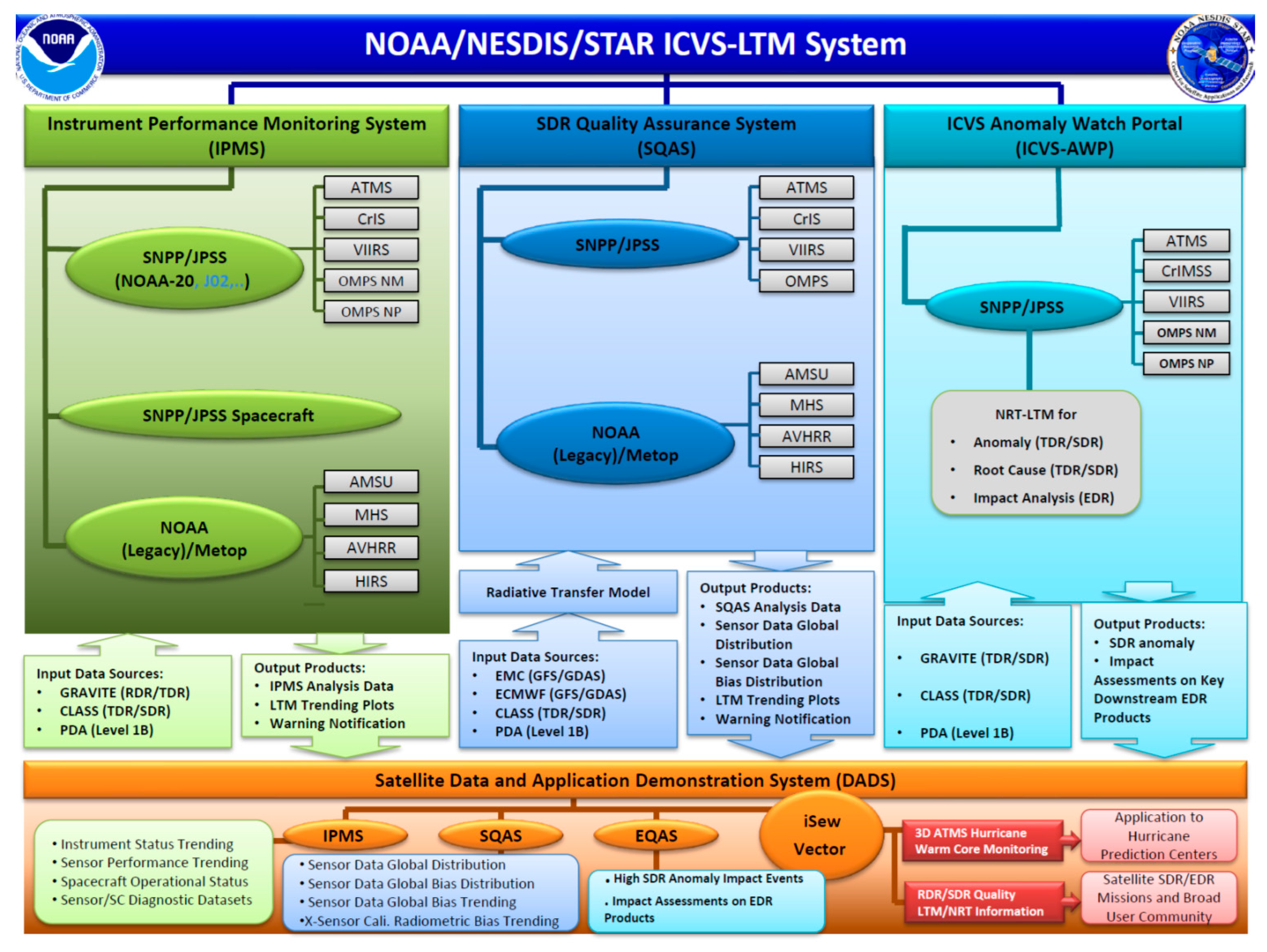
2.1. ICVS-LTM
2.2. Channels Characterizations for Four Instruments
2.3. Data
2.4. Two DD Methods
3. Development of the 32D-AD Method
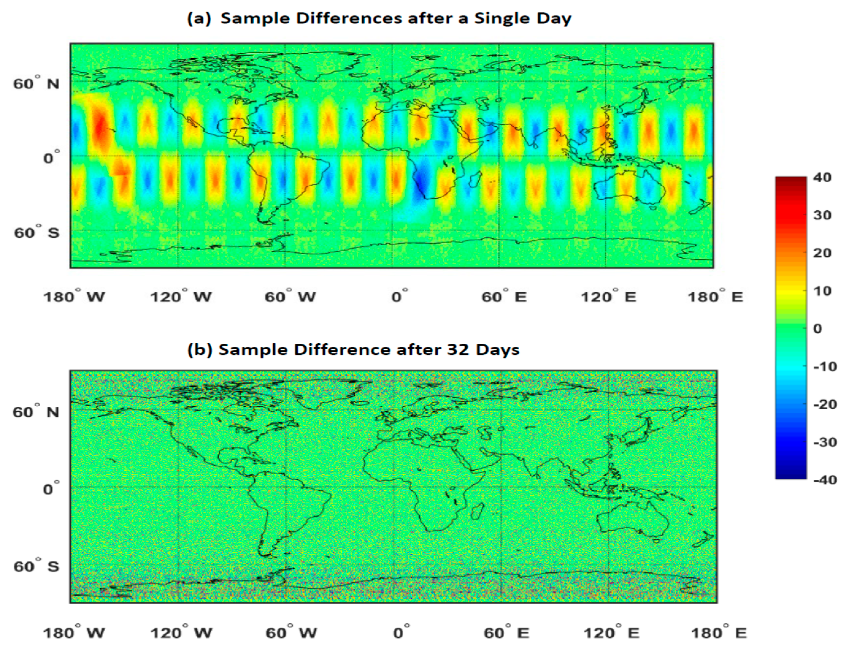
3.1. Principle of 32D-AD Method
3.2. Diurnal Error Sources
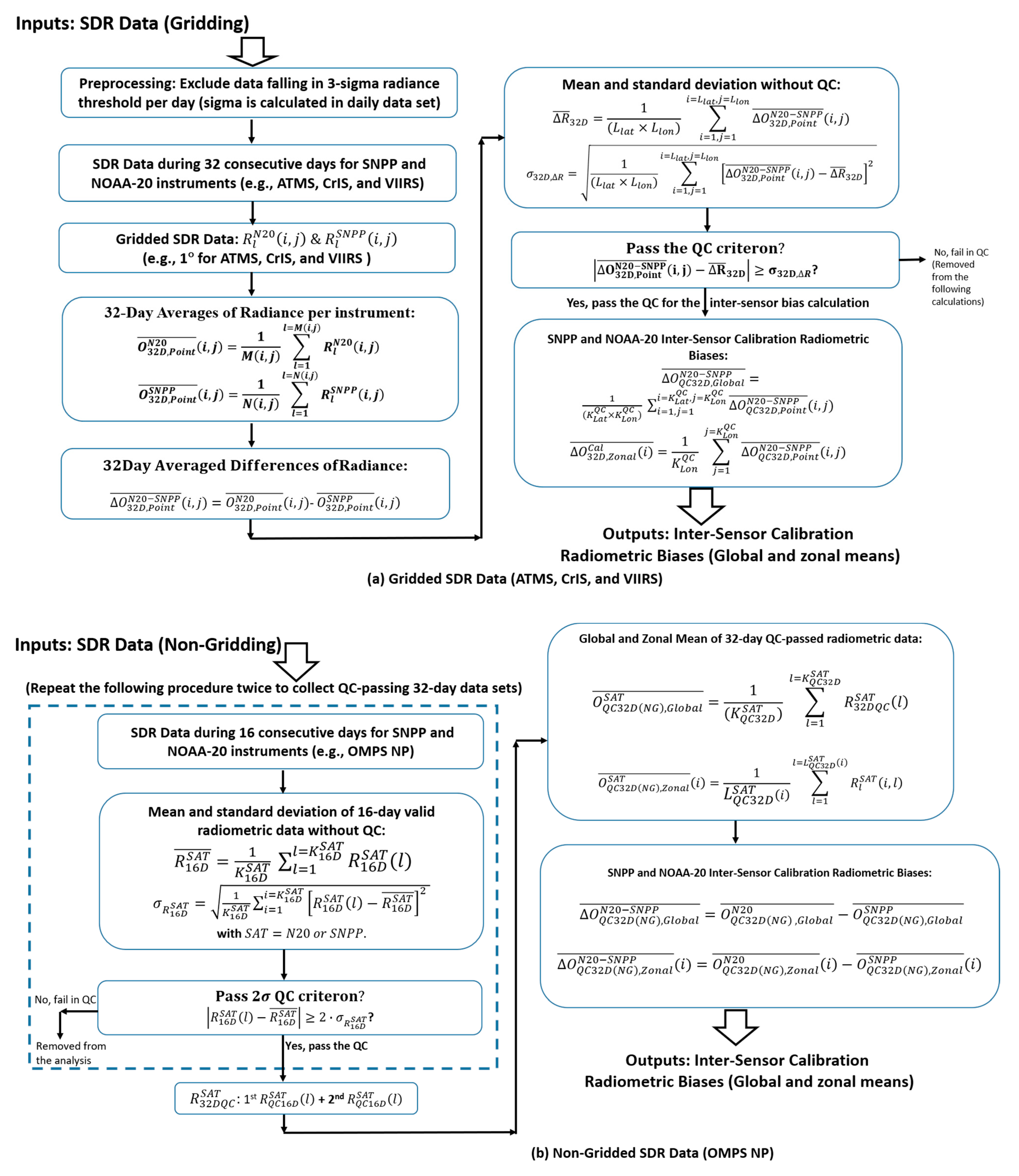
4. Calculation of Inter-Sensor Calibration Radiometric Biases Using the 32D-AD Method
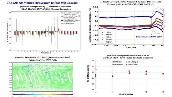
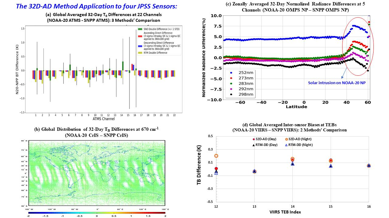
5. Application to Observations from SNPP and NOAA-20 Instruments within ICVS Framework
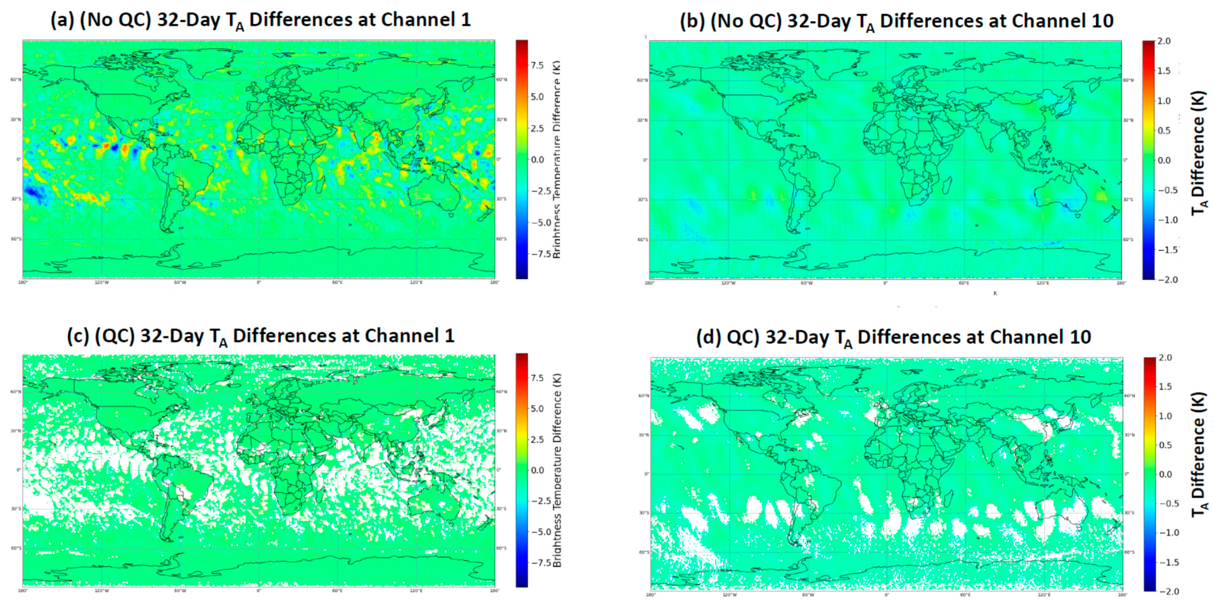
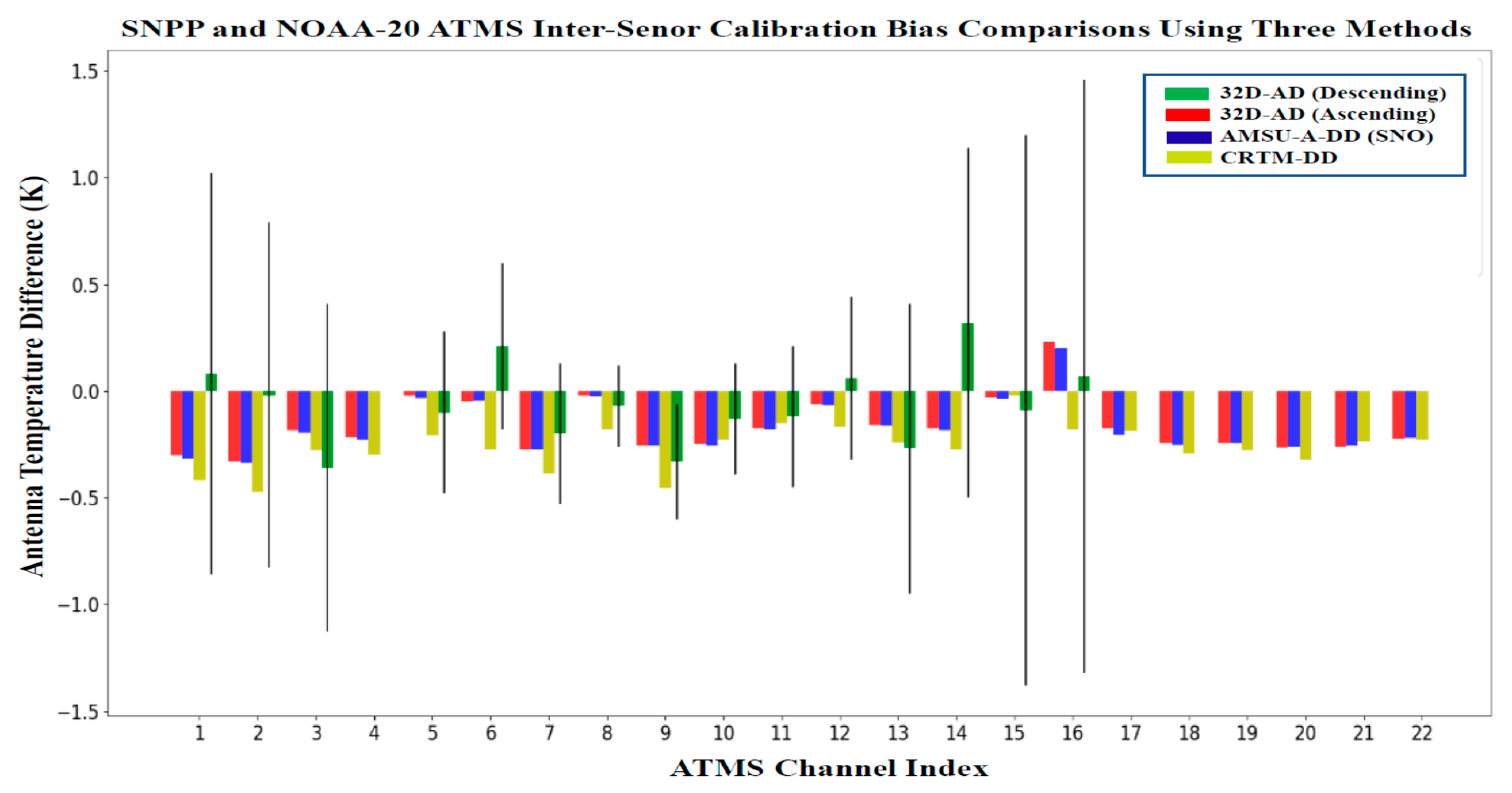
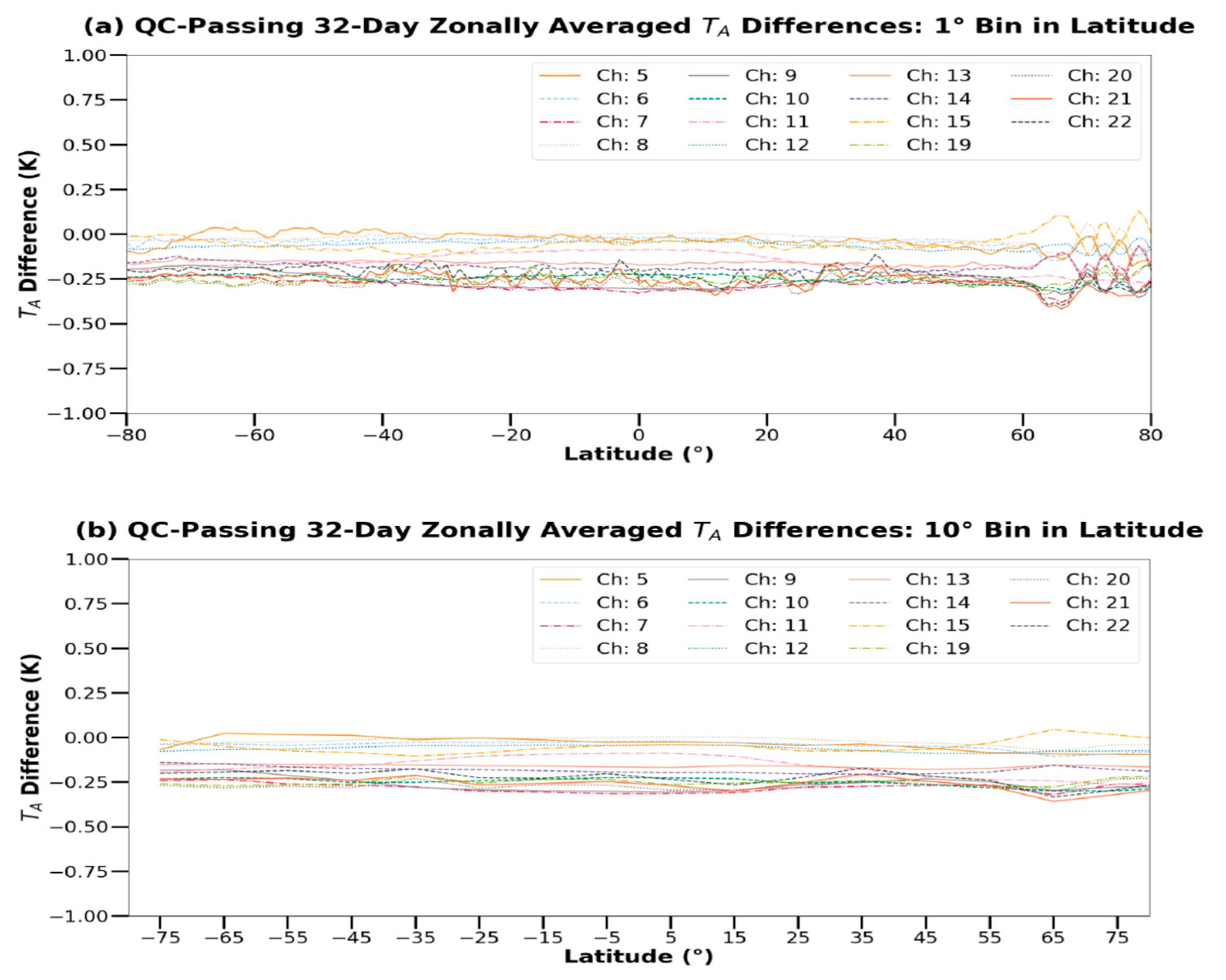
5.1. ATMS
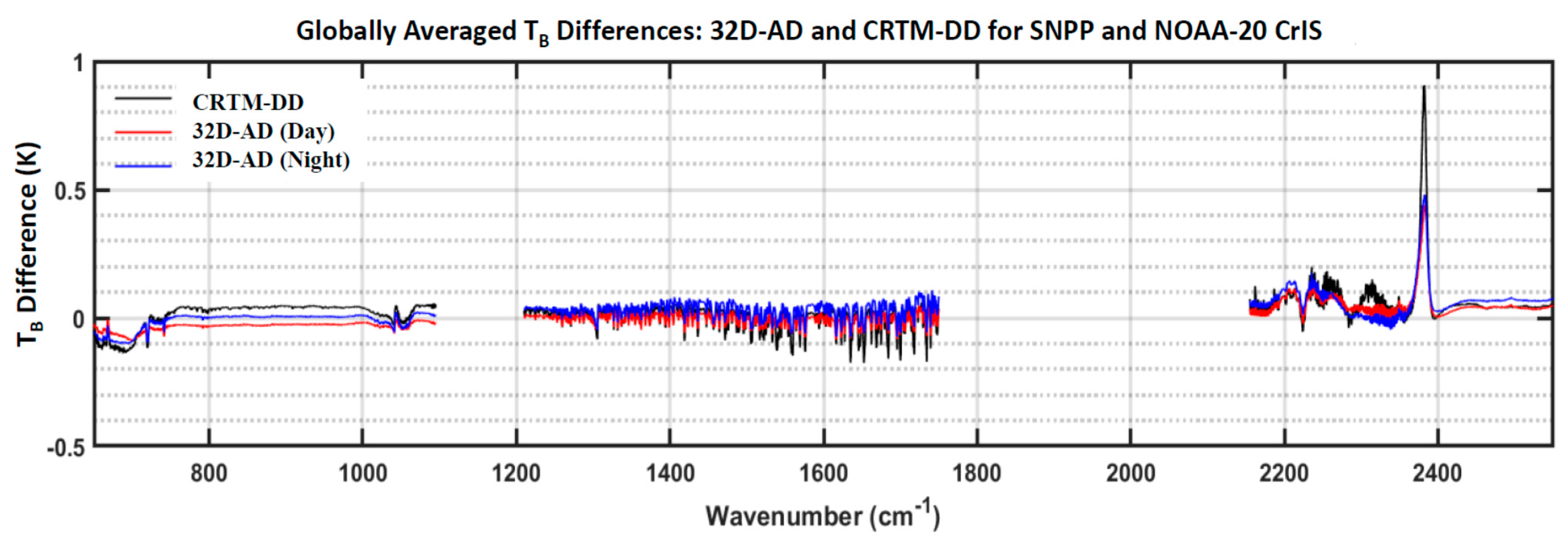
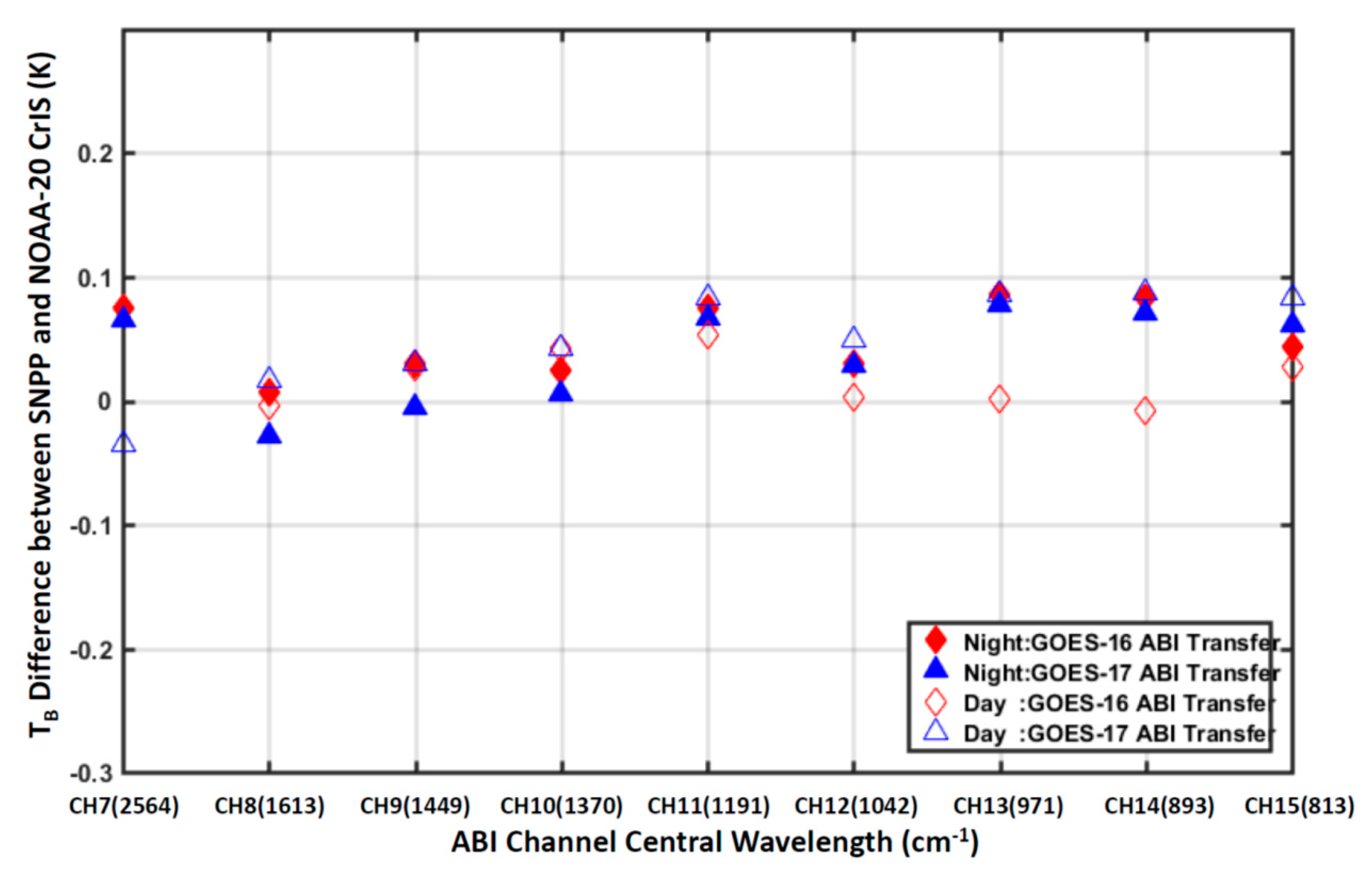
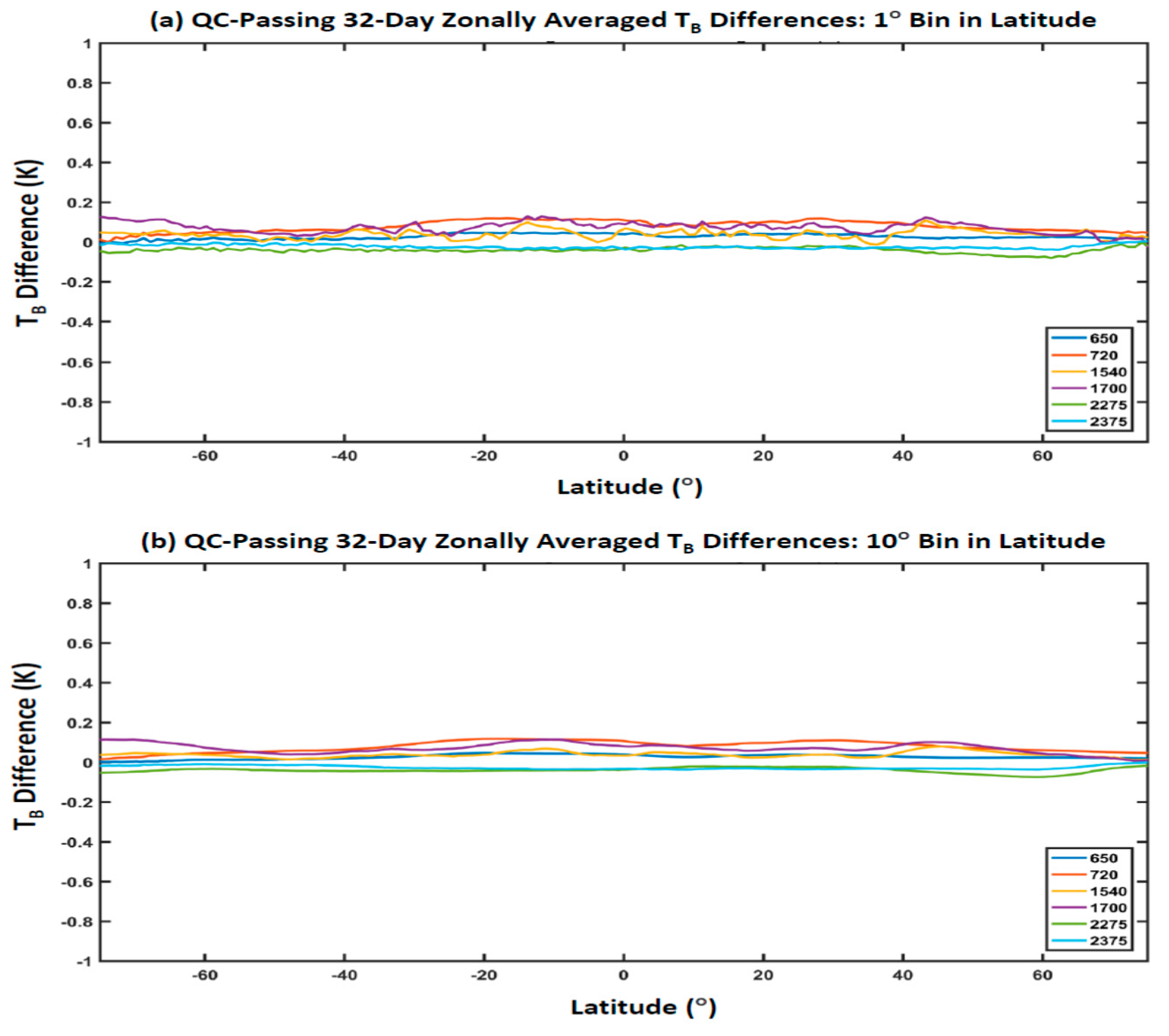
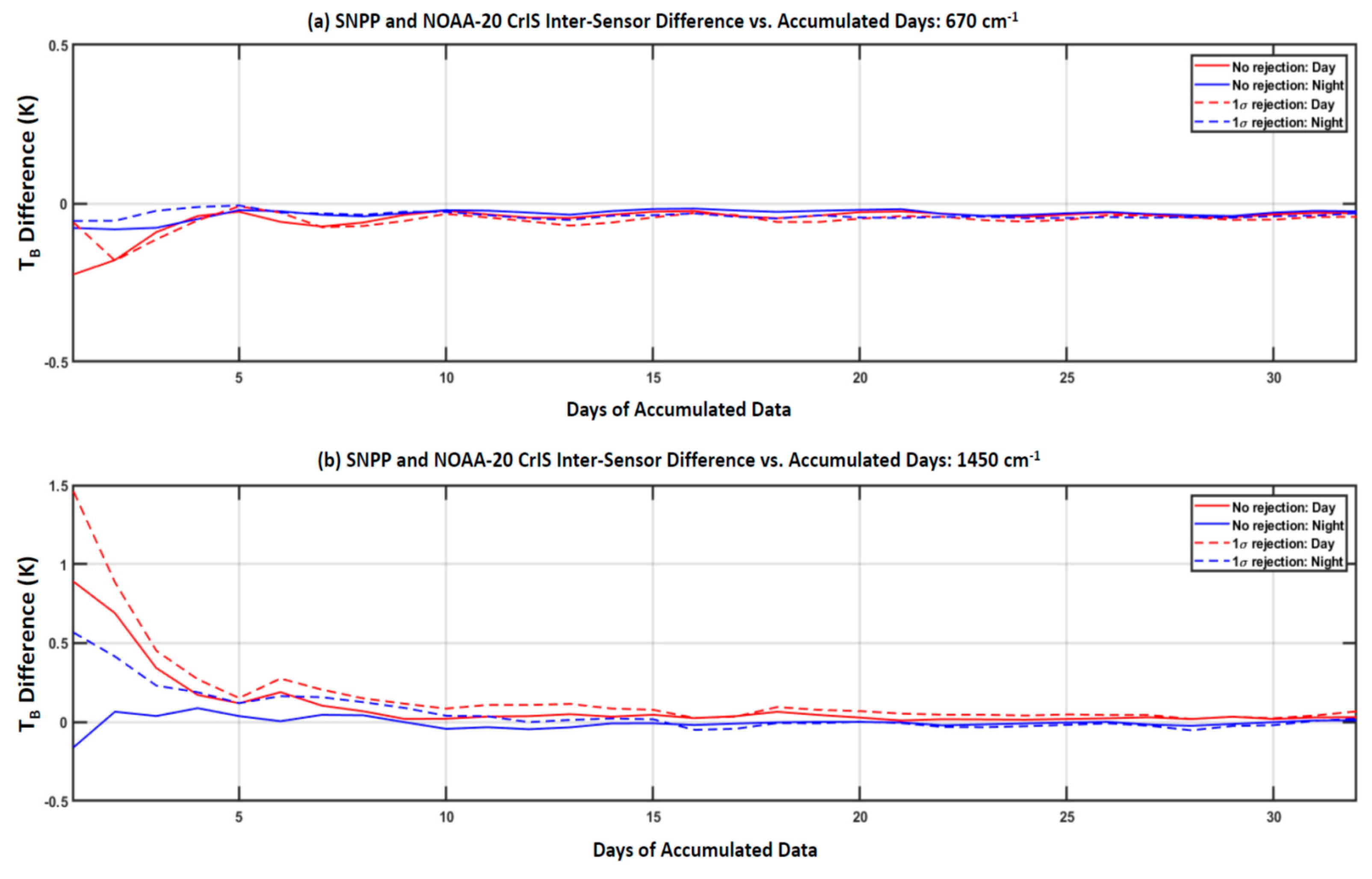
5.2. CrIS
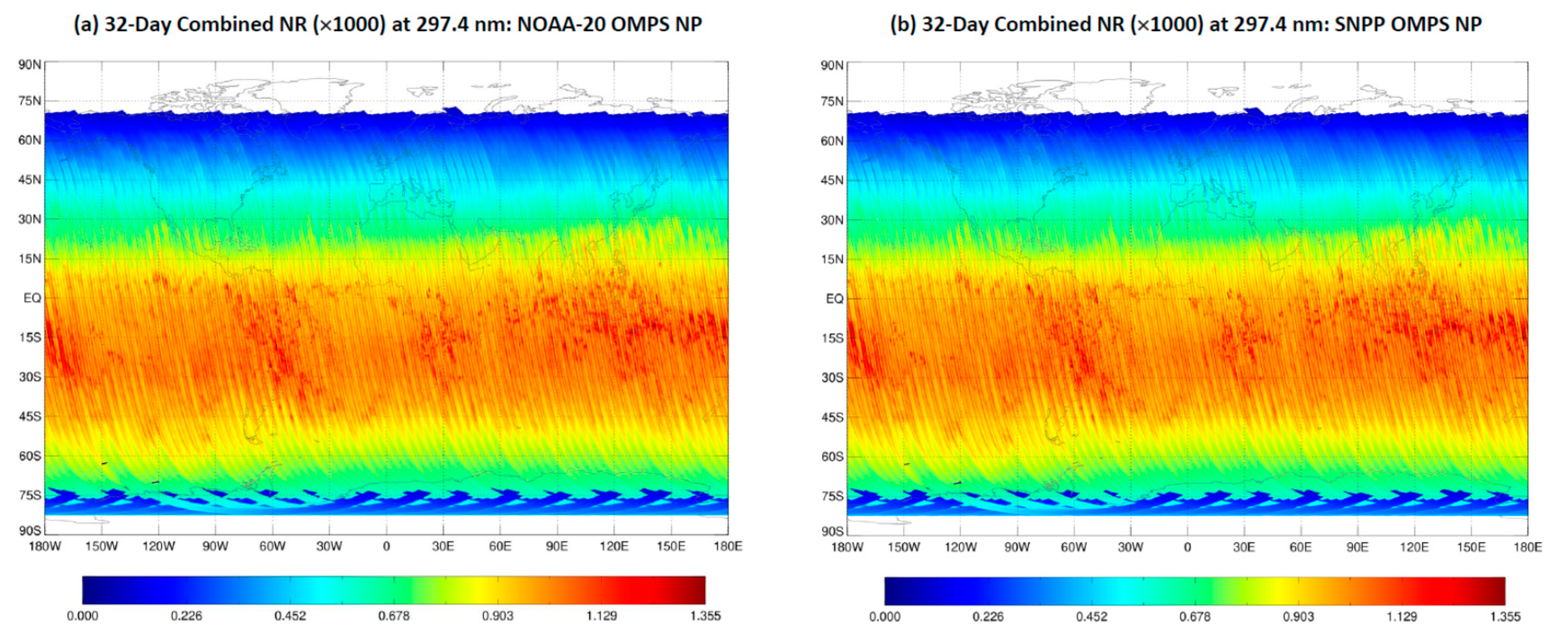
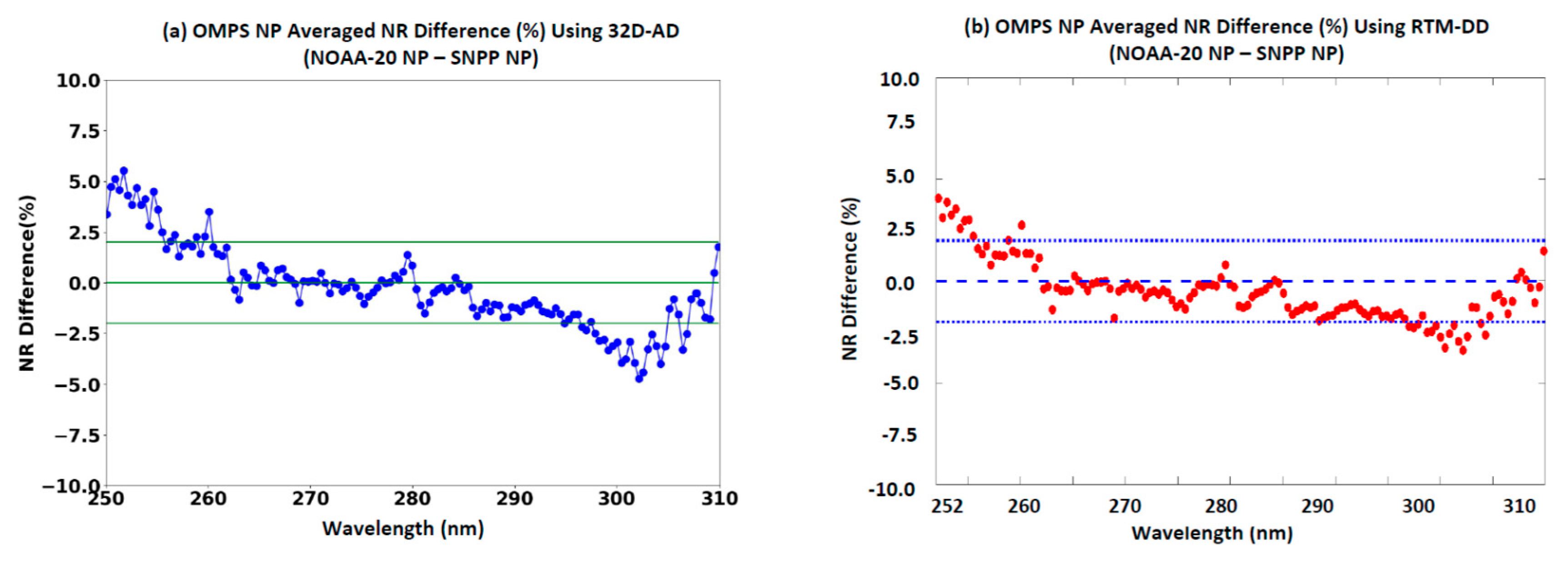
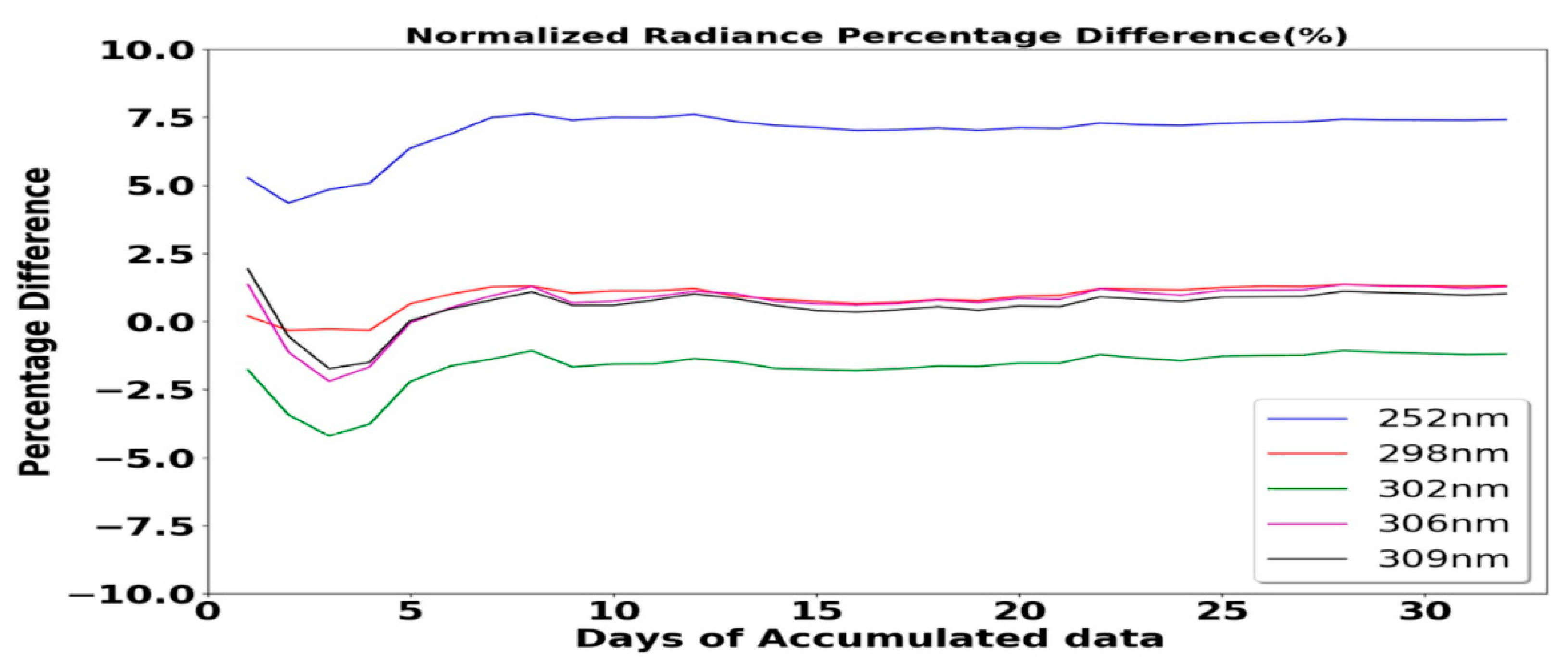
5.3. OMPS NP
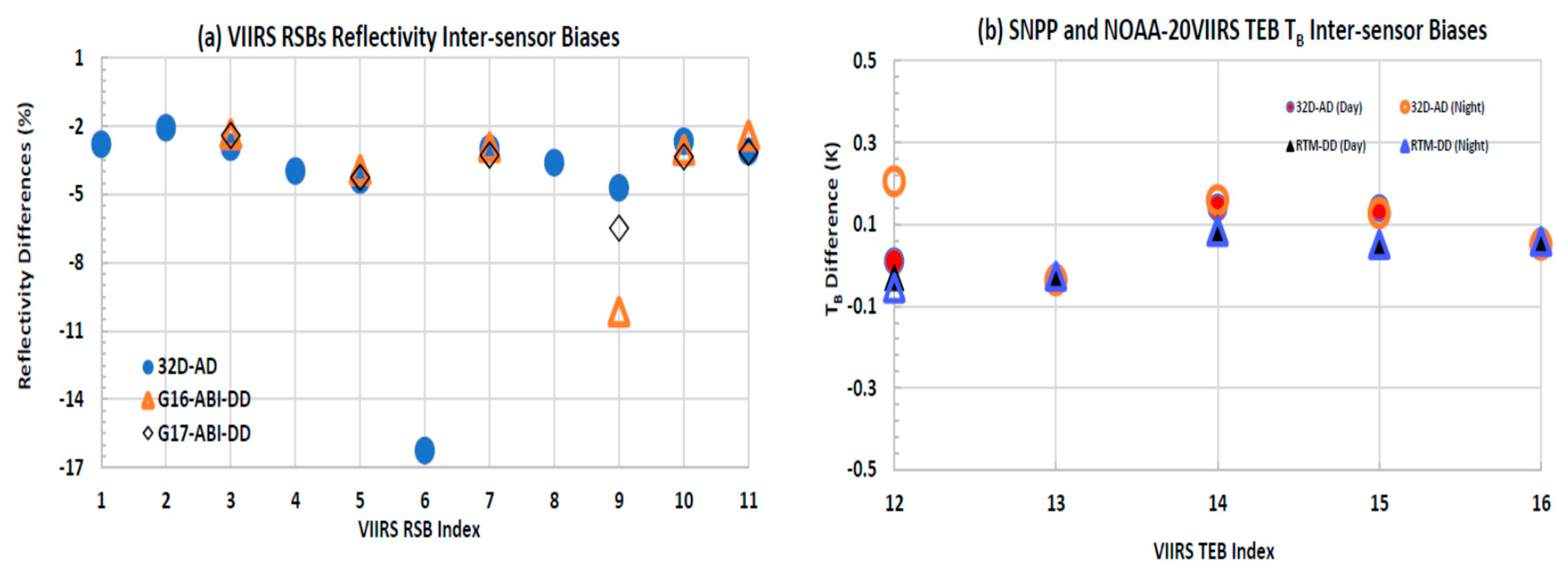
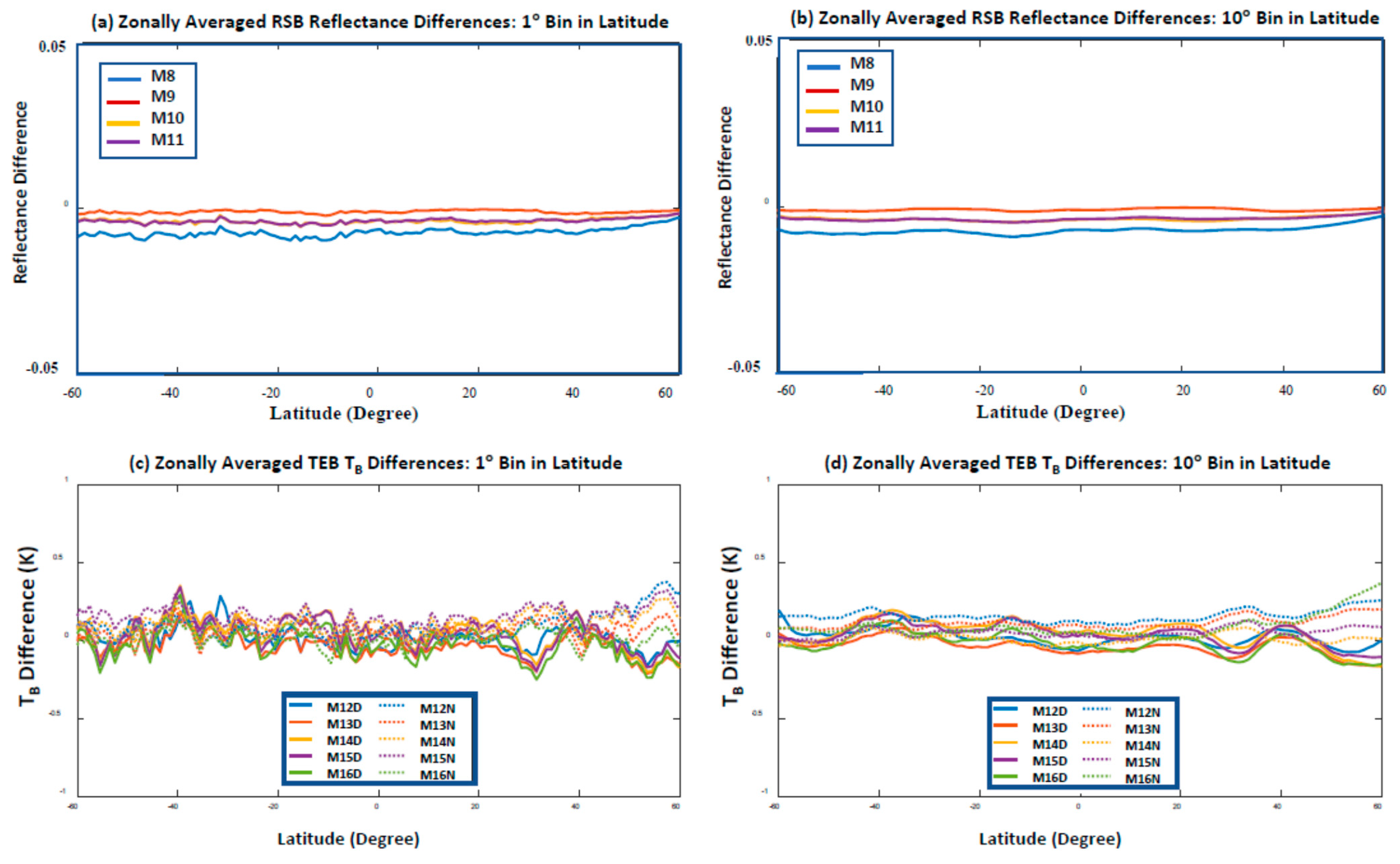
5.4. VIIRS
5.5. Some Discussions about 32D-AD Method
6. Summary and Conclusions
Author Contributions
Funding
Data Availability Statement
Acknowledgments
Conflicts of Interest
Appendix A. Detailed Descriptions of Variables in the 32D-AD Method

| 32-day-averaged differences (32D-AD) of gridded data at location for the same type of instruments between NOAA-20 and SNPP, referring to the individual 32D-AD at location | |
| Zonal mean difference of the 32-day gridded data at the ith latitude (range) for the same type of instruments between NOAA-20 and SNPP, referring to the zonal mean of 32D-AD | |
| Same as except for the QC-passing gridded data | |
| Same as except for the data without gridding | |
| Global mean difference of 32-day gridded data for the same type of instruments between NOAA-20 and SNPP, referring to the global mean of 32D-AD | |
| Same as except for the QC-passing gridded data | |
| Same as except for the data without gridding | |
| Same as except for the QC-passing data | |
| Global mean of the 32-day data without gridding per satellite, . | |
| Zonal mean of the 32-day data (no gridding) at a given latitude (range) per satellite | |
| Average of the 32-day gridded data at location per satellite | |
| lth data at the location among the 32-day gridded data per satellite | |
| lth data of accumulated 32-day datasets without gridding per satellite | |
| Sample size of the 32-day data without gridding per satellite | |
| Sample size of the 32-day QC-passing data without gridding per satellite | |
| Sample size of the 32-day data without gridding at the ith latitude (range) per satellite | |
| Same as except for the QC-passing data per satellite | |
| Sample size of the 32-day gridded data at the location by NOAA-20 instrument | |
| Same as except for the QC-passing gridded data per satellite | |
| Same as except for SNPP instrument | |
| and | is determined by the grid resolution of the data in latitude direction, e.g., for 1° × 1° gridded data; is the same as except for QC-passing data |
| and | is determined by the grid resolution of the data in longitude direction, e.g., for 1° × 1° gridded data; and is the same as except for QC-passing data |
Appendix B. 32D-AD Formulae for Estimating Inter-Sensor Calibration Radiometric Biases

References
- Yan, B.; Sun, N.; Jin, X.; Huang, J.; Liang, D.; Porter, W.; Liang, X.; Kireev, S.; Zhou, L.; Goldberg, M. Exploring New Developments of the STAR Integrated Calibration/Validation System; American Geophysical Union, Fall Meeting: Washington, DC, USA, 2018; Available online: https://ui.adsabs.harvard.edu/abs/2018AGUFM.A23A03B/abstract (accessed on 19 July 2021).
- Cao, C.; Weinreb, M.; Xu, H. Predicting simultaneous nadir overpasses among polar-orbiting meteorological satellites for the intersatellite calibration of radiometers. J. Atmos. Ocean. Technol. 2004, 21, 537–542. [Google Scholar] [CrossRef]
- Cao, C.; Weng, F.; Goldberg, M.; Wu, X.; Xu, H.; Ciren, P. Intersatellite calibration of polar-orbiting radiometers using the SNO/SCO method. In Proceedings of the 2005 IEEE International Geoscience and Remote Sensing Symposium, Seoul, Korea, 29 July 2005; p. 4. [Google Scholar] [CrossRef]
- Iacovazzi, R.; Cao, C. Reducing Uncertainties of SNO-Estimated Intersatellite AMSU-A Brightness Temperature Biases for Surface-Sensitive Channels. J. Atmos. Ocean. Technol. 2007, 25, 1048–1054. [Google Scholar] [CrossRef]
- Yan, B.; Weng, F. Intercalibration Between Special Sensor Microwave Imager/Sounder and Special Sensor Microwave Imager. IEEE Trans. Geosci. Remote. Sens. 2008, 46, 984–995. [Google Scholar]
- Yang, S.; Weng, F.; Yan, B.; Sun, N.; Goldberg, M. Special Sensor Microwave Imager (SSM/I) Intersensor Calibration Using a Simultaneous Conical Overpass Technique. J. Appl. Meteor. Climatol. 2011, 50, 77–95. [Google Scholar] [CrossRef]
- Yan, B.; Chen, J. Post-launch Performance Assessment of Metop-C Advanced Microwave Sounding Unit-A (AMSU-A) Instrument Noise and Antenna Temperature Data. In Proceedings of the 2020 IEEE International Geoscience and Remote Sensing Symposium, Waikoloa, HI, USA, 26 September–2 October 2020. [Google Scholar]
- Yan, B.; Chen, J.; Zou, C.-Z.; Ahmad, K.; Qian, H.; Garrett, K.; Zhu, T.; Han, D.; Green, J. Calibration and Validation of Antenna and Brightness Temperatures from Metop-C Advanced Microwave Sounding Unit-A (AMSU-A). Remote Sens. 2020, 12, 2978. [Google Scholar] [CrossRef]
- Uprety, S.; Cao, C.; Shao, X. Geo-Leo intercalibration to evaluate the radiometric performance of NOAA-20 VIIRS and GOES-16 ABI. In Proceedings of the SPIE Optical Engineering + Applications, San Diego, CA, USA, 9 September 2019. [Google Scholar] [CrossRef]
- Jin, X.; Yan, B.; Sun, N. Advancing CrIS and ABI Inter-Comparison Applicable for JSTAR Integrated Calibration/Validation System; AGU Fall meeting: Washington, DC, USA, 2019. [Google Scholar]
- Yan, B.; Weng, F. Effects of Microwave Desert Surface Emissivity on AMSU-A Data Assimilation. IEEE Trans. Geosci. Remote. Sens. 2011, 49, 1263–1276. [Google Scholar] [CrossRef]
- Jaross, G.; Huang, L.-K. Update on the NOAA-20 OMPS NP solar intrusion anomaly. In Proceedings of the NASA Ozone Processing Team (OPT) meeting, Greenbelt, MD, USA, 8 August 2020. [Google Scholar]
- Ramachandran, S.; Keegstra, P.; Vogel, R.L.; Soracco, M.; Hughes, K. Ocean color products validation at NOAA CoastWatch. In Proceedings of the 2014 IEEE Geoscience and Remote Sensing Symposium, Quebec City, QC, Canada, 13–18 July 2014; pp. 1182–1185. [Google Scholar] [CrossRef] [Green Version]
- Sungmin, O.; Kirstetter, P.-E. Evaluation of diurnal variation of GPM IMERG derived summer precipitation over the contiguous US using MRMS data. Q. J. R. Meteorol. Soc. 2018, 144, 270–281. [Google Scholar] [CrossRef] [Green Version]
- Zou, C.-Z.; Wang, W. 2009: Diurnal drift correction in the NESDIS/STAR MSU/AMSU atmospheric temperature climate data record. In Proceedings of the SPIE Optical Engineering + Applications, San Diego, CA, USA, 12 August 2009; Volume 7456. [Google Scholar]
- Po-Chedley, S.; Thorsen, T.J.; Fu, Q. Removing Diurnal Cycle Contamination in Satellite-Derived Tropospheric Temperatures: Understanding Tropical Tropospheric Trend Discrepancies. J. Clim. 2015, 28, 2274–2290. [Google Scholar] [CrossRef]
- Yan, B.; Goldberg, M.; Jin, X.; Huang, J.; Sun, N.; Liang, D.; Porter, W.; Zhou, L. SNPP and NOAA-20 Global Inter-Sensor Bias Assessments within ICVS Framework Using 32-Day Averaged Difference Method. In Proceedings of the 2020 IEEE International Geoscience and Remote Sensing Symposium, Virtual Symposium, Waikoloa, HI, USA, 26 September 2020. [Google Scholar]
- Huang, J.; Yan, B.; Sun, N.; Liang, D.; Porter, W.; Liang, X.; Jin, X.; Atkins, T.; Zhou, L.; Goldberg, M. JPSS/STAR ICVS Severe Event Watch System Development and Applications; American Geophysical Union, Fall Meeting: Washington, DC, USA, 2018; Available online: https://ui.adsabs.harvard.edu/abs/2018AGUFMIN33F0898H/abstract (accessed on 21 February 2021).
- Yan, B.; Liang, D.; Porter, W.; Huang, J.; Sun, N.; Zhou, L.; Zhu, T.; Goldberg, M.; Zhang, D.-L.; Liu, Q. Gap filling of advanced technology microwave sounder data as applied to hurricane warm core animations. Earth Space Sci. 2020, 7, e2019EA000961. [Google Scholar] [CrossRef]
- Joint Polar Satellite System (JPSS) Advanced Technology Microwave Sounder (ATMS) SDR Radiometric Calibration Algorithm Theoretical Basic Document (ATBD). 2011. Available online: https://www.star.nesdis.noaa.gov/jpss/documents/ATBD/D0001-M01-S01-001_JPSS_ATBD_ATMS-SDR_A.pdf (accessed on 30 March 2021).
- Rev, C. (Ed.) Joint Polar Satellite System (JPSS) Cross Track Infrared Sounder (CrIS) Sensor Data Records (SDR) Algorithm Theoretical Basis Document (ATBD); Code 474, 474-00032; Goddard Space Flight Center: Greenbelt, Maryland, 2014.
- Joint Polar Satellite System (JPSS) OMPS Nadir Profile Ozone Algorithm Theoretical Basis Document; JPSS Ground Project Code 474-00026; Goddard Space Flight Center: Greenbelt, Maryland, 2014.
- NOAA Technical Report NESDIS 142, Visible Infrared Imaging Radiometer Suite (VIIRS) Sensor Data Record (SDR) User’s Guide, Version 1.3, NOAA National Environmental Satellite, Data, and Information Service, 2017. Available online: https://ncc.nesdis.noaa.gov/documents/documentation/viirs-users-guide-tech-report-142a-v1.3.pdf (accessed on 24 March 2021).
- Yan, B.; Ahmad, K. Derivation and Validation of Sensor Brightness Temperatures for Advanced Microwave Sounding Unit-A Instruments. IEEE Trans. Geosci. Remote. Sens. 2020, 99, 1–11. [Google Scholar] [CrossRef]
- Weng, F.; Zou, X.; Sun, N.; Yang, H.; Tian, M.; Blackwell, W.J.; Wang, X.; Lin, L.; Anderson, K. Calibration of Suomi national polar-orbiting partnership advanced technology microwave sounder. J. Geophys. Res. Atmos. 2013, 118, 11187–11200. [Google Scholar] [CrossRef]
- Yan, B.; Pan, C.; Beck, T.; Xiong, X.; Liang, D.; Chen, J.; Jaross, G.; Flynn, L. NOAA-20 OMPS NP SDR Report for Validated Maturity Review. NOAA JPSS Science Review. 2020. Available online: https://www.star.nesdis.noaa.gov/jpss/documents/AMM/N20/OMPS_NP_SDR_Validated.pdf (accessed on 30 March 2021).
- Han, Y.; van Delst, P.; Liu, Q.; Weng, F.; Yan, B.; Treadon, R.; Derber, J. JCSDA Community Radiative Transfer Model (CRTM)-Version 1. NOAA Tech. Rep. NESDIS 2006, 122, 1–33. [Google Scholar]
- Chen, Y.; Weng, F.; Han, Y.; Liu, Q. Validation of the Community Radiative Transfer Model by using CloudSat data. J. Geophys. Res. Atmos. 2008, 113, D8. [Google Scholar] [CrossRef]
- Ding, S.; Yang, P.; Weng, F.; Liu, Q.; Han, Y.; van Delst, P.; Li, J.; Baum, B. Validation of the community radiative transfer model. J. Quant. Spectrosc. Radiat. Transf. 2011, 112, 1050–1064. [Google Scholar] [CrossRef]
- Carminat, F.; Migliorini1, S.; Ingleby, B.; Bell, W.; Lawrence, H.; Newman, S.; Hocking, J.; Smith, A. Using reference radiosondes to characterize NWP model uncertainty for improved satellite calibration and validation. Atmos. Meas. Tech. 2019, 12, 83–106. [Google Scholar] [CrossRef] [Green Version]
- Eck, F.; Bhartia, P.K.; Kerr, J.B. Satellite estimation of spectral UVB irradiance using TOMS derived total ozone and UV reflectivity. Geophys. Res. Lett. 1995, 22, 611–614. [Google Scholar] [CrossRef]
- Frank, W.; Schabel, M. Effects of orbital decay on satellite-derived lower-tropospheric temperature trends. Nature 1998, 394, 661–664. [Google Scholar]
- Han, Y.; Revercomb, H.; Cromp, M.; Gu, D.; Johnson, D.; Mooney, D.; Scott, D.; Strow, L.; Bingham, G.; Borg, L.; et al. Suomi NPP CrIS measurements, sensor data record algorithm, calibration and validation activities, and record data quality. J. Geophys. Res. Atmos. 2013, 118, 12734–12748. [Google Scholar] [CrossRef]
- Chen, Y.; Han, Y.; Weng, F. Characterization of long-term stability of Suomi NPP Cross-Track Infrared Sounder spectral calibration. IEEE Trans. Geosci. Remote. Sens. 2017, 55, 1147–1159. [Google Scholar] [CrossRef]
- Sanchez, F.; Tobin, D.; Strow, L.; Scott, D.; Mooney, D.; Johnson, D.; Suwinski, L.; Predina, J.; Bolen, D.; Guenther, B.; et al. NOAA-20 CrIS SDR Report for Validated Maturity Review. NOAA JPSS Science Review. 2018. Available online: https://www.star.nesdis.noaa.gov/jpss/documents/AMM/N20/CrIS_SDR_Validated.pdf (accessed on 17 March 2021).
- Sanchez, F.; Strow, L.; Tobin, D.; Scott, D.; Chen, Y.; Tremblay, D.; Knuteson, R.; Johnson, D.; Buttles, C.; Suwinski, L.; et al. SNPP CrIS Instrument: Successfully Restored after Midwave Infrared Band Anomaly, Submitted to the ITGRS. In Proceedings of the 22nd International TOVS Study Conference, Saint-Sauveur, QC, Canada, 31 October–6 November 2019. [Google Scholar]
- McClatchey, R.A.; Fenn, R.W.; Selby, J.E.A.; Volz, F.E.; Garing, J.S. Optical Properties of the Atmosphere; Research Paper 411, AFCRL-72-0497; Defense Technical Information Center: Fort Belvoir, VA, USA, 1972; p. 108.
- Sun, N.; Yan, B.; Liu, Q. Evaluation of Advanced Technology Microwave Sounder (ATMS) Science Data Long-Term Trending through Intersatellite Comparisons. In Proceedings of the 101st AMS Virtual Conference, Online, 10–15 January 2021. [Google Scholar]
- Jin, X.; Yan, B.; Sun, N. Improving SNPP and NOAA-20 CrIS LTM Inter-sensor Radiometric Bias Assessment by Using Interpolating ABI Measurements as Transfer. In Proceedings of the 101st AMS Virtual Conference, Online, 10–15 January 2021. [Google Scholar]
- Pan, C.; Weng, F.; Flynn, L. Spectral performance and calibration of the Suomi NPP OMPS Nadir Profiler sensor. Earth Space Sci. 2017, 4, 737–745. [Google Scholar] [CrossRef]
- Pan., C.; Cao, C.; Flynn, L.; Xiong, X.; Beach, E.; Zhou, L. Performance of OMPS Nadir Profilers’ Sensor Data Records. IEEE Trans. Geosci. Remote. Sens. 2020. [Google Scholar] [CrossRef]
- Flynn, L.; Long, C.; Wu, X.; Evans, R.; Beck, C.T.; Petropavlovskikh, I.; McConville, G.; Yu, W.; Zhang, Z.; Niu, J.; et al. Performance of the Ozone Mapping and Profiler Suite (OMPS) products. J. Geophys. Res. Atmos. 2014, 119, 6181–6195. [Google Scholar] [CrossRef]
- Niu, J.; Flynn, L.E.; Beck, T.; Zhang, Z.; Beach, E. Evaluation and Improvement of the Near-Real-Time Linear Fit SO2; Retrievals from Suomi NPP Ozone Mapping and Profiler Suite. IEEE Trans. Geosci. Remote. Sens. 2021. [Google Scholar] [CrossRef]
- Wang, W.; Cao, C.; Blonski, S.; Gu, Y.; Zhang, B. An Improved Method for VIIRS Radiance Limit Verification and Saturation Rollover Flagging. IEEE Trans. Geosci. Remote. Sens. 2021, in press. [Google Scholar] [CrossRef]
- Cao, C.; Deluccia, F.; Xiong, J.; Weng, F. NPP VIIRS SDR Postlaunch Calibration/Validation. Available online: https://ncc.nesdis.noaa.gov/documents/presentations/ams-viirs-sdr-calval-star-cao-01232012.pdf (accessed on 1 January 2012).
- Cao, C.; Xiong, J.; Blonski, S.; Liu, Q.; Uprety, S.; Shao, X.; Bai, Y.; Weng, F. Suomi NPP VIIRS sensor data record verification, validation, and long-term performance monitoring. J. Geophys. Res. Atmos. 2013, 118, 11664–11678. [Google Scholar] [CrossRef]
- Yan, B.; Kireev, S.V. A New Methodology on Noise Equivalent Differential Temperature Calculation for On-Orbit Advanced Microwave Sounding Unit—A Instrument. IEEE Trans. Geosci. Remote. Sens. 2021. [Google Scholar] [CrossRef]
- Yan, B.; Chen, J.; Porter, W.; Kireev, S.; Sun, N.; Zou, C.; Zhou, L. Accurately Quantifying NEDT Performance for In-Orbit AMSU-A and ATMS Instruments by Using a Newly Developed Algorithm. In Proceedings of the 2019 Joint Satellite Conference, Boston, MA, USA, 28 September–4 October 2019. [Google Scholar]


| ATMS (GHz) | 23.8 (CH.1) | 31.4 (CH.2) | 50.3 (CH3) | 51.76 (CH4) | 52.8 (CH5) | 53.596 ± 0.115 (CH6) |
| 54.4 (CH7) | 54.94 (CH8) | 55.50 (CH9) | fo = 57.29 (CH10) | fo ± 0.217 (CH11) | fo ± 0.322 ± 0.048 (CH12) | |
| fo ± 0.322 ± 0.022 (CH13) | fo ± 0.322 ± 0.010 (CH14) | fo ± 0.322 ± 0.004 (CH15) | 88.2 (CH16) | |||
| 165.5 (CH17) | 183.31 ± 7.0 (CH18) | 183.31 ± 3.0 (CH20) | 183.31 ± 1.8 (CH21) | 183.31 ± 1.0 (CH22) | ||
| CrIS | LW: 650–1095 cm−1 (15.38–9.14 μm) | |||||
| MW: 1210–1750 cm−1 (8.26–5.71 μm) | ||||||
| SW: 2155–2550 cm−1 (4.64–3.92 μm) | ||||||
| OMPS NP | 250–310 nm (147 channels in a spectral resolution of ~0.41 nm) | |||||
| VIIRS (μm) | 0.412 (M1) | 0.445 (M2) | 0.488 (M3) | 0.555 (M4) | 0.672 (M5) | 0.746 (M6) |
| 0.865 (M7) | 1.24 (M8) | 1.378 (M9) | 1.61 (M10) | 2.25 (M11) | 3.70 (M12) | |
| 4.05 (M13) | 8.55 (M14) | 10.763 (M15) | 12.013 (M16) | |||
| 0.640 (I1) | 0.865 (I2) | 1.61 (I3) | 3.74 (I4) | 11.450 (I5) | 0.7 (DNB) | |
Publisher’s Note: MDPI stays neutral with regard to jurisdictional claims in published maps and institutional affiliations. |
© 2021 by the authors. Licensee MDPI, Basel, Switzerland. This article is an open access article distributed under the terms and conditions of the Creative Commons Attribution (CC BY) license (https://creativecommons.org/licenses/by/4.0/).
Share and Cite
Yan, B.; Goldberg, M.; Jin, X.; Liang, D.; Huang, J.; Porter, W.; Sun, N.; Zhou, L.; Pan, C.; Iturbide-Sanchez, F.; et al. A New 32-Day Average-Difference Method for Calculating Inter-Sensor Calibration Radiometric Biases between SNPP and NOAA-20 Instruments within ICVS Framework. Remote Sens. 2021, 13, 3079. https://doi.org/10.3390/rs13163079
Yan B, Goldberg M, Jin X, Liang D, Huang J, Porter W, Sun N, Zhou L, Pan C, Iturbide-Sanchez F, et al. A New 32-Day Average-Difference Method for Calculating Inter-Sensor Calibration Radiometric Biases between SNPP and NOAA-20 Instruments within ICVS Framework. Remote Sensing. 2021; 13(16):3079. https://doi.org/10.3390/rs13163079
Chicago/Turabian StyleYan, Banghua, Mitch Goldberg, Xin Jin, Ding Liang, Jingfeng Huang, Warren Porter, Ninghai Sun, Lihang Zhou, Chunhui Pan, Flavio Iturbide-Sanchez, and et al. 2021. "A New 32-Day Average-Difference Method for Calculating Inter-Sensor Calibration Radiometric Biases between SNPP and NOAA-20 Instruments within ICVS Framework" Remote Sensing 13, no. 16: 3079. https://doi.org/10.3390/rs13163079