Is Accurate Synoptic Altimetry Achievable by Means of Interferometric GNSS-R?

 , , , , , and
Abstract
:1. Introduction
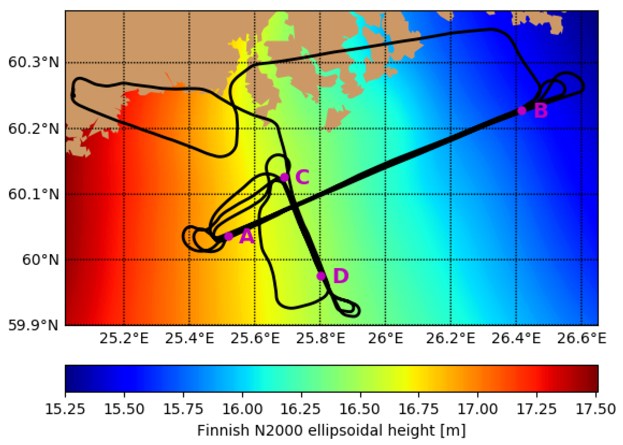
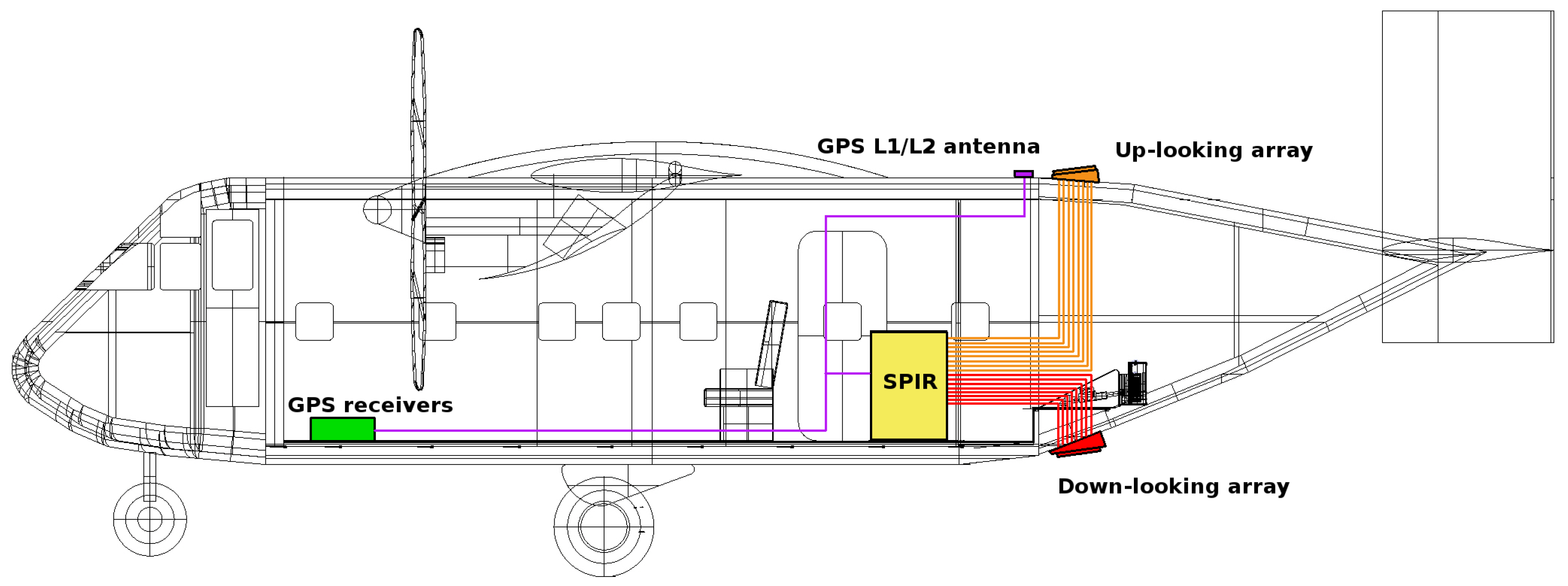
2. SPIR Campaign
3. Data Processing and Inversion
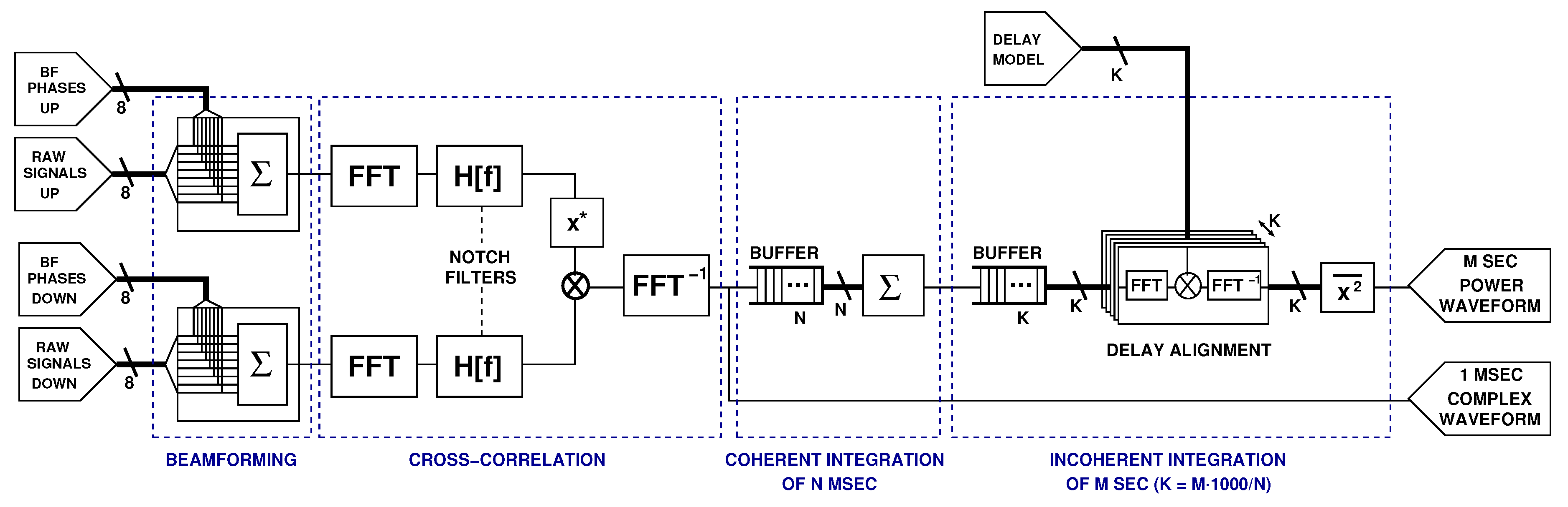
3.1. From Raw Signals to Power Waveforms
3.2. Delay Model
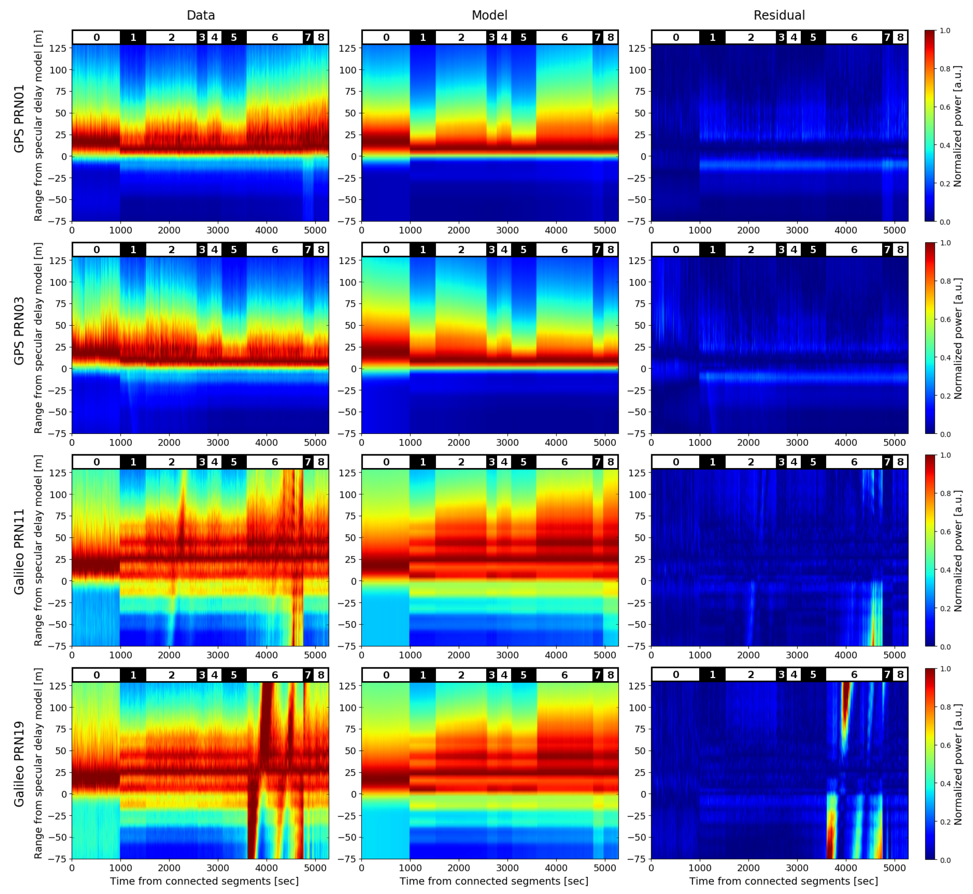
3.3. Waveform Model
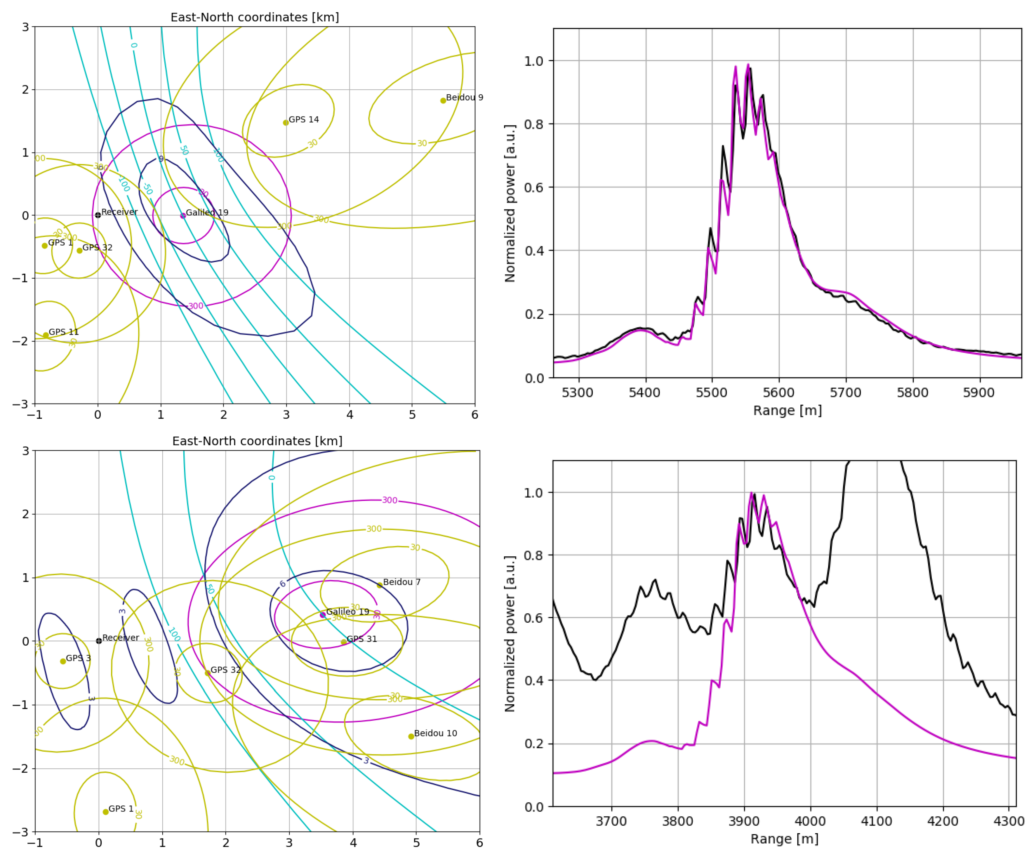
3.4. Primary Observable: Specular Delay
3.5. Altimetry Inversion
4. Results and Discussion
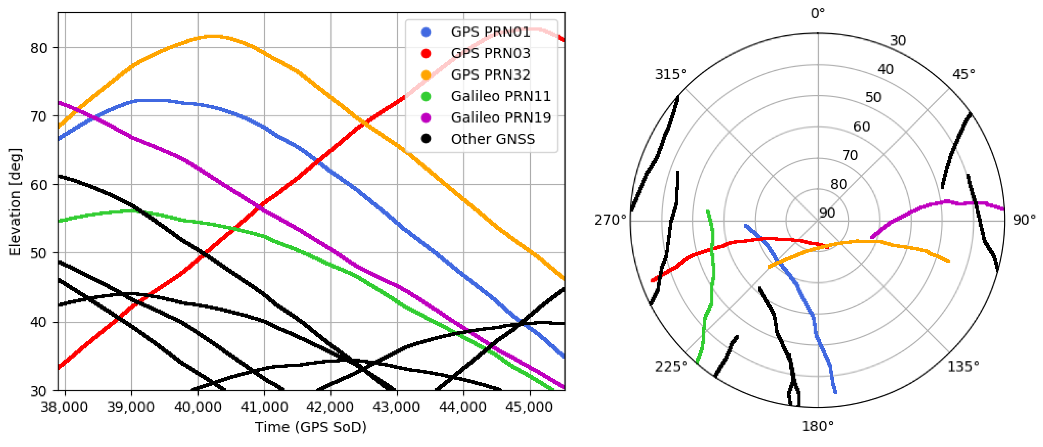
4.1. Preliminary Considerations
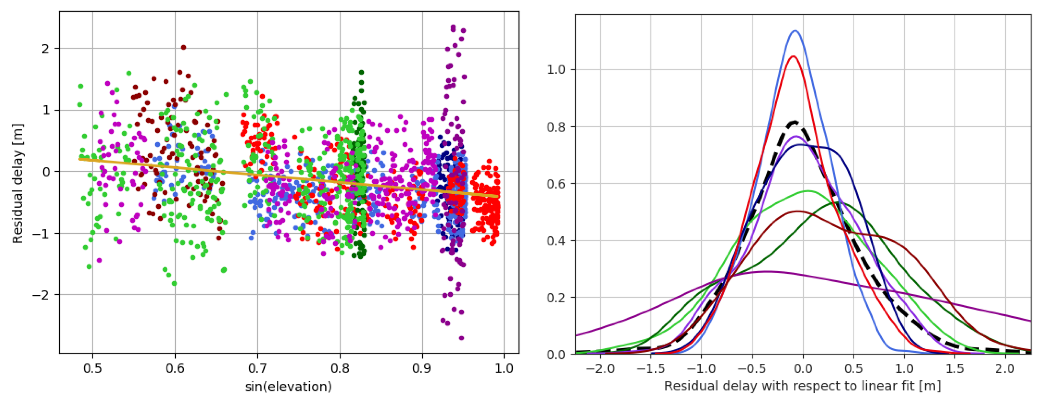
4.2. Specular Delay Analysis
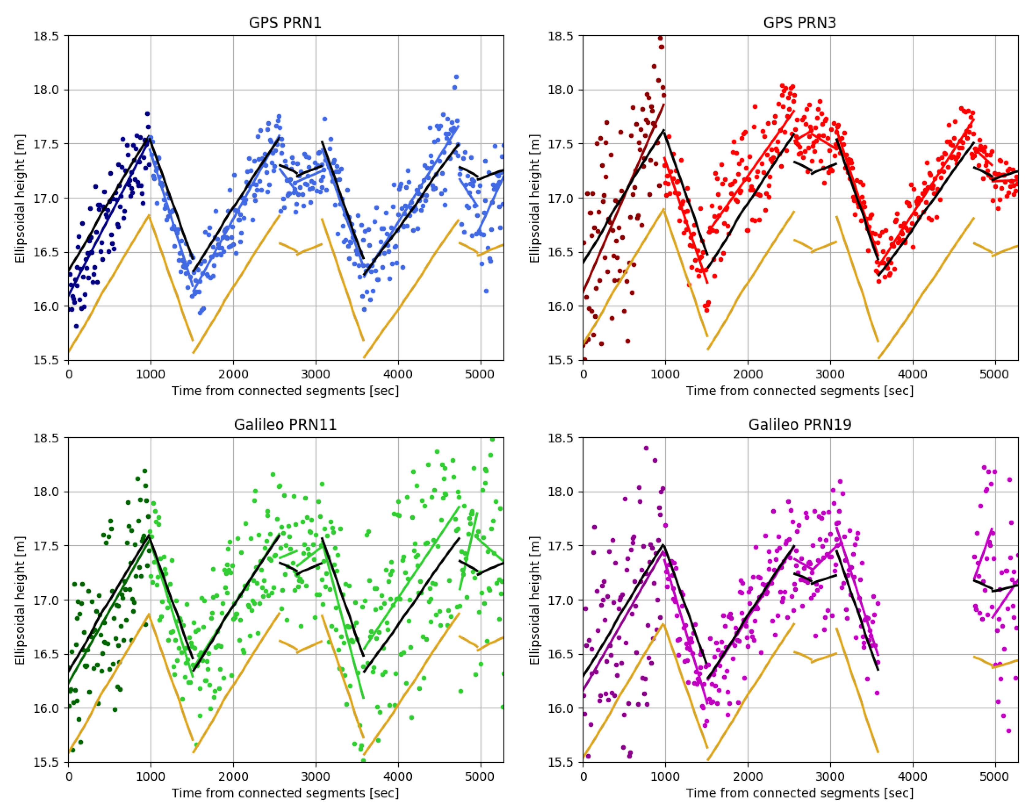
4.3. Altimetry Analysis
5. Conclusions
Author Contributions
Funding
Acknowledgments
Conflicts of Interest
References
- Martín-Neira, M. A passive reflectometry and interferometry system (PARIS): Application to ocean altimetry. ESA J. 1993, 17, 331–355. [Google Scholar]
- Cardellach, E.; Fabra, F.; Nogués-Correig, O.; Oliveras, S.; Ribó, S.; Rius, A. GNSS-R ground-based and airborne campaigns for ocean, land, ice, and snow techniques: Application to the GOLD-RTR data sets. Radio Sci. 2011, 46, 1–16. [Google Scholar] [CrossRef]
- Zavorotny, V.U.; Gleason, S.; Cardellach, E.; Camps, A. Tutorial on Remote Sensing Using GNSS Bistatic Radar of Opportunity. IEEE Geosci. Remote Sens. Mag. 2014, 2, 8–45. [Google Scholar] [CrossRef] [Green Version]
- Jin, S.; Cardellach, E.; Xie, F. GNSS Remote Sensing: Theory, Methods and Applications; Remote Sensing and Digital Image Processing; Springer: Dutch, The Netherlands, 2014. [Google Scholar] [CrossRef]
- Gleason, S.; Hodgart, S.; Sun, Y.; Gommenginger, C.; Mackin, S.; Adjrad, M.; Unwin, M. Detection and Processing of bistatically reflected GPS signals from low Earth orbit for the purpose of ocean remote sensing. IEEE Trans. Geosci. Remote Sens. 2005, 43, 1229–1241. [Google Scholar] [CrossRef] [Green Version]
- Unwin, M.; Jales, P.; Tye, J.; Gommenginger, C.; Foti, G.; Rosello, J. Spaceborne GNSS-Reflectometry on TechDemoSat-1: Early Mission Operations and Exploitation. IEEE J. Sel. Top. Appl. Earth Obs. Remote Sens. 2016, 9, 4525–4539. [Google Scholar] [CrossRef]
- Ruf, C.S.; Atlas, R.; Chang, P.S.; Clarizia, M.P.; Garrison, J.L.; Gleason, S.; Katzberg, S.J.; Jelenak, Z.; Johnson, J.T.; Majumdar, S.J.; et al. New Ocean Winds Satellite Mission to Probe Hurricanes and Tropical Convection. Bull. Am. Meteorol. Soc. 2016, 97, 385–395. [Google Scholar] [CrossRef]
- Lowe, S.T.; LaBrecque, J.L.; Zuffada, C.; Romans, L.J.; Young, L.E.; Hajj, G.A. First spaceborne observation of an Earth-reflected GPS signal. Radio Sci. 2002, 37, 1–28. [Google Scholar] [CrossRef]
- Carreno-Luengo, H.; Lowe, S.; Zuffada, C.; Esterhuizen, S.; Oveisgharan, S. Spaceborne GNSS-R from the SMAP Mission: First Assessment of Polarimetric Scatterometry over Land and Cryosphere. Remote Sens. 2017, 9, 362. [Google Scholar] [CrossRef]
- Clarizia, M.P.; Ruf, C.; Cipollini, P.; Zuffada, C. First spaceborne observation of sea surface height using GPS-Reflectometry. Geophys. Res. Lett. 2015, 43, 767–774. [Google Scholar] [CrossRef]
- Hu, C.; Benson, C.; Rizos, C.; Qiao, L. Single-Pass Sub-Meter Space-Based GNSS-R Ice Altimetry: Results From TDS-1. IEEE J. Sel. Top. Appl. Earth Obs. Remote Sens. 2017, 10, 3782–3788. [Google Scholar] [CrossRef]
- Li, W.; Cardellach, E.; Fabra, F.; Rius, A.; Ribó, S.; Martín-Neira, M. First spaceborne phase altimetry over sea ice using TechDemoSat-1 GNSS-R signals. Geophys. Res. Lett. 2017, 44, 8369–8376. [Google Scholar] [CrossRef]
- Rius, A.; Cardellach, E.; Fabra, F.; Li, W.; Ribó, S.; Hernández-Pajares, M. Feasibility of GNSS-R Ice Sheet Altimetry in Greenland Using TDS-1. Remote Sens. 2017, 9, 742. [Google Scholar] [CrossRef]
- Cartwright, J.; Clarizia, M.P.; Cipollini, P.; Banks, C.J.; Srokosz, M. Independent DEM of Antarctica Using GNSS-R Data From TechDemoSat-1. Geophys. Res. Lett. 2018, 45, 6117–6123. [Google Scholar] [CrossRef]
- Mashburn, J.; Axelrad, P.; Lowe, S.T.; Larson, K.M. Global Ocean Altimetry with GNSS Reflections from TechDemoSat-1. IEEE Trans. Geosci. Remote Sens. 2018, 56, 4088–4097. [Google Scholar] [CrossRef]
- Li, W.; Cardellach, E.; Fabra, F.; Ribó, S.; Rius, A. Lake Level and Surface Topography Measured with Spaceborne GNSS-Reflectometry from CYGNSS Mission: Example for the Lake Qinghai. Geophys. Res. Lett. 2018, 45, 13332–13341. [Google Scholar] [CrossRef]
- Ribó, S.; Arco, J.C.; Oliveras, S.; Cardellach, E.; Rius, A.; Buck, C. Experimental Results of an X-Band PARIS Receiver Using Digital Satellite TV Opportunity Signals Scattered on the Sea Surface. IEEE Trans. Geosci. Remote Sens. 2014, 52, 5704–5711. [Google Scholar] [CrossRef]
- Shah, R.; Garrison, J.L. Precision of Ku-Band Reflected Signals of Opportunity Altimetry. IEEE Geosci. Remote Sens. Lett. 2017, 14, 1840–1844. [Google Scholar] [CrossRef]
- Martín-Neira, M.; D’Addio, S.; Buck, C.; Floury, N.; Prieto-Cerdeira, R. The PARIS Ocean Altimeter In-Orbit Demonstrator. IEEE Trans. Geosci. Remote Sens. 2011, 49, 2209–2237. [Google Scholar] [CrossRef]
- Wickert, J.; Cardellach, E.; Martín-Neira, M.; Bandeiras, J.; Bertino, L.; Andersen, O.B.; Camps, A.; Catarino, N.; Chapron, B.; Fabra, F.; et al. GEROS-ISS: GNSS REflectometry, Radio Occultation, and Scatterometry Onboard the International Space Station. IEEE J. Sel. Top. Appl. Earth Obs. Remote Sens. 2016, 9, 4552–4581. [Google Scholar] [CrossRef] [Green Version]
- Cardellach, E.; Wickert, J.; Baggen, R.; Benito, J.; Camps, A.; Catarino, N.; Chapron, B.; Dielacher, A.; Fabra, F.; Flato, G.; et al. GNSS Transpolar Earth Reflectometry exploriNg System (G-TERN): Mission Concept. IEEE Access 2018, 6, 13980–14018. [Google Scholar] [CrossRef]
- Rius, A.; Nogués-Correig, O.; Ribó, S.; Cardellach, E.; Oliveras, S.; Valencia, E.; Park, H.; Tarongí, J.M.; Camps, A.; van der Marel, H.; et al. Altimetry with GNSS-R interferometry: First proof of concept experiment. GPS Solut. 2012, 16, 231–241. [Google Scholar] [CrossRef]
- Cardellach, E.; Rius, A.; Martín-Neira, M.; Fabra, F.; Nogués-Correig, O.; Ribó, S.; Kainulainen, J.; Camps, A.; D’Addio, S. Consolidating the Precision of Interferometric GNSS-R Ocean Altimetry Using Airborne Experimental Data. IEEE Trans. Geosci. Remote Sens. 2014, 52, 4992–5004. [Google Scholar] [CrossRef]
- Ribó, S.; Arco-Fernández, J.C.; Cardellach, E.; Fabra, F.; Li, W.; Nogués-Correig, O.; Rius, A.; Martín-Neira, M. A Software-Defined GNSS Reflectometry Recording Receiver with Wide-Bandwidth, Multi-Band Capability and Digital Beam-Forming. Remote Sens. 2017, 9, 450. [Google Scholar] [CrossRef]
- Bilker-Koivula, M. Development of the Finnish Height Conversion Surface FIN2005N00. Nord. J. Surv. Real Estate Res. 2010, 7, 76–88. [Google Scholar]
- Natural Resources Canada. Canadian Spatial Reference System—Precise Point Positioning Service. Available online: https://webapp.geod.nrcan.gc.ca/geod/tools-outils/ppp (accessed on 21 December 2015).
- Finnish Meteorological Institute. Theoretical Mean Sea Level at Finland. Available online: http://en.ilmatieteenlaitos.fi/theoretical-mean-sea-level (accessed on 6 May 2016).
- Rius, A.; Cardellach, E.; Martín-Neira, M. Altimetric Analysis of the Sea-Surface GPS-Reflected Signals. IEEE Trans. Geosci. Remote Sens. 2010, 48, 2119–2127. [Google Scholar] [CrossRef]
- Zavorotny, V.U.; Voronovich, A.G. Scattering of GPS signals from the ocean with wind remote sensing application. IEEE Trans. Geosci. Remote Sens. 2000, 38, 951–964. [Google Scholar] [CrossRef]
- Pierdicca, N.; Guerriero, L.; Brogioni, M.; Egido, A. On the coherent and non coherent components of bare and vegetated terrain bistatic scattering: Modelling the GNSS-R signal over land. In Proceedings of the 2012 IEEE International Geoscience and Remote Sensing Symposium, Munich, Germany, 22–27 July 2012; pp. 3407–3410. [Google Scholar] [CrossRef]
- Arroyo, A.A.; Camps, A.; Aguasca, A.; Forte, G.F.; Monerris, A.; Rüdiger, C.; Walker, J.P.; Park, H.; Pascual, D.; Onrubia, R. Dual-Polarization GNSS-R Interference Pattern Technique for Soil Moisture Mapping. IEEE J. Sel. Top. Appl. Earth Obs. Remote Sens. 2014, 7, 1533–1544. [Google Scholar] [CrossRef]
- Katzberg, S.J.; Torres, O.; Ganoe, G. Calibration of reflected GPS for tropical storm wind speed retrievals. Geophys. Res. Lett. 2006, 33, L18602. [Google Scholar] [CrossRef]
- Li, W.; Rius, A.; Fabra, F.; Cardellach, E.; Ribó, S.; Martín-Neira, M. Revisiting the GNSS-R Waveform Statistics and Its Impact on Altimetric Retrievals. IEEE Trans. Geosci. Remote Sens. 2018, 56, 2854–2871. [Google Scholar] [CrossRef]
- Pascual, D.; Park, H.; Onrubia, R.; Arroyo, A.; Querol, J.; Camps, A. Crosstalk Statistics and Impact in Interferometric GNSS-R. IEEE J. Sel. Top. Appl. Earth Obs. Remote Sens. 2016, 9, 4621–4630. [Google Scholar] [CrossRef] [Green Version]
- Ghavidel, A.; Schiavulli, D.; Camps, A. Numerical Computation of the Electromagnetic Bias in GNSS-R Altimetry. IEEE Trans. Geosci. Remote Sens. 2016, 54, 489–498. [Google Scholar] [CrossRef]
- Fabra, F.; Cardellach, E.; Li, W.; Rius, A. WAVPY: A GNSS-R open source software library for data analysis and simulation. In Proceedings of the 2017 IEEE International Geoscience and Remote Sensing Symposium (IGARSS), Fort Worth, TX, USA, 23–28 July 2017; pp. 4125–4128. [Google Scholar] [CrossRef]
- Hunter, J.D. Matplotlib: A 2D graphics environment. Comput. Sci. Eng. 2007, 9, 90–95. [Google Scholar] [CrossRef]


| Segment Label | Start Time [GPS SoD] | Start Time [TCS sec] | Distance [km] | Mean Speed [m/s] | Freq. Band |
|---|---|---|---|---|---|
| 0-BA | 37,890 | 0 | 56.2 | 57.3 | L5 |
| 1-AB | 39,120 | 990 | 49.9 | 96.0 | L1 |
| 2-BA | 39,890 | 1520 | 56.7 | 54.5 | |
| 3-CD | 41,220 | 2570 | 16.1 | 80.7 | |
| 4-DC | 41,630 | 2780 | 18.3 | 63.1 | |
| 5-AB | 42,480 | 3080 | 50.5 | 100.9 | |
| 6-BA | 43,280 | 3590 | 58.4 | 50.8 | |
| 7-CD | 44,830 | 4750 | 17.0 | 80.8 | |
| 8-DC | 45,200 | 4970 | 19.9 | 64.3 |
| Signal | Mean | Skewness | Kurtosis | |||
|---|---|---|---|---|---|---|
| GNSS | PRN | Band | [m] | [m] | ||
| GPS | 01 | L1 | −0.09 | 0.35 | −0.08 | −0.19 |
| L5 | 0.02 | 0.43 | −0.11 | −0.82 | ||
| 03 | L1 | −0.06 | 0.41 | 0.26 | −0.02 | |
| L5 | 0.28 | 0.67 | 0.15 | −0.78 | ||
| Galileo | 11 | L1 | −0.01 | 0.65 | −0.11 | −0.28 |
| L5 | 0.18 | 0.71 | −0.06 | −0.60 | ||
| 19 | L1 | 0.01 | 0.53 | −0.06 | −0.25 | |
| L5 | 0.17 | 1.24 | 0.19 | −0.72 | ||
| All signals | 0.00 | 0.58 | 0.37 | 1.63 | ||
| Segment Label | |||||
|---|---|---|---|---|---|
| [m] | [m] | [m] | [dB] | [m] | |
| 0-BA | 0.23 | −0.14 | 0.23 | 14.6 | 6.0 |
| 1-AB | 0.12 | −0.17 | 0.13 | 15.5 | 4.0 |
| 2-BA | 0.18 | −0.09 | 0.18 | 15.2 | 4.2 |
| 3-CD | 0.19 | −0.11 | 0.19 | 14.9 | 4.2 |
| 4-DC | 0.14 | −0.05 | 0.14 | 15.6 | 4.2 |
| 5-AB | 0.20 | −0.07 | 0.20 | 13.2 | 4.1 |
| 6-BA | 0.22 | 0.08 | 0.22 | 12.5 | 4.3 |
| 7-CD | 0.22 | −0.20 | 0.23 | 6.3 | 5.8 |
| 8-DC | 0.30 | −0.27 | 0.33 | 10.0 | 5.0 |
| Segment Label | |||||
|---|---|---|---|---|---|
| [m] | [m] | [m] | [dB] | [m] | |
| 0-BA | 0.53 | −0.03 | 0.56 | 11.3 | 6.4 |
| 1-AB | 0.20 | −0.24 | 0.20 | 10.7 | 4.7 |
| 2-BA | 0.28 | 0.26 | 0.28 | 11.3 | 4.5 |
| 3-CD | 0.15 | 0.28 | 0.16 | 12.2 | 3.9 |
| 4-DC | 0.19 | 0.26 | 0.20 | 14.3 | 3.9 |
| 5-AB | 0.12 | 0.06 | 0.12 | 15.3 | 3.7 |
| 6-BA | 0.15 | 0.15 | 0.15 | 14.6 | 3.9 |
| 7-CD | 0.09 | 0.14 | 0.09 | 14.6 | 3.7 |
| 8-DC | 0.11 | −0.05 | 0.11 | 15.0 | 3.9 |
| Segment Label | |||||
|---|---|---|---|---|---|
| [m] | [m] | [m] | [dB] | [m] | |
| 0-BA | 0.43 | −0.09 | 0.43 | 0.4 | 9.0 |
| 1-AB | 0.27 | −0.09 | 0.28 | 5.2 | 7.4 |
| 2-BA | 0.36 | 0.01 | 0.36 | 10.0 | 9.3 |
| 3-CD | 0.31 | 0.11 | 0.31 | 7.9 | 7.8 |
| 4-DC | 0.30 | 0.11 | 0.30 | 10.3 | 7.3 |
| 5-AB | 0.42 | −0.20 | 0.43 | 7.7 | 8.4 |
| 6-BA | 0.60 | 0.25 | 0.60 | 8.7 | 12.2 |
| 7-CD | 0.50 | 0.14 | 0.56 | 8.7 | 9.5 |
| 8-DC | 0.69 | 0.17 | 0.69 | 6.3 | 8.7 |
| Segment Label | |||||
|---|---|---|---|---|---|
| [m] | [m] | [m] | [dB] | [m] | |
| 0-BA | 0.66 | −0.10 | 0.66 | 0.5 | 10.9 |
| 1-AB | 0.20 | −0.23 | 0.21 | 10.7 | 7.2 |
| 2-BA | 0.28 | −0.02 | 0.28 | 13.2 | 8.3 |
| 3-CD | 0.23 | 0.12 | 0.23 | 7.7 | 7.2 |
| 4-DC | 0.35 | 0.19 | 0.35 | 8.4 | 8.0 |
| 5-AB | 0.29 | 0.18 | 0.29 | 6.0 | 9.0 |
| 6-BA | - | - | - | - | - |
| 7-CD | 0.44 | 0.29 | 0.47 | 5.0 | 10.4 |
| 8-DC | 0.64 | −0.09 | 0.65 | 2.8 | 11.7 |
© 2019 by the authors. Licensee MDPI, Basel, Switzerland. This article is an open access article distributed under the terms and conditions of the Creative Commons Attribution (CC BY) license (http://creativecommons.org/licenses/by/4.0/).
Share and Cite
Fabra, F.; Cardellach, E.; Ribó, S.; Li, W.; Rius, A.; Arco-Fernández, J.C.; Nogués-Correig, O.; Praks, J.; Rouhe, E.; Seppänen, J.; et al. Is Accurate Synoptic Altimetry Achievable by Means of Interferometric GNSS-R? Remote Sens. 2019, 11, 505. https://doi.org/10.3390/rs11050505
Fabra F, Cardellach E, Ribó S, Li W, Rius A, Arco-Fernández JC, Nogués-Correig O, Praks J, Rouhe E, Seppänen J, et al. Is Accurate Synoptic Altimetry Achievable by Means of Interferometric GNSS-R? Remote Sensing. 2019; 11(5):505. https://doi.org/10.3390/rs11050505
Chicago/Turabian StyleFabra, Fran, Estel Cardellach, Serni Ribó, Weiqiang Li, Antonio Rius, Juan Carlos Arco-Fernández, Oleguer Nogués-Correig, Jaan Praks, Erkka Rouhe, Jaakko Seppänen, and et al. 2019. "Is Accurate Synoptic Altimetry Achievable by Means of Interferometric GNSS-R?" Remote Sensing 11, no. 5: 505. https://doi.org/10.3390/rs11050505