Impact of Suspended Sediment Diffusion from the Implementation of Arresting Facilities on Cross-Sea Bridges

Abstract

In order to ensure the safety of bridges and ships, non-navigable channel arresting facilities for ships have become an important part of cross-sea bridges, and the diffusion of suspended sediment caused by their implementation has an impact on seawater quality. Taking the Jintang bridge as an example, a two-dimensional tidal current and sediment numerical model was applied to predict the distribution of suspended sediment diffusion caused by the implementation of arresting facilities, in order to analyze seawater quality. We adopted a new formula for the equivalent roughness method, to generalize the bridge piers, and obtained good results. The results showed that the zone where the SSC (suspended sediment concentration) reached 10 mg/L was concentrated in the area from 4.5 km north to 6.5 km south of the arresting facility, when it was implemented near the western channel. The sea area by the main channel was concentrated within 500 m of the arresting facility. The impact of the implementation of the arresting facility on seawater quality was relatively limited. Only the protected marine area in the Zhenhai Section of the Hangzhou Bay Estuary Coastal Wetland was affected by the suspended sediment from the construction of the western channel.

1. Introduction

With the rapid development of the economy, mega bridges across the sea are becoming increasingly common; at the same time, ship–bridge collisions occur from time to time, which can cause serious ship destruction, bridge collapse, environmental disasters, and economic losses [1]. In order to avoid or mitigate the consequences of these accidents, non-navigable channel arresting facilities have become an indispensable component of cross-sea bridges [2,3]. The diffusion of suspended sediment caused by the implementation of arresting facilities has a considerable impact on water quality [4]. The construction process disturbs the water bottom, and the resultant highly turbid suspended sediment water mass increases the concentration of suspended sediment in the surrounding water, due to the transport and diffusion of hydrodynamic conditions, which seriously affects the quality of the marine water environment, threatens the survival of aquatic plants and animals, and affects the health of the water ecosystem [5,6,7,8,9,10,11,12]. Thus, it is necessary to analyze the environmental impact of the distribution of sediment diffusion on water quality.

In this paper, taking the Jintang bridge as an example, we applied a two-dimensional tidal current numerical model to analyze the hydrodynamic characteristics of the engineering sea area. A suspended sediment diffusion numerical model was used to simulate the distribution of diffused sediment caused by the implementation of the arresting facilities and to analyze the environmental impact of the bridge area on water quality. In order to obtain a better simulation, the equivalent roughness method was used to generalize the bridge pier of Jintang bridge. In this paper, a 2D model was adopted, because a 3D model has high computational costs [13].

The paper is organized as follows: The study area is described in Section 2. The numerical hydrodynamic model and model setup are presented in Section 3. The validation of the hydrodynamic model is given in Section 4. The suspended sediment diffusion and transport model is reported and verified in Section 5. The influence of the construction of arresting facilities is discussed in Section 6. Finally, the conclusions of the paper are given in Section 7.

2. Study Area

Jintang bridge is one of the main bridges in the Zhoushan Island Link Project, located between Zhoushan City and Ningbo City in Zhejiang Province, China, and crossing the Jintang waterway, situated between 30.017° N~30.065° N and 121.689° E~121.855° E. In order to ensure the safety of bridges and ships, a non-navigable channel with arresting facilities was installed. The arresting facilities are distributed on both sides of the main channel and the western channel (Figure 1), with a total length of about 6000 m. The arresting facilities on both sides of the main channel can block up to 25,000 dwt fully loaded ships with a speed of 4.0 m/s, while the western channel can block up to 1000 dwt fully loaded ships.

In order to clearly demonstrate the methodology used in this study, a graphical scheme showing the steps performed is shown below, in Figure 2.

3. Numerical Hydrodynamic Model and Model Setup

3.1. Hydrodynamic Governing Equations

The 2D (two-dimensional) equations can be obtained by the integration of the horizontal momentum equations for the x and y component and the continuity equation over depth h [14]:

$$\frac{\partial \eta }{\partial t}+\frac{\partial (hu)}{\partial x}+\frac{\partial (hv)}{\partial y}=0$$

(1)

$$\frac{\partial u}{\partial t}+u\frac{\partial u}{\partial x}+v\frac{\partial u}{\partial y}-fv=-g\frac{\partial \eta }{\partial x}-\frac{{\tau }_{bx}}{\rho h}-\frac{1}{\rho h}\left(\frac{\partial S_{xx}}{\partial x}+\frac{\partial S_{xy}}{\partial y}\right)+\frac{\partial }{\partial x}\left(N_x\frac{\partial u}{\partial x}\right)+\frac{\partial }{\partial y}\left(N_y\frac{\partial u}{\partial y}\right)$$

(2)

$$\frac{\partial v}{\partial t}+u\frac{\partial v}{\partial y}+v\frac{\partial v}{\partial x}+fu=-g\frac{\partial \eta }{\partial y}-\frac{{\tau }_{by}}{\rho h}-\frac{1}{\rho h}\left(\frac{\partial S_{yx}}{\partial x}+\frac{\partial S_{yy}}{\partial y}\right)+\frac{\partial }{\partial x}\left(N_x\frac{\partial v}{\partial x}\right)+\frac{\partial }{\partial y}\left(N_y\frac{\partial v}{\partial y}\right)$$

(3)

where t is the time; x and y are the Cartesian coordinates; η is the surface elevation; h = η + d is the total water depth, where d is the still water depth; u and v are the depth average velocity components in the x and y directions, respectively; f = 2Ω sinϕ is the Coriolis parameter, where Ω is the angular rate of revolution and ϕ is the geographic latitude; g is the gravitational acceleration; ρ is the density of water; τ_bx and τ_bx are the bottom shear stress components in the x and y directions, respectively; S_xx, S_xy, S_yx, and S_yy are the components of the wave radiation stress tensor; and N_x and N_y are the coefficients of eddy viscosity, which are calculated based on the formulation of the Smagorinsky model [15] in the horizontal direction.

Discretization in the solution domain was adopted using the finite volume method (FVM) [16,17,18]. In the 2D model, the elements could arbitrarily be triangles or quadrilateral-shaped polygons. The second-order Runge–Kutta method was used to solve time integration in the 2D model. In order to deal with the moving boundary problem, a flooding and drying method, based on the work by Zhao et al. [19] and Sleigh et al. [20], was used.

3.2. Model Setup

The study simulation area is shown in Figure 3. The northern boundary of the simulation area was south of the Yangze estuary; the southern boundary was at the south sea area of Liuheng Island; the western boundary was at Hongzhou Bay; and the eastern boundary was about 15 km east of Shengshan Island. The above four boundaries were open boundaries, while the others were solid boundaries. The layout of the observation stations is shown in Figure 3b, including two tide-level measurement stations—Zhenhai and Dinghai—and three current-speed and SSC measurement stations—S1, S2, and S3.

An unstructured triangular mesh grid was generated in the Jintang Island study area. The mesh grid included 18,652 nodes and 35,479 elements. The minimum size of the mesh was 20 m. The calculation period for the numerical model was from 15 January to 30 January 2016.

Several key parameters were calibrated, to minimize the deviations between the calculated and measured values to within the acceptable ranges of accuracy. These parameter values were similar to those used in the paper by Li et al. [21]. In this paper, the Manning’s n value of the simulation area was taken as 50 m^1/3/s−70 m^1/3/s. The Courant–Friedrichs–Lewy (CFL) number was used to ensure stability in the numerical model. The critical CFL number was 0.8 in this paper.

The initial values of the model were specified as stationary water conditions. The normal velocity component was zero for the solid boundaries. The offshore open boundaries used the water level from the Tide Model Driver (TMD) software by Padman et al. [22].

Figure 3b shows three marine protected areas (MPAs), including the Zhenhai Section of the Hangzhou Bay Estuary Coastal Wetland (MPA1), Wuzhishan Island Marine Natural Resources Reserve for Birds (MPA2), and Gray Turtle Ocean Important Fishery Sea Area (MPA3).

3.3. Pier Generalization Methods

Bed roughness is an important factor when studying the movement of water. Sometimes, roughness cannot be determined directly; in these cases, the equivalent roughness is presented. Leo C.van Rijn [23] determined the equivalent roughness from bed sediment size and the bed form dimensions. Chang et al. [24] and Amini et al. [25] studied the flow structure around bridge piers. Fael et al. [26] and Ben et al. [27] analyzed the effect of the shape and size of bridge piers on water flow. Yang et al. [28] studied the relationship between flow resistance and bridge pier parameters, to determine the equivalent roughness of the piers. There are two types of pier generalization method. One is the direct simulation method, and the other is the equivalent roughness or indirect method. The advantages and disadvantages of each of these methods are shown in

Table 1. Comparison of pier generalization methods.

Method	Generalization	Advantages	Disadvantages
Indirect	Roughness or water depth correction	Larger mesh size and shorter calculation time	Slightly lower precision
Direct	Marking piers as solid boundaries	Accurately describes the boundaries of piers and has higher precision	As the mesh size decreases, the calculation time increases sharply

.

The formula for the total resistance of the piers and bed to water flow is expressed as:

$$\frac{1}{2}{C}_{d}Dh\rho U^2+\rho g{U}^2\frac{n^2}{h^{1/3}}\left(S-\frac{1}{4}\pi D^2\right)=\rho g{U}^2\frac{n_p{}^2}{h^{1/3}}S$$

(4)

where C_d is the drag coefficient; D is the diameter of the pier; U is the water flow; n is the roughness of the bed; n_p is the equivalent roughness; and S is the area of the element where the pier is located.

The ratio of the equivalent roughness to the bed roughness is as follows:

$$n_p/n=\sqrt{1-\frac{\pi D^2}{4S}+\frac{C_{d}D{h}^{4/3}}{2gS{n}^2}}$$

(5)

Formula (5) has a clear physical meaning. As determination of the drag coefficient, Cd, for unsteady flow is difficult, it is inconvenient for the calculation of equivalent roughness. In order to deal with this problem, Zu and Li et al. [29] analyzed the relationship between each influencing factor and the equivalent roughness. Then, based on numerical simulation experiments, they obtained Formula (6) to calculate the equivalent roughness of piers in unsteady flow. The equation is as follows:

$${(n_p/n)}^2=1+0.4D^2/(S{F}_r{}^2)+25D/h$$

(6)

where $F_r=U/\sqrt{gh}$ is the Froude number.

Li et al. [30] proposed the root-mean-square value of the full tide flow velocity (significant flow velocity (SFV)) to effectively solve the periodicity and difference of the flow velocity under unsteady flow conditions. The SFV can better reflect the kinetic properties of water flow; thus, the SFV can be used to calculate the Frode number, that is U = U_rms. The structure of Formula (6) is simple in form, comprehensive in its consideration of influencing factors, and easy to apply.

Considering the advantages and disadvantages of each pier generalization method and that the Jintang bridge has a wide distribution range and many piers, our simulation used the equivalent roughness method to generalize the piers on the basis of appropriately encrypting the calculation grid of the engineering area, which reduced the calculation time and ensured the accuracy of the simulation results.

4. Validation of the Hydrodynamic Model

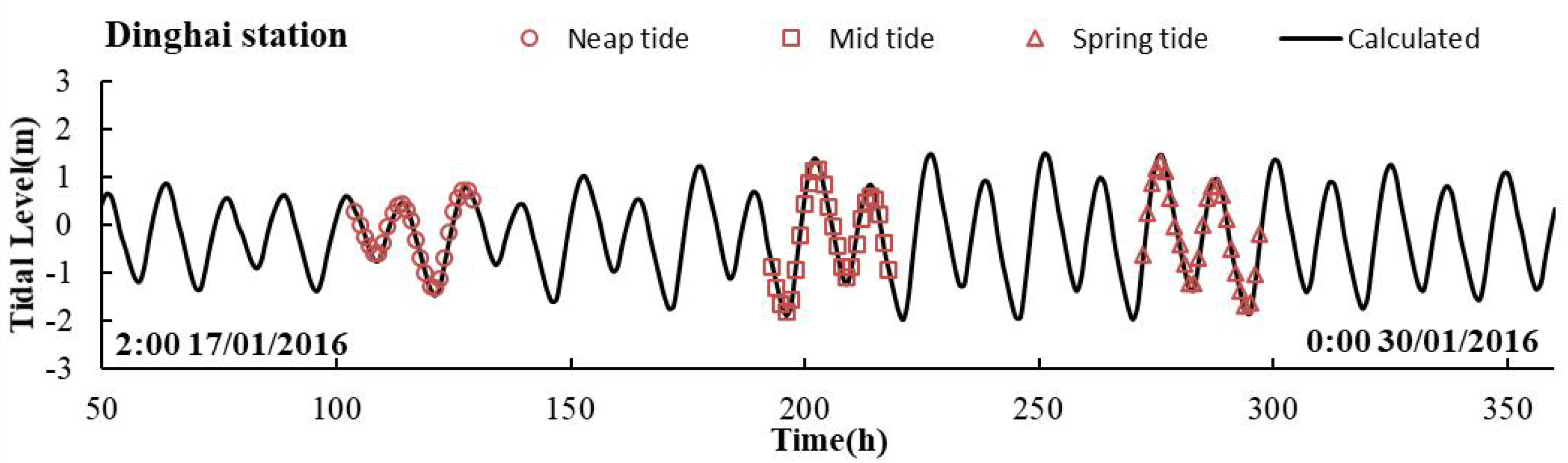
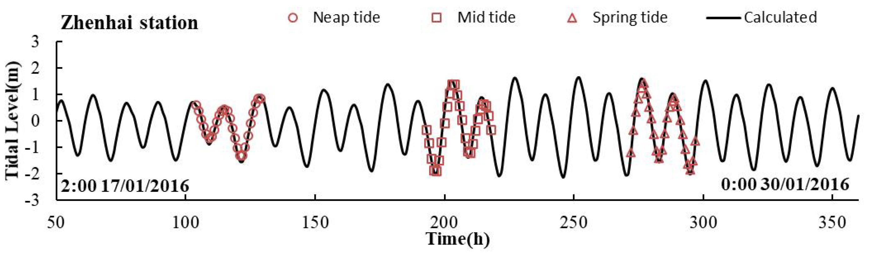
Model validation is an important step in determining the accuracy of a model, in order to conduct model experiments [31]. Actual measurement data were required to validate the water level, flow velocity, and direction of the hydrodynamic model, to ensure the accuracy of the prediction. In this study, a dataset consisting of water level, flow velocity, and direction measurements obtained in January 2016 was used to validate the model. The water level and current speed measurement stations are shown in Figure 3b. The processes of tidal level and flow velocity for spring tide, mid tide, and neap tide were used for validation. Not all of the validation procedures are listed in this paper, due to space limitations.

Figure 4 and Figure 5 show that the calculated values were in good agreement with the measured values. The correlation coefficients (R²) between the calculated and measured data at the stations, shown in

Table 2. Correlation coefficients between calculated and measured values at the tidal and current stations.

Verification Station ID	R2 of Measured vs. Calculated
	Tidal Level	Current Speed	Current Direction
Dinghai	0.984	/	/
Zhenhai	0.958	/
S1	/	0.977	0.996
S2	/	0.961	0.990
S3	/	0.961	0.984

, indicated that the results of the model were in reasonable agreement with the measured datasets.

Table 2 shows the correlation coefficients (R²) between the modeled and measured data at the water level and flow stations. The results showed reasonable agreement between the model and the measured data.

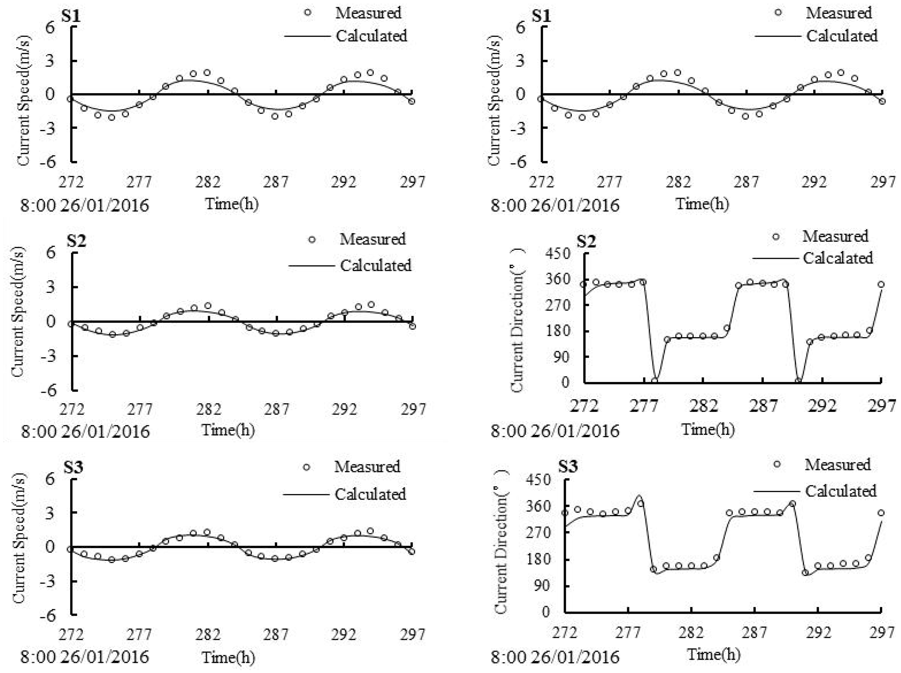
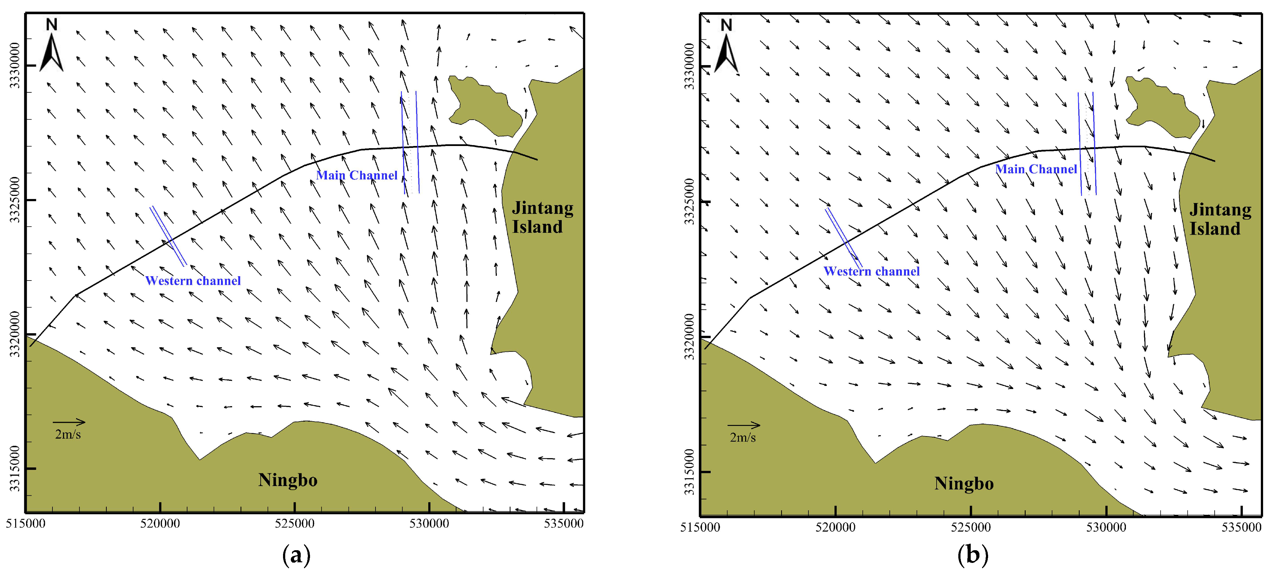
The vector diagrams of the rapid flow of the flood and ebb tides in the simulated area are shown in Figure 6. It can be seen from Figure 6 that when the tide was high, the forward tidal wave from the East China Sea passed into the calculation area from the southeast direction, the tidal wave from the middle and southern sea area entered Hangzhou Bay after passing around many islands, and the tidal wave from the northern sea area passed through the ocean near Shengshan and other sea areas, and moved towards the mouth of the Yangtze River. When the tide was low, the direction of flow was basically opposite to that of the high tide, while the path was essentially the same as that of the high tide.

The distribution pattern of the flow direction of the sea in the Jintang bridge area is not complicated: the tide rises from the southeast of the narrow mouth of the water flow to the northwest of the broad water, and vice versa for the falling tide; in addition, from near the shore of Jintang Island to the west, the flow velocity shows a gradually decreasing trend.

5. Suspended Sediment Diffusion and Transport Model

5.1. Governing Equations of the Sediment Model

Based on the validation of the hydrodynamic model and the analysis of the results, a suspended sediment dispersion and transport model was established for the simulation of the suspended sediment concentration distribution, with the following governing Equation (7):

$$\frac{\partial (hC)}{\partial t}+\frac{\partial (huC)}{\partial x}+\frac{\partial (hvC)}{\partial y}=\frac{\partial }{\partial x}\left({\epsilon }_{x}h\frac{\partial C}{\partial x}\right)+\frac{\partial }{\partial y}\left({\epsilon }_{y}h\frac{\partial C}{\partial y}\right)+F_c$$

(7)

where C is the average sediment concentration at a water depth; ε_x and ε_y are the diffusion coefficients in the x and y directions, respectively; and F_c is the source–sink term for suspended sediment flux or sediment erosion or deposition, given by the following:

$$F_c=\left\{\begin{array}{cc}\alpha \omega C({\tau }_b/{\tau }_d-1)& {\tau }_b<{\tau }_d\\ 0& {\tau }_d\le {\tau }_b\le {\tau }_e\\ M({\tau }_b/{\tau }_e-1)& {\tau }_b>{\tau }_e\end{array}\right.$$

(8)

where α is the probability of the sediment settling, varying from 0.67 to 0.84 [21]; ω is the settling velocity of the suspended sediment; M is the coefficient of scouring; τ_b is the shear stress; τ_e is the critical bed shear stress for erosion; and τ_d is the critical bed shear stress for deposition.

5.2. Validation of SSC

The SSC dataset of synchronous observations from the simulation sea area in January 2016 was used to verify the suspended sediment model; the arrangement of SSC measurement stations is shown in Figure 3b, and the corresponding verification results are shown in Figure 7. Here, only the spring tide validation results are shown. It can be seen from Figure 7 and

Table 3. Correlation coefficients between calculated and measured values at the tidal and current stations.

Verification Station ID	R2 of Measured vs. Calculated
	SSC
S1	0.658
S2	0.709
S3	0.677

that the calculated results of the sediment model were in good agreement with the measured dataset; thus, this model could be used to simulate and analyze the impact of suspended sediment generated by the construction of arresting facilities in the nearby sea area.

5.3. Construction of Suspended Sediment Source Intensity and Source Point Distribution

According to the construction characteristics of the project combined with the hydrodynamic environment characteristics of the sea, the suspended sediment generated during the construction of the arresting facilities was mainly caused by the mooring anchor placement. Since the disturbance time of the mooring anchor to the bottom bed sediment was negligible compared to the transport and diffusion time of the suspended sediment under hydrodynamic action, the source intensity of the suspended sediment generated by the mooring anchor could be approximated by instantaneous consideration. According to the consideration, dropping a single 20-ton mooring anchor would displace 8 m³ of bottom sediment, construction material, and substrate; therefore, the instantaneous source strength was determined as 1.6 m³. According to the conditions of the mooring environment, construction process, and substrate composition, the sediment suspension rate was 20%, the dry density of the sediment was 700 kg/m³, and the instantaneous source strength was 112 kg/s when the mooring anchor was placed.

The center points of each blocking unit were taken as representative points for mooring anchor placement (numbered 1#~8#), and their distribution is shown in Figure 8. The flow velocities at 1#~8# were compared and analyzed, and the comparison results are shown in

Table 4. Flow velocity at the representative position of each arresting unit during the flood and ebb of the spring tide.

Time	Western Channel (m/s)				Main Channel (m/s)
	1#	2#	3#	4#	5#	6#	7#	8#
Flood	0.82	0.93	0.99	0.88	1.09	1.28	1.35	1.04
Ebb	0.86	0.96	0.83	0.76	1.08	1.22	1.43	0.92

.

According to the comparison results, during the flood tide, the maximum velocity points of the western channel and the main channel sea area were 3# and 7#, respectively; during ebb tide, the maximum velocity points of the western channel and the main channel sea area were 2# and 7#, respectively. In order to consider the influence of suspended sediment diffusion during the worst conditions of the studied sea, four working conditions were considered: flood tide at 7# (working condition 1), ebb tide at 7# (working condition 2), flood tide at 3# (working condition 3), and ebb tide at 2# (working condition 4).

6. Results and Discussion

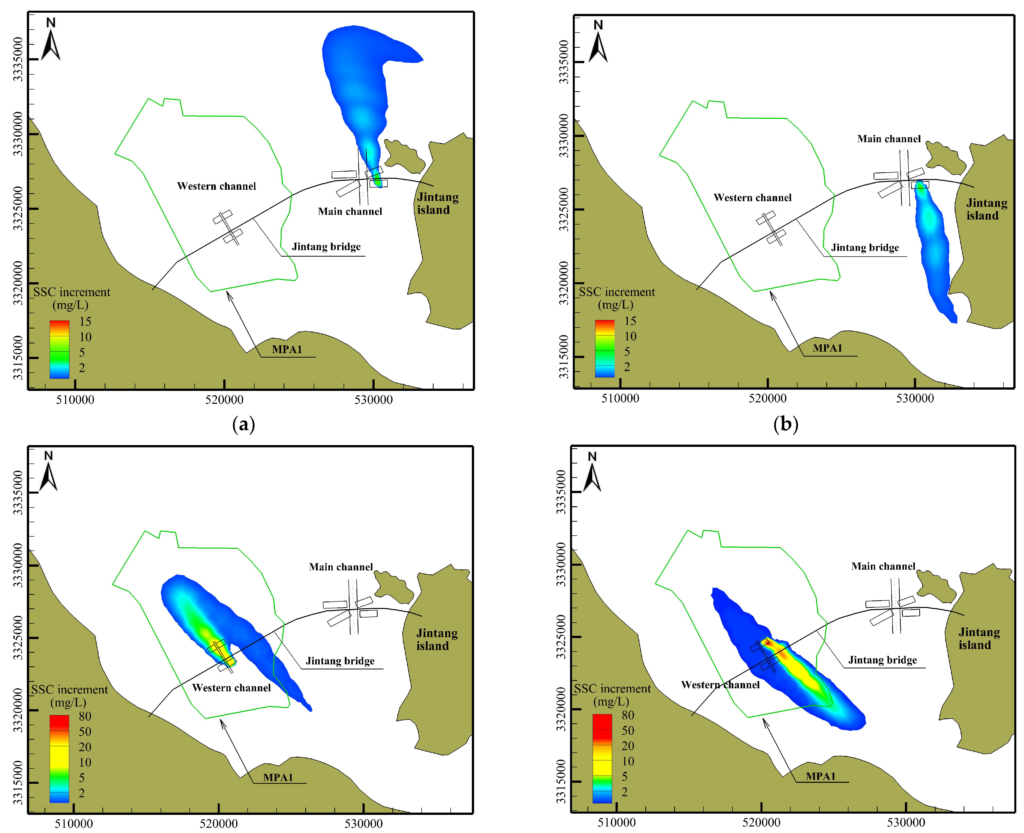
The distribution of the increase in SSC in each working condition under the combined effect of the local sand content and the source strength of the suspended sediment during the implementation of the arresting facility is shown in Figure 9, and the corresponding areas affected by the increase in SSC are shown in

Table 5. Influence area of diffused suspended sediment under different conditions.

Conditions	Area km2
	2 mg/L	5 mg/L	10 mg/L	20 mg/L	50 mg/L
Condition 1	6.127	0.166	0.081	0	0
Condition 2	3.716	0.204	0.019	0	0
Condition 3	17.198	4.381	2.199	0.484	0.031
Condition 4	14.047	5.315	3.108	1.140	0.115

.

From Figure 9 and Table 5, it can be seen that the suspended sediment mainly spread in the direction of the rising and falling tides. Due to the deeper water and the strong capacity of the holding sediment in the main channel sea, the speed of suspended sediment transport, diffusion, and dilution was faster, and compared with the western channel sea area, the scope and magnitude of the increase in SSC were smaller. Further analysis showed that when the mooring anchor near the main channel was placed during rising tide, the suspended sediment diffusion area was distributed in the sea area to the northwest of Jintang Island. During falling tide, the suspended sediment diffusion area was distributed in the local sea area to the west of Jintang Island and to the south of Jintang bridge, and its scope was obviously reduced compared with that during the rising tide. When the mooring anchor near the western channel was placed during rising or falling tide, the suspended sediment diffusion area was distributed in a band on both sides of the western channel.

It can be seen from the analysis in Table 5 that the maximum value of SSC increment in the studied sea under each working condition exceeded 10 mg/L. The seawater quality near the project area did not meet the first and second class water quality standards [32] and this had an impact on the water quality of the studied sea.

Further analysis showed that when the arresting facilities were implemented near the main channel, the area of the sea where the increase in SSC reached 10 mg/L was less than 0.1 km² and concentrated within 500 m of the arresting facilities. When the arresting facilities near the western channel were implemented during rising tide, the area of the sea where the increase in SSC reached 10 mg/L was less than 2.5 km² and the farthest point was located 4.5 km to the north of the arresting facilities; when implementation occurred during falling tide, the corresponding sea area was less than 3.5 km², and the farthest point was located 6.5 km south of the arresting facilities.

As the western channel is within MPA1, this MPA will be most affected by the suspension of sand during construction, except for other MPAs where water quality is not affected by the suspension of sediment. Our comprehensive analysis showed that the implementation of the Jintang bridge arresting facilities will have a limited impact on seawater quality.

The main objective of this study was to use pier generalization models in a hydrodynamic model [23,26,28,29], to investigate the diffusion of suspended sediment under different construction conditions. From the results of the model, it can be seen that the pier generalization methods were well applied and saved time and costs during model calculations. Among the four working conditions, working conditions 2 and 3 were blocked by Jintang Island, and the diffusion of sediment suspended during construction was smaller than in working conditions 1 and 2. The spread of suspended sediment was the widest in condition 3 (2 mg/L), while the impact range of suspended sediment (greater than 2 mg/L) was smaller than that of condition 4. All four conditions showed the impact range of suspended sediment spread under the most unfavorable conditions, and these unfavorable conditions were avoided in the specific construction.

7. Conclusions

In this paper, taking the Jintang bridge as an example and using the equivalent roughness method to generalize the bridge piers, a 2D hydrodynamic and sediment numerical model was applied to simulate the distribution of suspended sediment dispersion and transport caused by the implementation of non-navigable channel arresting facilities. In addition, the environmental impact on water quality was analyzed, and the following conclusions were obtained.

The new formula for equivalent roughness used in this paper is applicable to near-shore waters, with its simple structure, comprehensive consideration, and easy application; it can be used to obtain reasonable simulation results in waters of interest.

When the arresting facilities were implemented, the suspended sediment mainly spread along the main flow of high and low tide. When implemented near the main channel, the sea area where the increase in SSC reached 10 mg/L was concentrated within 500 m of the arresting facility; when implemented near the western channel, the corresponding sea area was concentrated within the range of 4.5 km north to 6.5 km south of the arresting facility. In general, the impact of the implementation of the arresting facilities on seawater quality was relatively limited.

The implementation of the arresting facilities affected the water quality of MPA1, as shown by an increase in suspended sediment; the other MPAs were not affected by the increase in suspended sediment from construction.

One limitation of this study is that only the dynamics of tidal currents were considered, while the dynamic factor of waves was not taken into account, which would have mad the spread of the suspended sediment simulation small. In future research, new methods for suspended sediment simulation should be considered, and the effect of coupling wave and tidal currents on the diffusion of suspended sediment, as well as the effect of different construction processes on the diffusion of suspended sediment, should also be investigated.

References

- Ren, H.; Wang, Y.; Xiao, G.; Yan, X.F. Active early-warning system for bridge piers against ship collision and its expriement. Laser Infrared 2013, 43, 66–70. [Google Scholar]
- Chen, M.D.; Xiang, Y. A study of combined anti-collision scheme for protection of non-navigable piers. Hydro-Sci. Eng. 2014, 4, 98–104. [Google Scholar]
- Wang, B.K.; Yang, T.; Yang, L.M.; Liu, J.; Tong, X.L.; Zhou, F.H.; Wang, Y.G. Impact tests and hydrodynamic analysis of an adaptive arresting net crashworthy device for protecting piers against ship collisions. Ocean Eng. 2017, 35, 90–96. [Google Scholar]
- Yao, S.S.; Xie, M.X.; Zhao, H.B. Numerical simulation study on impacts of suspended sediment diffusion on water intaking during construction period for power plant project. J. Waterw. Harb. 2014, 35, 118–124. [Google Scholar]
- Erftemeijer, P.L.A.; Robin Lewis, R.R. Environmental impacts of dredging on seagrasses: A review. Mar. Pollut. Bull. 2006, 52, 1553–1572. [Google Scholar] [CrossRef] [PubMed]
- Yang, S.L.; Zhang, J.; Xu, X.J. Influence of the Three Gorges Dam on downstream delivery of sediment and its environmental implications, Yangtze River. Geophys. Res. Lett. 2007, 34, GL029472. [Google Scholar] [CrossRef]
- Bray, R.N. Environmental Aspects of Dredging; CRC Press: Boca Raton, FL, USA, 2008. [Google Scholar]
- Nielsen, M.H.; Bach, L.; Bollwerk, S.M. Spreading of sediment due to underwater blasting and dredging: Field observations from quay construction in Sisimiut, Greenland. Ocean Coast. Manag. 2015, 116, 512–522. [Google Scholar] [CrossRef]
- Manap, N.; Voulvoulis, N. Data analysis for environmental impact of dredging. J. Clean. Prod. 2016, 137, 394–404. [Google Scholar] [CrossRef]
- Bach, L.; Nielsen, M.H.; Bollwerk, S.M. Environmental Impact of Submarine Rock Blasting and Dredging Operations in an Arctic Harbor Area: Dispersal and Bioavailability of Sediment-Associated Heavy Metals. Water Air Soil Pollut. 2017, 228, 198. [Google Scholar] [CrossRef]
- Bianchini, A.; Cento, F.; Guzzini, A.; Pellegrini, M.; Saccani, C. Sediment management in coastal infrastructures: Techno-economic and environmental impact assessment of alternative technologies to dredging. J. Environ. Manag. 2019, 248, 109332. [Google Scholar] [CrossRef]
- Svensson, N.; Norén, A.; Modin, O.; Karlfeldt Fedje, K.; Rauch, S.; Strömvall, A.-M.; Andersson-Sköld, Y. Integrated cost and environmental impact assessment of management options for dredged sediment. Waste Manag. 2022, 138, 30–40. [Google Scholar] [CrossRef] [PubMed]
- Juez, C.; Battisacco, E.; Schleiss, A.J.; Franca, M.J. Assessment of the performance of numerical modeling in reproducing a replenishment of sediments in a water-worked channel. Adv. Water Resour. 2016, 92, 10–22. [Google Scholar] [CrossRef]
- Yan, K.; Liang, Q.X. Coastal Engineering; China Ocean Press: Nanjing, China, 2002. [Google Scholar]
- Smagorinsky, J. General circulation experiments with the primitive equations: I. The basic experiment. Mon. Weather Rev. 1963, 91, 99–164. [Google Scholar] [CrossRef]
- Anastasiou, K.; Chan, C.T. Solution of the 2D shallow water equations using the finite volume method on unstructured triangular meshes. Int. J. Numer. Methods Fluids 1997, 24, 1225–1245. [Google Scholar] [CrossRef]
- Jiwen, W.; Ruxun, L. The composite finite volume method on unstructured meshes for the two-dimensional shallow water equations. Int. J. Numer. Methods Fluids 2001, 37, 933–949. [Google Scholar] [CrossRef]
- Choi, B.J.; Iskandarani, M.; Levin, J.; Haidvogel, D.B. A spectral finite-volume method for the shallow water equations. Mon. Weather Rev. 2004, 132, 1777–1791. [Google Scholar] [CrossRef] [Green Version]
- Zhao, D.; Shen, H.; Tabios, G., III; Lai, J.; Tan, W. Finite-volume two-dimensional unsteady-flow model for river basins. J. Hydraul. Eng. 1994, 120, 863–883. [Google Scholar] [CrossRef]
- Sleigh, P.; Gaskell, P.; Berzins, M.; Wright, N. An unstructured finite-volume algorithm for predicting flow in rivers and estuaries. Comput. Fluids 1998, 27, 479–508. [Google Scholar] [CrossRef]
- Li, Y.; Song, Z.; Peng, G.; Fang, X.; Li, R.; Chen, P.; Hong, H. Modeling Hydro-Dynamics in a Harbor Area in the Daishan Island, China. Water 2019, 11, 192. [Google Scholar] [CrossRef] [Green Version]
- Padman, L.; Erofeeva, S. Tide Model Driver (TMD) Manual. Earth & Space Research; The MathWorks: Natick, MA, USA, 2005. [Google Scholar]
- Van Rijn, L.C. Equivalent Roughness of Alluvial Bed. J. Hydraul. Div. 1982, 108, 1215–1218. [Google Scholar] [CrossRef]
- Chang, W.-Y.; Constantinescu, G.; Lien, H.-C.; Tsai, W.-F.; Lai, J.-S.; Loh, C.-H. Flow Structure around Bridge Piers of Varying Geometrical Complexity. J. Hydraul. Eng. 2013, 139, 812–826. [Google Scholar] [CrossRef]
- Amini, A.; Parto, A.A. 3D numerical simulation of flow field around twin piles. Acta Geophys. 2017, 65, 1243–1251. [Google Scholar] [CrossRef]
- Fael, C.; Lança, R.; Cardoso, A. Effect of pier shape and pier alignment on the equilibrium scour depth at single piers. Int. J. Sediment Res. 2016, 31, 244–250. [Google Scholar] [CrossRef]
- Ben Mohammad Khajeh, S.; Vaghefi, M.; Mahmoudi, A. The scour pattern around an inclined cylindrical pier in a sharp 180-degree bend: An experimental study. Int. J. River Basin Manag. 2017, 15, 207–218. [Google Scholar] [CrossRef]
- Yang, X.; Qian, J.; Weng, S. Determination of Equivalent Roughness of Bridge Piers’ Flow Resistance. J. Hydrol. Eng. 2019, 24, 04019024. [Google Scholar] [CrossRef]
- Zu, X.H.; Li, R.J.; Dai, L.; Li, Y.T. Equivalent roughness of pier under unsteady flow. J. Waterw. Harb. 2016, 37, 514–519. [Google Scholar]
- Li, R.J.; Zheng, J.; Feng, Q.; Zhang, W.H. Sediment carrying capacity and erosion rate of nearshore sediment. J. Sediment Res. 2013, 37, 21–25. [Google Scholar]
- Pinto, L.; Fortunato, A.; Zhang, Y.; Oliveira, A.; Sancho, F. Development and validation of a three-dimensional morphodynamic modelling system for non-cohesive sediments. Ocean Model. 2012, 57, 1–14. [Google Scholar] [CrossRef]
- Ministry of Ecology and Environment of the People’s Republic of China. Sea Water Quality Standard; Ministry of Ecology and Environment of the People’s Republic of China: Beijing, China, 1998; pp. 15–21. [Google Scholar]
Figure 1.
Location of the Jintang bridge and the layout of the arresting facilities. (a) Scheme of arresting facilities; (b) arresting facilities site layout.
Figure 2.
Flowchart map.
Figure 3.
Study area used in the investigation: (a) mesh generation and relief map of simulation area; (b) layout of the observation stations.
Figure 4.
Verification of the tidal level at Dinghai and Zhenhai stations.
Figure 5.
Verification of the current speed and direction during spring tide at station S1, S2, and S3.
Figure 6.
Rapid flow chart of tidal fluctuation: (a) flood tide, and (b) ebb tide.
Figure 7.
Verification of SSC during the spring tide at stations S1, S2, and S3.
Figure 8.
Layout of the representative mooring anchor of each arresting unit.
Figure 9.
Distribution of the increase in suspended sediment concentration under all four conditions: (a) condition 1; (b) condition 2; (c) condition 3; and (d) condition 4.