

Surface Feature Prediction for Laser Ablated 40Cr13 Stainless Steel Based on Extreme Learning Machine

1
School of Mechanical Engineering and Automation, Beihang University, Beijing 100191, China
2
Jiangxi Research Institute, Beihang University, Nanchang 330096, China
3
Research and Application Center of Advanced CNC Machining Technology, Beijing 100191, China
4
Research Center of High-Efficient and Green CNC Machining Process and Equipment, Beijing 100191, China
*
Author to whom correspondence should be addressed.
Materials 2023, 16(2), 505; https://doi.org/10.3390/ma16020505
Submission received: 19 November 2022
/
Revised: 22 December 2022
/
Accepted: 3 January 2023
/
Published: 4 January 2023
(This article belongs to the Special Issue Advanced Laser Microfabrication)
Abstract
:Determining an optimal combination of laser process parameters can significantly improve the efficiency and quality of 40Cr13 steel surface processing. In this study, two machine learning models (ELMSS and ELMPS) were proposed to predict the processing results of surface features to optimize process parameters. The prediction accuracies of the proposed models were always higher than those of traditional back propagation (BP) and radial basis function (RBF) neural networks, and the calculation time of the proposed models was significantly reduced. In comparison, the prediction accuracy ranking for ablation depth was ELMSS (92.6%), BP (89.8%), and RBF (89.6%), and for the ablation width, it was ELMSS (98.3%), BP (97.4%), and RBF (96.1%). The material removal rate was 92.4%, 91.1%, and 89.1% for ELMSS, BP, and RBF, respectively. Finally, the prediction accuracy ranking for surface roughness was 86.8%, 80.7%, and 79.5% for ELMPS, BP, and RBF, respectively. After optimization by the genetic algorithm, the prediction accuracies of the proposed models for the depth, width, material removal rate, and surface roughness reached 94.0%, 99.0%, 93.2%, and 91.2%, respectively. With the support of ELMSS and ELMPS, the results of the surface features can be predicted before machining and the appropriate process parameters can be selected in advance.
1. Introduction
Microstructures on the surface of 40Cr13 are widely used in the die industry owing to their properties, such as being aesthetically appealing, tribological, and easy to detach from injection points [1,2]. However, it is difficult to precisely process the ideal microstructure on the surface of 40Cr13 because of its hardness and strength. Laser ablation is a non-contact processing method that uses a focused spot of high energy density to instantly vaporize surface materials and is becoming an effective means of processing surface microstructures on hard-to-machine material [3,4]. The processing quality of laser ablation depends on the selection of process parameters, such as laser power, pulse frequency, and scanning speed [5]. Based on theoretical analysis and experimental results, choosing the right combination of process parameters can significantly improve the quality of laser ablation [6]. However, owing to the numerous combinations of process parameters in the laser ablation process, optimizing the process parameters through a trial-and-error approach can be time consuming. Therefore, finding a suitable method of improving optimal laser processing parameter selection to ultimately achieve precision laser ablation has become an urgent issue.
Machine learning has developed rapidly since it was proposed and has been successfully applied in the prediction of laser processing results [7]. Chen et al. [8] proposed a supervised machine learning approach to detect trajectory defects in selective laser melting, four metrics were taken as input variables to the model to quantitatively assess the quality of the trajectory. They believe that the machine learning model can significantly improve the search efficiency of process parameter windows and has great application potential in future unmanned factories. Yousef et al. [9] proposed a neural network that can be used to model a nonlinear laser micromachining process, which can help to predict the pulse energy level required to produce microstructures with the desired depth and diameter. Teixidor et al. [10] used three types of machine learning models to predict the process results of surface features. The inputs of these models are the scan speed, pulse intensity, and pulse frequency while the outputs are depth, width, surface roughness, and material removal rate (MRR). Jimin et al. [11] used a multi-layer neural network to predict the processing results of laser cutting. The inputs of the model included not only the typical parameters but also the slant angle of the laser head. Further, they applied the radial basis function (RBF) neural network to predict the processing results of stainless-steel sheets [12]. Dhupal et al. [13] applied artificial neural network (ANN) and response surface methodology to optimize the machining features of the pulsed Nd:YAG laser for microgrooving on aluminum titanate. The experimental results show that the prediction results of the two methods are consistent. Later, the genetic algorithm was applied to further adjust the model, which improved the prediction accuracy [14]. However, the calculation time of the algorithm was inevitably increased. Ciurana et al. [15] applied the ANN for predicting the quality of 3D geometrical features on AISI H13 steel and used the particle swarm optimization algorithm to improve the accuracy. The back propagation (BP) neural network, which is another typical prediction model, was successfully applied to optimize the process parameters of laser micro-machining [16,17].
Despite the successful application of the above machine learning models to the prediction of laser ablation surface features, a few limitations still exist. First, the above-mentioned models require a large amount of experimental data for training to achieve high prediction accuracy. In addition, the computational efficiency of these algorithms is relatively low and the training time of the models is on the second level, making them unsuitable for real-time applications.
The technological test of laser ablated 40Cr13 surfaces is typically time-consuming and laborious, and it is difficult to obtain a large amount of data to train a prediction model. Therefore, an accurate and efficient method that can be used to predict surface features with limited experimental data is required. To the best of our knowledge, there are only a few scientific studies on the laser ablation of 40Cr13 to obtain target surface features. Our objective is to bridge this knowledge gap and improve the laser ablation quality of superhard materials such as 40Cr13 stainless steel.
This paper presents an extreme learning machine of single-track scanning (ELMSS) and plane scanning (ELMPS) for the prediction of the surface features, which improve prediction accuracies and significantly reduce the training time.
The novelties of this study are that the extreme learning machine is applied to the prediction of the laser processing surface features for the first time, all the unknown parameters in the ELMSS and ELMPS are determined, and the accurate prediction of the surface feature of nanosecond laser processing 40Cr13 material is realized. The practical significance of the presented methodology is that researchers can use the proposed models to accurately predict the dimension of surface features according to the input laser processing process parameters. If the dimension cannot meet the tolerance requirements, the process parameters must be modified. In this way, In this way, trial and error experiments do not need to be conducted, which reduces the time and labor costs.
The rest of this paper is organized as follows: Section 2 introduces the experimental details. Section 3 presents the establishment of the prediction models. Section 4 compares the prediction accuracies and algorithm efficiency of presented models and those of two other ANN models. Section 5 utilizes the genetic algorithm to further improve the prediction accuracies of ELMSS and ELMPS. Finally, Section 6 presents the concluding remarks of the study.
2. Experiment Details
2.1. Material
40Cr13 stainless steel was used in this study, and its main components are listed in Table 1. The chemical composition analysis was conducted by suppliers (Yuzhixiang Material Co., Suzhou, China). 40Cr13 has high hardness, abrasion resistance, and corrosion resistance and is widely used to manufacture high-end precision molds. The surfaces of the samples were milled and ground before the technological tests to eliminate potential influences of the initial surface roughness on the machining results [17].
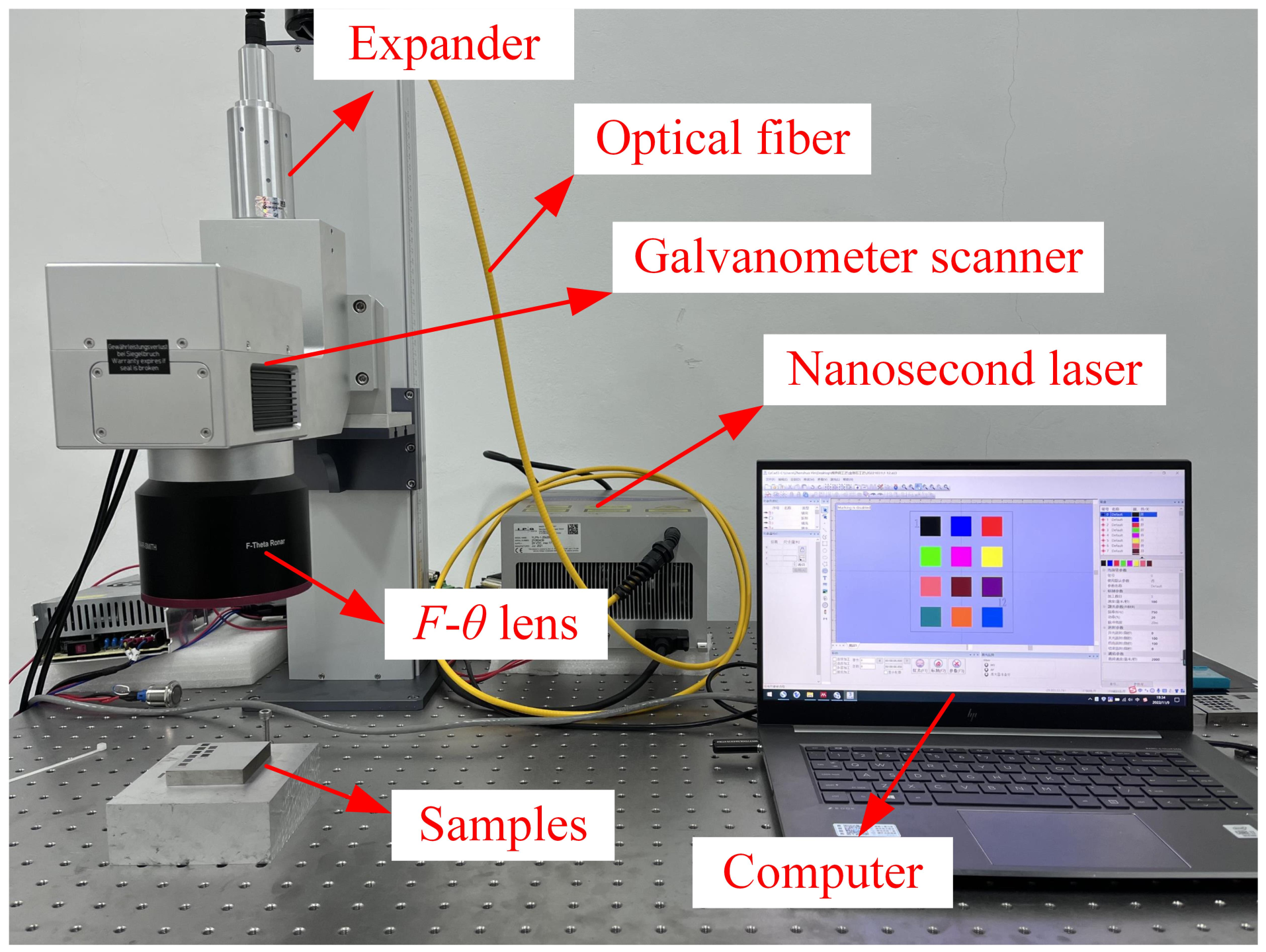
2.2. Experimental Platform
The experimental platform is shown in Figure 1. This study used a nanosecond pulse laser generator (FORMULA-355, Advanced Optowave Co., New York, NY, USA) with a wavelength of 355 nm, and its main parameters are listed in Table 2. The output spot of the laser generator enters a 3D galvanometer scanner (G3-3D, JCZ Technology Co., Beijing, China) with a focal length of 290 mm through a beam expander (BEX-355-6X, Wavelength OE Co., Nanjing, China) and uses an F-theta field lens (SL-355, Wavelength OE Co., Nanjing, China) to focus the laser spot on the surface of the samples. The diameter of focus spot is 19.38 μm. The laser power irradiating on the surfaces was measured with a power meter (Ophir 30A-SV-17, Thorlabs Co., Newton, MA, USA) [17].
2.3. Technological Test Methods
To obtain excellent properties, micro-grooves and planes are taken as the two typical microstructures on the surface of the dies. These two structures are usually obtained by single-track and plane scanning, respectively. The details of these methods are given below.
2.3.1. Single-Track Scanning
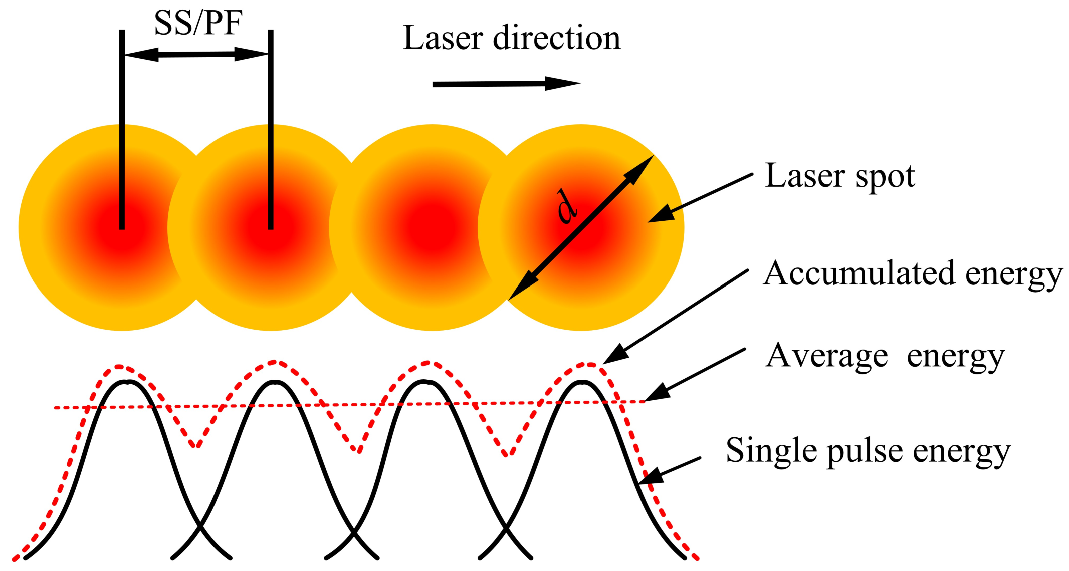
Single-track scanning is realized to ensure that the laser spot linearly scans the surface of a sample, producing a micro-groove structure by laser ablation. Its process parameters include laser power (LP), pulse frequency (PF), and scanning speed (SS). The laser pulse accumulation of single-pass machining is shown in Figure 2. Since the output power of a laser with a wavelength of 355 nm is significantly affected by the variation of the PF, the selection of the variation range of the process parameters must be reasonable. The process parameters of single-track scanning in this study are listed in Table 3. The value of a single process parameter is changed each time during processing, and other parameters remain unchanged. A total of 48 micro-grooves are processed [17].
2.3.2. Plane Scanning
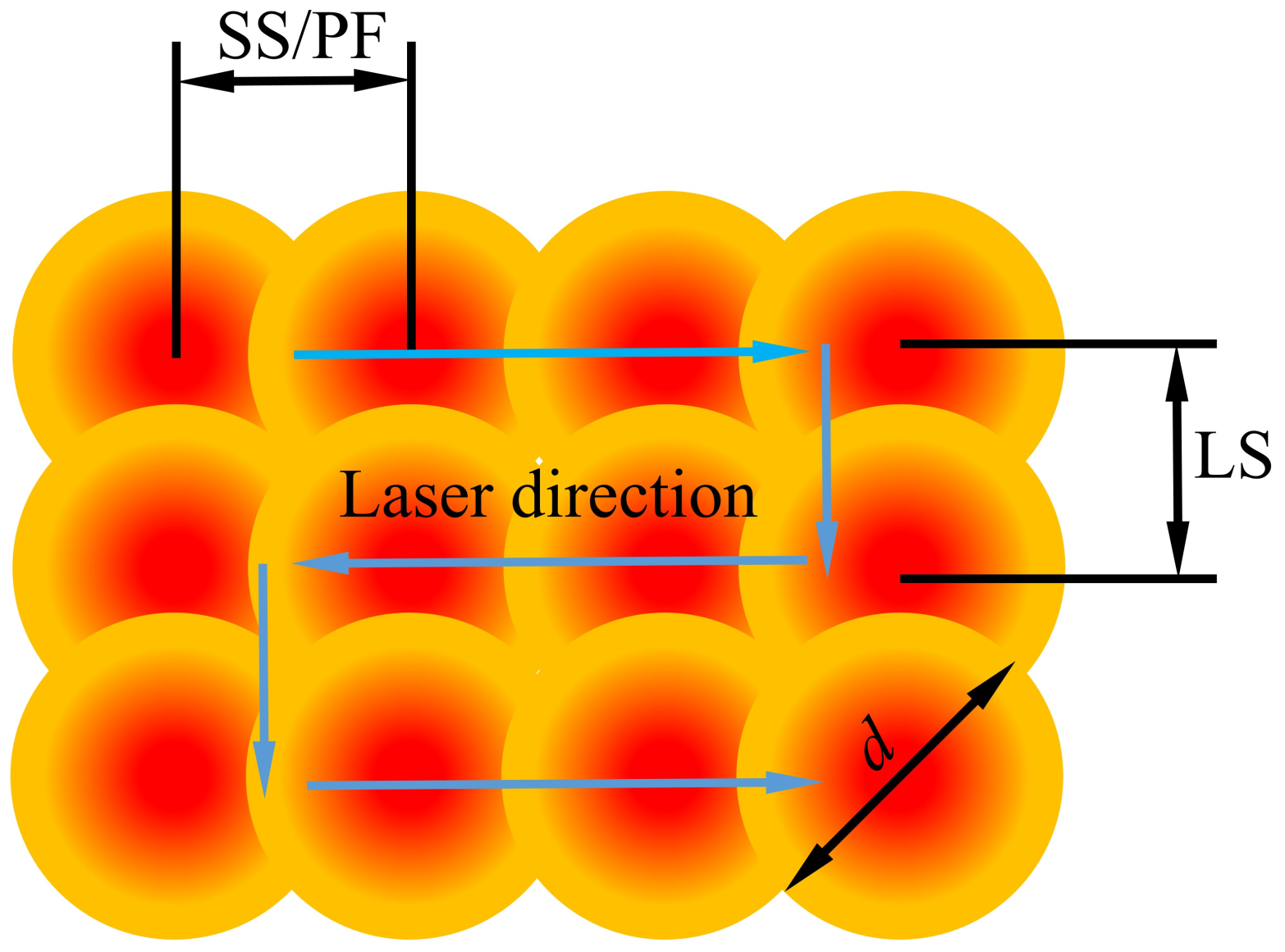
Plane scanning is realized using the laser spot for reciprocating the scanning motion on the surface of a sample with a certain line spacing (LS). Its process parameters add the LS based on single-track scanning parameters. The laser pulse accumulation of plane scanning is shown in Figure 3. The variation range of the process parameters is listed in Table 4. Similarly, the value of a single process parameter is changed during each processing while others remain fixed. A total of 81 planes are formed.
2.4. Features Measurement
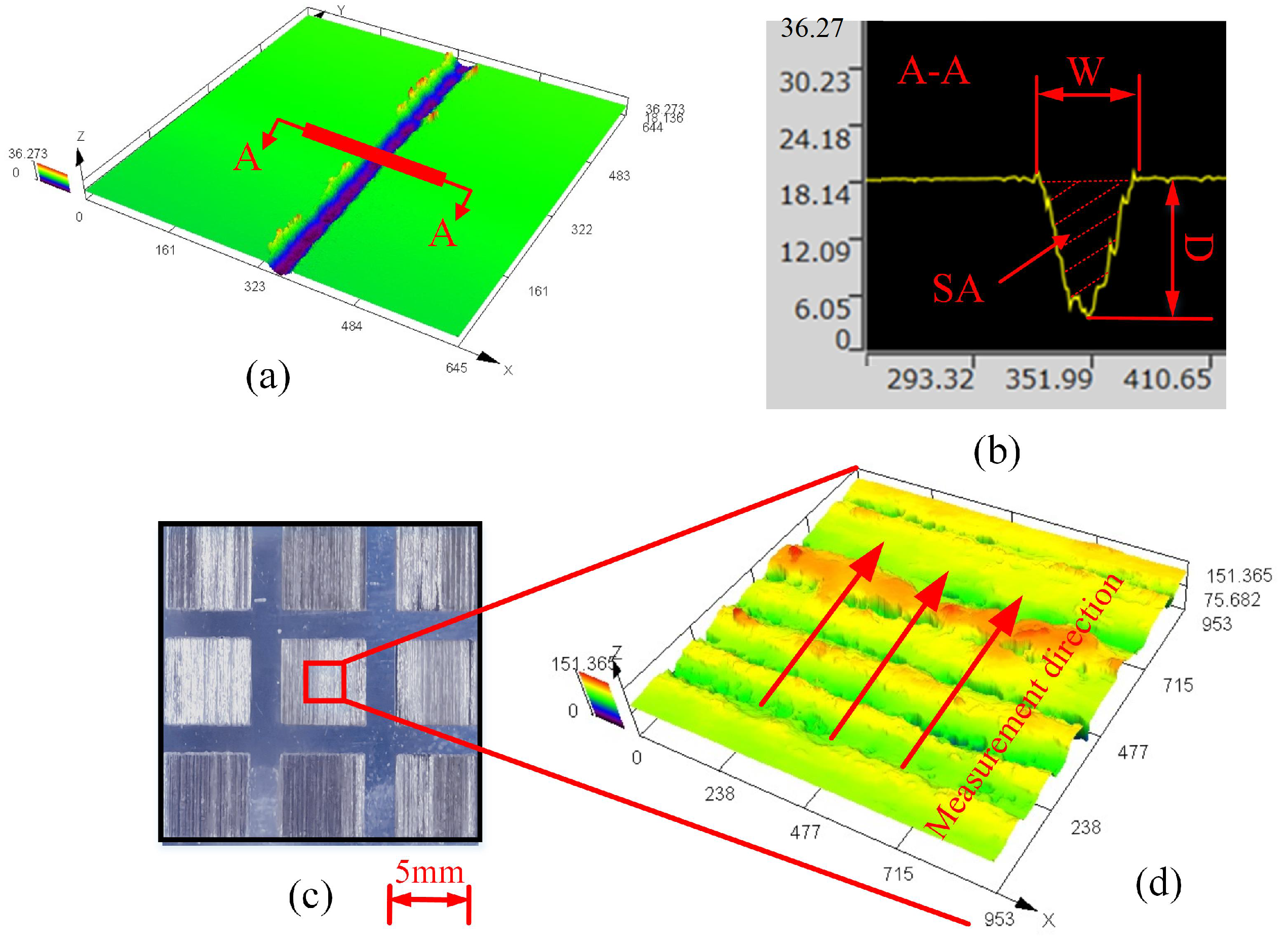
The cross-section of the microgroove structure produced by single-track laser ablation is approximately V-shaped owing to the Gaussian distribution of the laser beam [18]. The micro-groove of single-track scanning was measured by laser confocal microscopy (LEXT OLS5100, Olympus Co., Tokyo, Japan), and a typical micro-groove is shown in Figure 4a where the cross-section of the micro-groove is observed along the A-A direction. As is shown in Figure 4b, three features are defined on the cross-section: depth (D), width (W), and sectional area (SA). The material removal rate (MRR) is defined as
where SA denotes the sectional area of the micro-groove, SS denotes the scanning speed, and t denotes the scanning time.
During the measurement of D, W, and MRR, three sections with a length of 1 mm were cut along each micro-groove, and the average value was taken as the measurement result of the three features.
The physical image of the surface obtained from the plane scanning is shown in Figure 4c, and a typical surface morphology observed using LEXT OLS5100 is exemplified in Figure 4d. A contact roughness meter (SJ-310, Mitutoyo Co., Kawasaki, Japan) was used to measure the surface roughness (Ra) along the direction shown in Figure 4d. Ra was calculated as the average value of three measurements.
Measurement results of the four surface features—D, W, MRR, and Ra—obtained using the above mentioned methods are shown in Table A1 of Appendix A, which contains 48 samples of single-track scanning and 81 samples of plane scanning.
3. Establishment of the Prediction Model
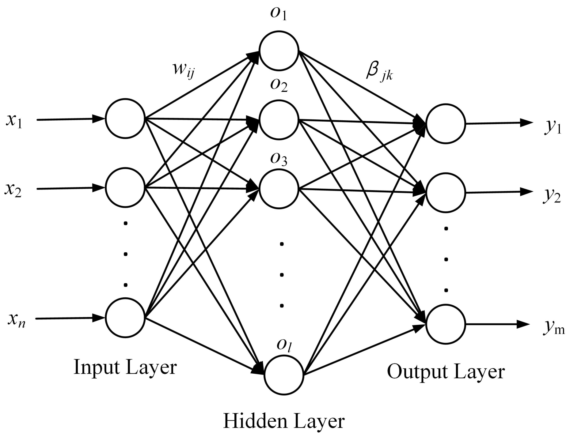
ELM was proposed by Guang-Bin Huang et al. [19] in 2004 and was soon applied to function fitting and classification problems [20,21,22]. It is part of a single-hidden-layer feedforward neural network. A typical structure of ELM is shown in Figure 5, consisting of input, hidden, and output layers. Assuming that were the neuron numbers of the input, hidden, and output layers, respectively, the connection weight matrix between the input and hidden layers is
where w represents the connection weight between the i neuron in the input layer and j neuron in the hidden layer.
The connection threshold matrix of the hidden layer is
where b represents the connection threshold of the i neuron in the hidden layer.
The connection weight matrix between the hidden and output layers is
where represents the connection weight between the j neuron in the hidden layer and k neuron in the output layer.
Assuming that there are P samples in the training set data, the input and output matrices of ELM can be expressed, respectively, as
If g(x) denotes the activation function, the output matrix of the hidden layer then becomes
Guang-Bin Huang et al. [19] pointed out that, when the activation function g(x) is infinitely differentiable, the connection weight between the hidden and output layers can be obtained using:
where H is the Moore–Penrose inverse of the hidden layer output matrix.
The connection weight (W) and threshold (b) between the input and hidden layers can be randomly generated before training and remain unchanged during the training process. After the activation function g(x) is determined before training and the connection weight () is solved using Equation (8), all the parameters of ELM are determined. The entire training process does not require error back-propagation and iterative calculation. Hence, the training time of ELM can be greatly reduced on the premise of ensuring prediction accuracy.
Assuming that there are Q samples in the test set data, the prediction result of ELM is:
where w and b are the preset connection weights and thresholds, respectively, is the calculation result of training, and x is the input data of the test set.
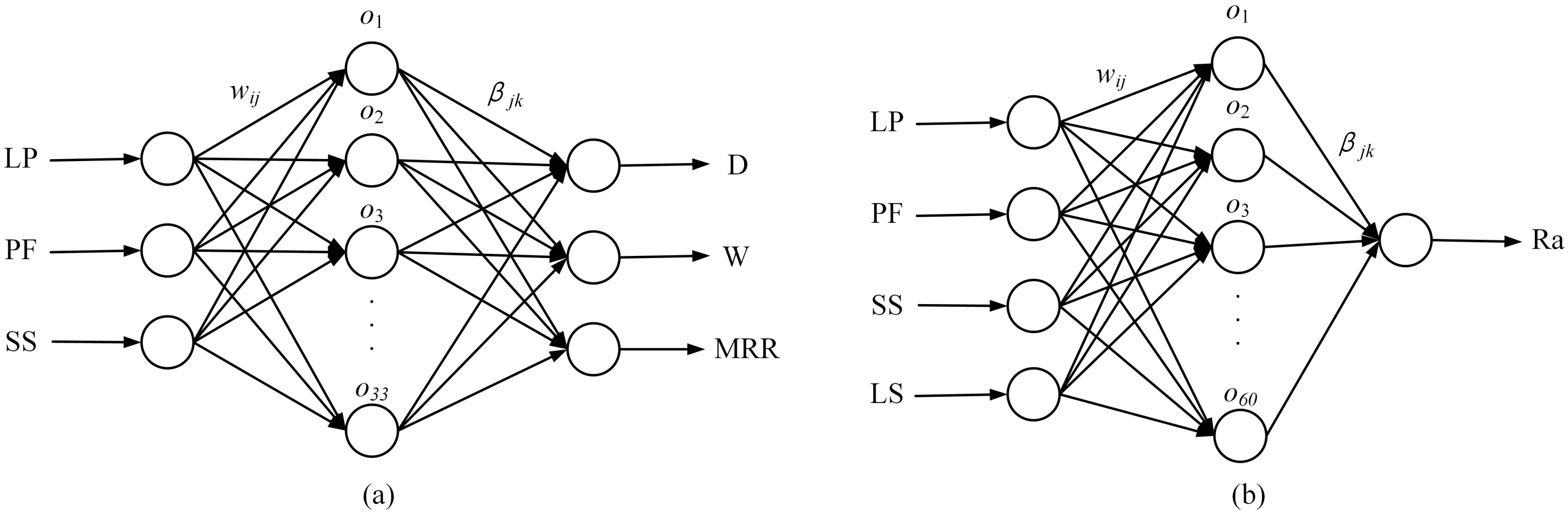
The ELM model for predicting the surface features was developed using MATLAB R2018a software. The single-track scanning (ELMSS) model proposed for feature prediction is shown in Figure 6a. LP, PF, and SS were set as the input layer parameters, and D, W, and MRR as the output layer parameters. The number of neurons in the hidden layer was 33, and the activation function was “sigmoid.” The plane scanning (ELMPS) model is shown in Figure 6b. LS was added to the input layer parameters, and the output layer parameter was changed to Ra. The number of neurons in the hidden layer was 60, and the activation function was again “sigmoid”.
Groups 1–45 of data in Table A1 of Appendix A were treated as the training set and groups 46–48 as the test set. Based on the ELM model, the surface features were predicted through the following process.
First, the technological test was carried out according to the designed parameters, and the machining result data of the surface features were obtained.
Second, the data were categorized into training and test sets after they were normalized, and the number of neurons in the hidden layer was determined. The connection weights (W) and thresholds (b) between the input layer and the hidden layer were randomly set.
Third, an infinitely differentiable activation function was selected, and the hidden layer output matrix (H) combining the data of the training sets was calculated.
Fourth, the connection weights () between the hidden and output layers were calculated to complete the training of the ELM model.
Finally, the test set data were inputted into the trained model, the predicted results were compared with the measured results, and the prediction accuracy of the ELMSS and ELMPS was analyzed.
The ELMSS and ELMPS are based on a typical perceptron with one hidden layer. The innovation of this paper is to find the most suitable number of neurons in the hidden layer used to predict the surface feature of laser processing and use the genetic algorithm to optimize the connection weight and threshold to obtain the highest prediction accuracy.
4. Prediction Results of ELMSS and ELMPS
To verify the accuracy of the ELMSS, the prediction results were compared with that of BP [16] and RBF [12] neural network machine learning models for the same training and test data sets. For the prediction models of single-track scanning, the network structure of the BP neural network is 3-6-3, which is the network structure with the highest prediction accuracy. The activation function of BP neural network is “tansig,” which is infinitely differentiable. The expression of the function is:
The spread value of the RBF neural network is set to 1.0. The measured values and predicted results of D, W, and MRR after training with the same data are shown in Table 5.
The average prediction accuracy is defined as
From the calculation for prediction accuracy, ELMSS has the highest accuracy for D, reaching 92.6%, followed by that of the BP and RBF neural networks, which are 89.8% and 89.6%, respectively. The prediction accuracies of the three models for W are relatively high. Among them, the ELMSS has the highest prediction accuracy of 98.3%, followed by the BP and RBF neural networks, with prediction accuracies of 97.4% and 96.1%, respectively. The prediction accuracy ranking for MRR is ELMSS (92.4%), BP neural network (91.1%), and RBF neural network (89.1%), respectively.
Similarly, to verify the accuracy of the ELMPS, the prediction results were compared with two other models, the network structure of the BP neural network is 4-3-1, the activation function is “tansig,” and the spread value of the RBF is still set to 1.0. The measured values and prediction results of Ra by the three models are shown in Table 6.
The average prediction accuracy of plane scanning Ra was also calculated. The average prediction accuracies of the three models for Ra were relatively low. ELMPS had the highest average accuracy of 86.8%, and the average prediction accuracies of the BP and RBF neural networks were 80.7% and 79.5%, respectively.
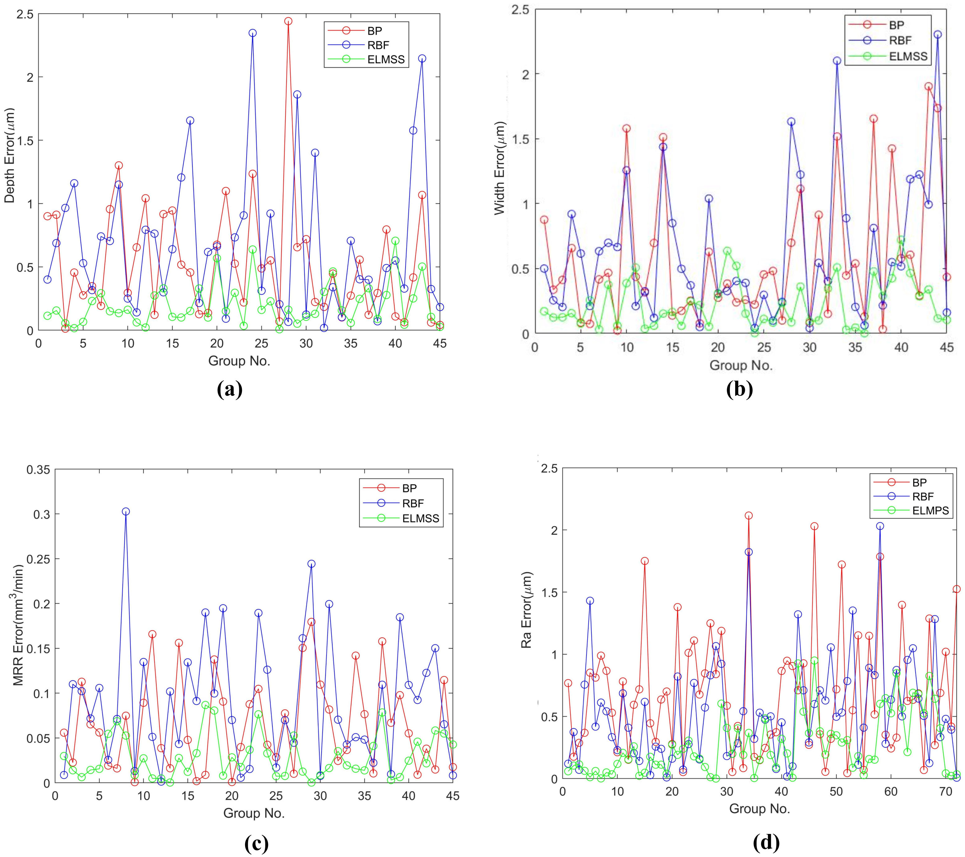
To test the generalization performance of ELMSS and ELMPS, 45 samples of the training set data in single-track scanning were treated as the input of the models, and 45 predicted values of D, W, and MRR were obtained. Further, the absolute error between the predicted and actual values was plotted in Figure 7a–c. Then, 72 samples of the training set data in plane scanning were used as the input of the models, and 72 predicted values of Ra were obtained. The absolute error between the predicted and actual values is plotted in Figure 7d. Figure 7 shows that the absolute error of ELMSS and ELMPS is minimal compared to the other two models.
The training period of the models were used to compare the computing efficiency of the three models. The CPU performance of the computing platform was unified as Intel(R) Core(TM) i7-10750H CPU @ 2.60GHz. The values of the training time are listed in Table 7. The BP neural network requires the longest calculation time, because the training process of the model needs error back propagation and iteration. The RBF neural network belongs to the forward network, but the calculation time is longer than that of ELMSS and ELMPS. In summary, the computational efficiency of the prediction models proposed in this study have been improved from tens to hundreds of times compared with the other two types of machine learning models, providing the possibility of using the ELMSS and ELMPS in real-time applications.
5. Optimization of ELMSS and ELMPS Based on Genetic Algorithm
The connection weights and thresholds from the input layer to the hidden layer of the ELMSS and ELMPS models are randomly determined, which leads to unstable prediction results. This section applied genetic algorithm to optimize the parameters of prediction models, in order to obtain the optimal connection weights and thresholds, thereby improving the prediction accuracy of the models.
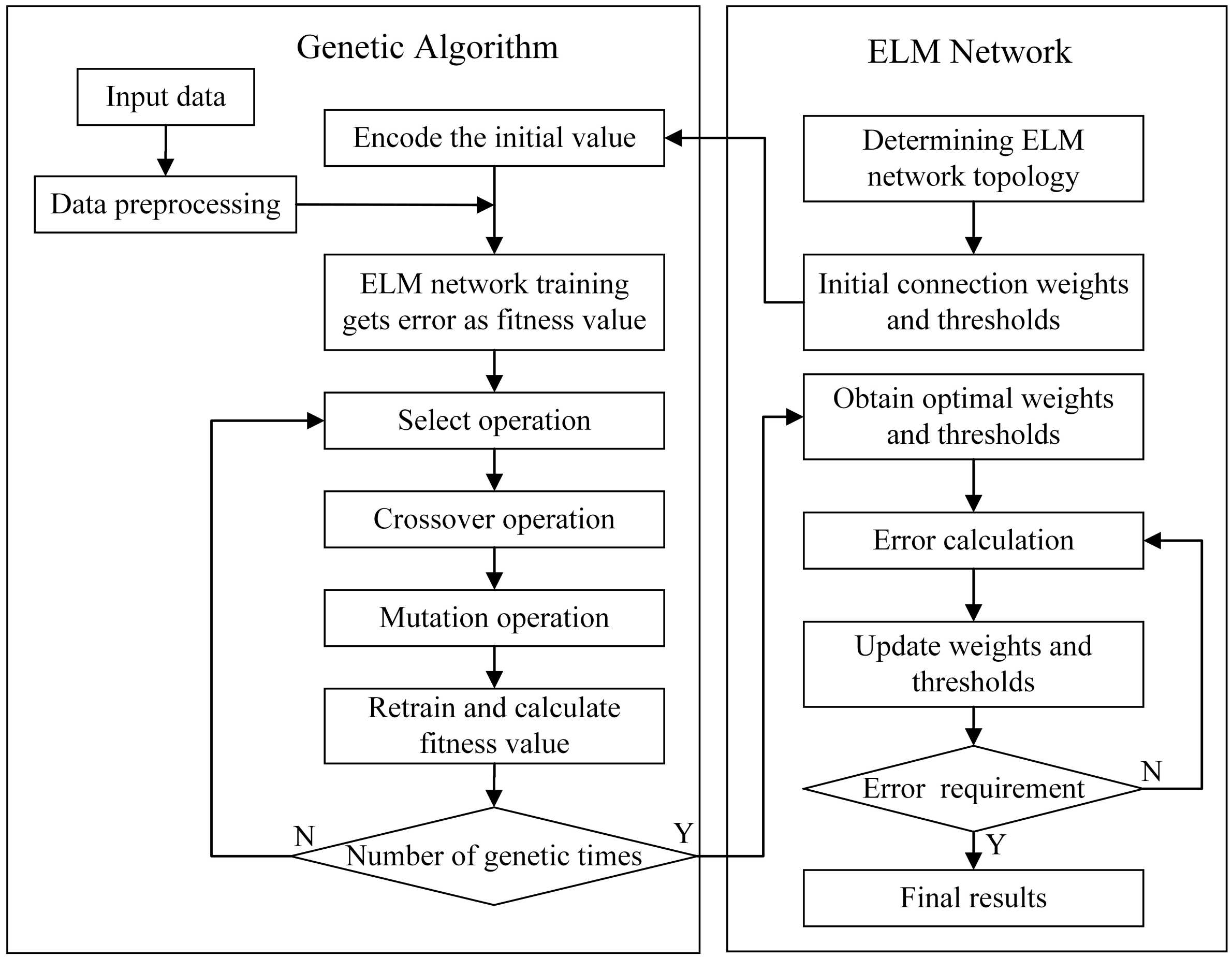
When optimizing the ELMSS and ELMPS models, the genetic algorithm first encodes the connection weights and thresholds of the model to form a certain number of individuals, and then sets the solutions that may have optimal solution individuals to form the population to be optimized. After the population is formed, individuals are screened through selection, crossover, and mutation operations according to the selected fitness function to complete a generation of evolution. Each generation retains the individual with the best fitness value, and generation-by-generation evolution produces approximate solutions with smaller and smaller errors. The flowchart of genetic-algorithm-optimized prediction models is shown in Figure 8.
When performing a selection operation, the fitness function of the individual should be calculated first, and the calculation method is
Among them, X is the predicted value of the sample, is the actual value of the sample, and N is the number of samples in the test set.
Then, the probability that an individual is selected to remain in the next generation is
The crossover operation is to select a part of variables in two individuals to exchange at the same chromosome position. The k individual a and the l individual a crossover at position j as follows:
Among them, b is a random number between 0 and 1, and the probability of crossover between each generation is 0.7.
The mutation operation is that an individual itself mutates at a certain chromosome position. The mutation operation of the i individual at position j is as follows
Among them, g is the current evolutionary generation, G is the maximum evolutionary generation, a and a are the maximum and minimum values of variables in the individual, respectively, and r is a random number between 0 and 1, and the probability of mutation between each generation is 0.01.
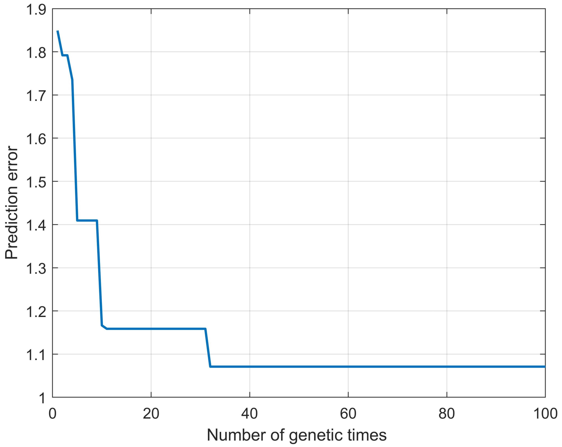
In ELMSS optimized by genetic algorithm (GA-ELMSS), the maximum number of genetic iterations is set to 100, and the change process of prediction errors are shown in Figure 9.
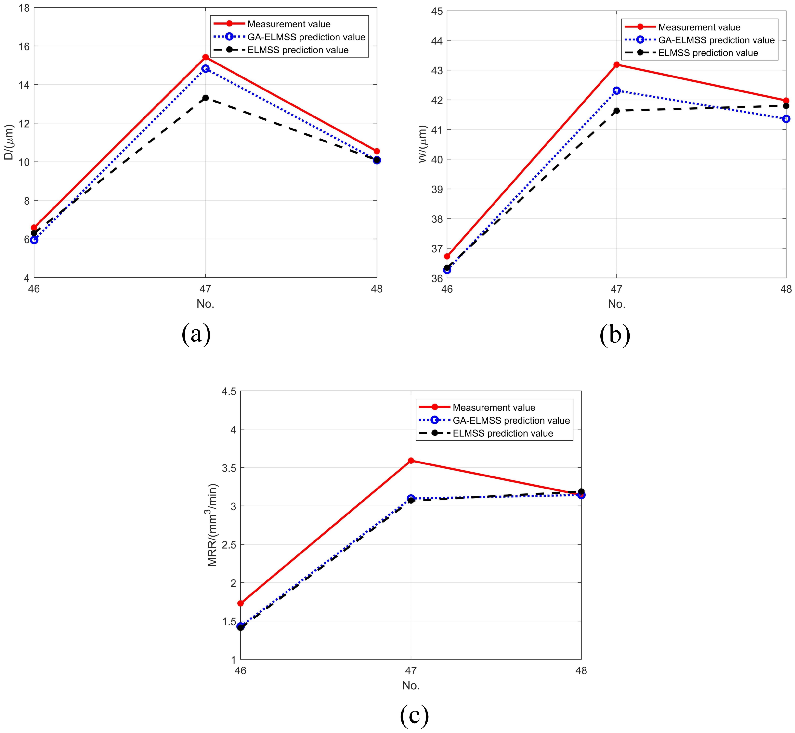
The connection weights and thresholds of GA-ELMSS are shown in Table A2 of Appendix A. At this point, all of the parameters of the ELMSS have been determined, which can be directly applied to the prediction of single-pass machining. Groups 1–45 of data in Table A1 of Appendix A are treated as the training set, and groups 46–48 as the test set. The comparison of the prediction results of the ELMSS before and after the optimization of the genetic algorithm on D, W and MRR are shown in Figure 10.
The prediction accuracies are calculated according to Equation (12), and the results are shown in Table 8. It was found that the genetic algorithm can further improve the prediction accuracies of the GA-ELMSS.
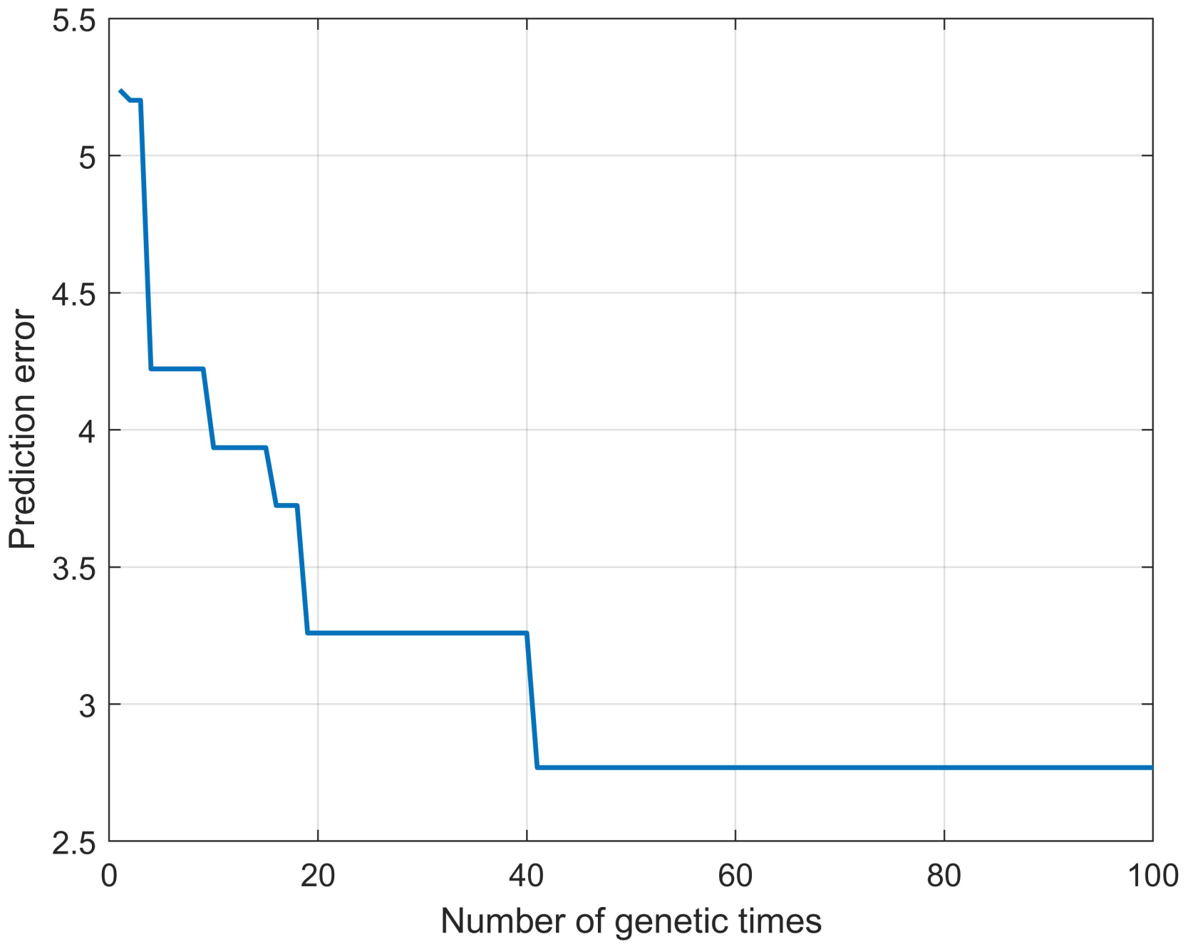
In ELMPS optimized by genetic algorithm (GA-ELMPS), the maximum number of genetic iterations is also set to 100, and the change process of prediction errors are shown in Figure 11.
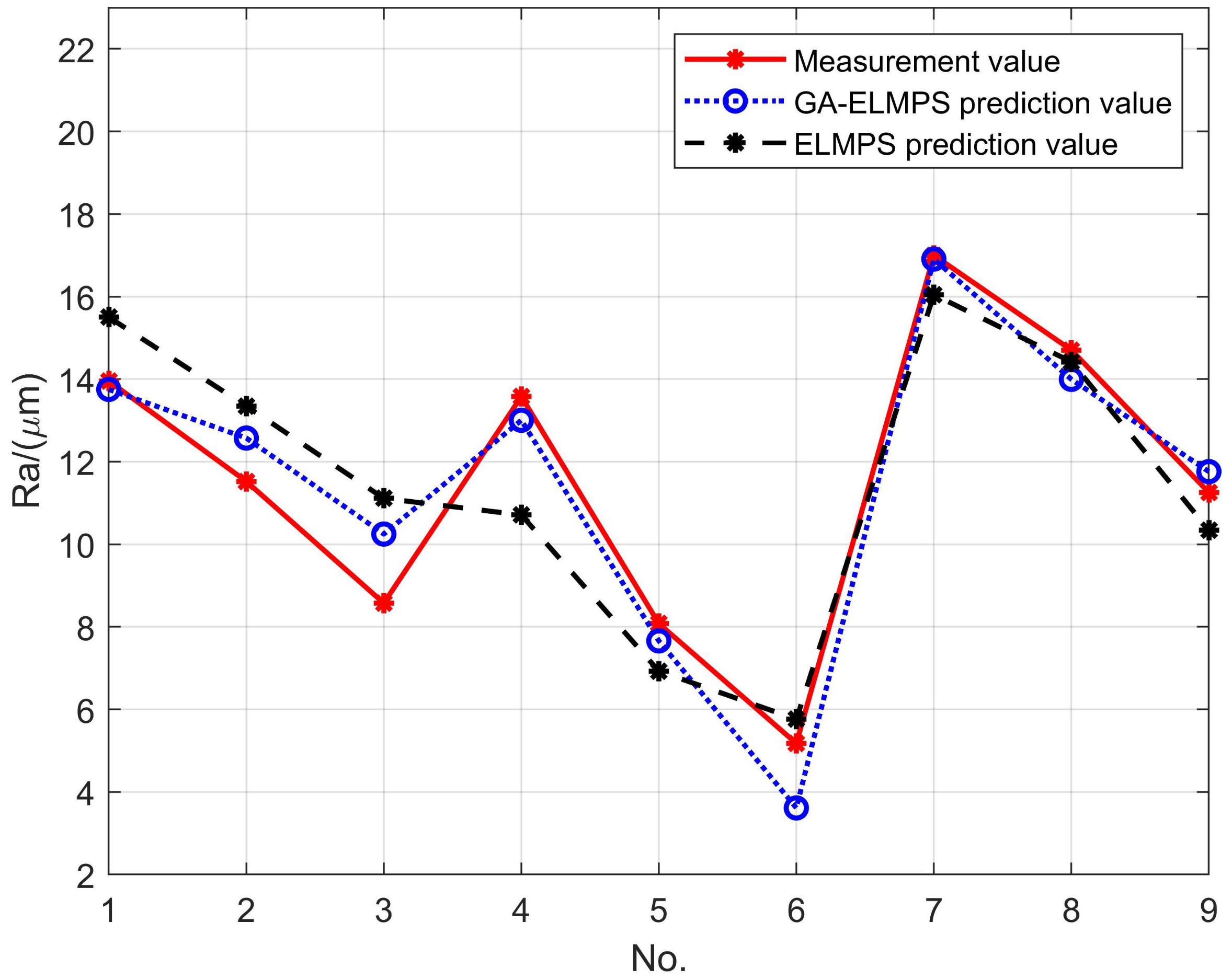
The connection weights and thresholds of GA-ELMSPS are shown in Table A3 of Appendix A. Similarly, groups 1–45 of data in Table A1 of Appendix A are treated as the training set, and groups 46–48 as the test set. The comparison of the prediction results of the ELMPS before and after the optimization of the genetic algorithm on Ra are shown in Figure 12.
6. Conclusions
Surface feature prediction models for laser ablated 40Cr13 stainless steel based on ELM are proposed in this paper. The results of D, W, and MRR processed by single-track scanning were predicted by the ELMSS model, and the results of Ra processed by plane scanning were predicted by the ELMPS model. The prediction accuracy and algorithm efficiency of the proposed models are superior to the BP [16] and RBF [12] neural networks. The main conclusions are summarized as follows:
- The ELMSS model has the highest prediction accuracy for the W, with an average prediction accuracy of 98.3%, followed by D and MRR, which are 92.6% and 92.4%, respectively. Meanwhile, the prediction accuracy for Ra of ELMPS is relatively low, with an average prediction accuracy of 86.8%. Therefore, the models proposed in this paper are relatively more suitable for predicting surface feature of single-pass scanning.
- The prediction accuracies of the ELMSS and ELMPS are higher than that of the BP and RBF neural networks. The prediction accuracies for D were 92.6%, 89.8%, and 89.6% for the ELMSS, BP, and RBF neural networks, respectively; they were 98.3%, 97.4%, and 96.1% for W, respectively; they were 92.4%, 91.1%, and 89.1% for MRR, respectively. The prediction accuracies for Ra were 86.8%, 80.7%, and 79.5% for the ELMPS, BP, and RBF neural networks, respectively. In general, the prediction accuracies of the models proposed in this paper are higher than those of the above two traditional ANN models.
- The computation time of the ELMSS and ELMPS model is significantly lower than that of the other two machine learning methods. In terms of computational efficiency, the models can be ordered as ELMPS, ELMSS, RBF, and BP neural network. Moreover, the computation time of the model proposed in this paper is at the millisecond level, which can be used for the real-time control of laser processing scenarios.
- Through genetic algorithm optimization, the prediction accuracies of ELMSS and ELMPS are further improved. The prediction accuracies of D, W, and MRR are improved from 92.6%, 98.3%, and 92.4% to 94.0%, 99.0%, and 93.2%, respectively. The prediction accuracy of Ra is improved from 86.8% to 91.2%.
In this study, ELMSS and ELMPS were used for the first time in the field of laser processing to accurately predict the features of the ablated surface. With the support of these two models, the results of surface features can be predicted in advance before processing, allowing appropriate process parameters to be selected. Operators do not need much experience or time for experimentation to produce a desirable product. Further, the algorithms of ELMSS and ELMPS are extremely efficient, and determining how to apply them to real-time control will be studied in the future.
Author Contributions
Conceptualization, Z.Y.; Methodology, Z.Y.; Software, P.S. and Z.N.; Validation, Z.Y. and Z.N.; Investigation, Y.Z.; Data curation, Z.Y. and P.S.; Writing—original draft, Z.Y.; Writing—review & editing, Y.Z.; Supervision, Q.L.; Funding acquisition, Q.L. All authors have read and agreed to the published version of the manuscript.
Funding
This research was funded by the National Key Research and Development Program of China (Grant No. 2016YFB1102503).
Institutional Review Board Statement
Not applicable.
Informed Consent Statement
Not applicable.
Data Availability Statement
The research data was provided in Appendix A.
Acknowledgments
The first author would like to express his thanks to Xiuxu W. for offering valuable support during the writing of this manuscript.
Conflicts of Interest
The authors declare no conflict of interest.
Abbreviations
The following abbreviations are used in this manuscript:
| ELMSS | Extreme learning machine of single-track scanning |
| ELMPS | Extreme learning machine of plane scanning |
| MRR | Material removal rate |
| BP | Back propagation |
| RBF | Radial basis function |
| ANN | Artificial neural network |
| LP | Laser power |
| PF | Pulse frequency |
| SS | Scan speed |
| LS | Line spacing |
| D | Depth of ablation |
| W | Width of ablation |
| Ra | Surface roughness |
| GA-ELMSS | ELMSS optimized by genetic algorithm |
| GA-ELMPS | ELMPS optimized by genetic algorithm |
Appendix A

Table A1.
Results of the technological test.
| No. | LP/(W) | PF/(kHz) | SS/(mm/s) | D/(μm) | W/(μm) | MRR/(mm3/min) | LS/(μm) | Ra/(μm) |
|---|---|---|---|---|---|---|---|---|
| 1 | 10 | 40 | 100 | 4.710 | 36.320 | 1.105 | - | - |
| 2 | 10 | 40 | 150 | 3.504 | 35.470 | 1.166 | - | - |
| 3 | 10 | 40 | 200 | 2.710 | 32.544 | 1.391 | - | - |
| 4 | 10 | 40 | 250 | 2.040 | 31.157 | 1.457 | - | - |
| 5 | 10 | 50 | 100 | 5.928 | 37.769 | 1.149 | 5 | 27.794 |
| 10 | 23.326 | |||||||
| 15 | 18.695 | |||||||
| 6 | 10 | 50 | 150 | 4.841 | 36.310 | 1.268 | 5 | 14.293 |
| 10 | 11.015 | |||||||
| 15 | 10.664 | |||||||
| 7 | 10 | 50 | 200 | 3.700 | 33.166 | 1.529 | 5 | 11.764 |
| 10 | 9.155 | |||||||
| 15 | 6.584 | |||||||
| 8 | 10 | 50 | 250 | 3.170 | 32.032 | 1.885 | - | - |
| 9 | 10 | 60 | 100 | 8.365 | 38.769 | 1.291 | 5 | 19.704 |
| 10 | 16.624 | |||||||
| 15 | 12.283 | |||||||
| 10 | 10 | 60 | 200 | 5.044 | 33.660 | 1.829 | 5 | 12.804 |
| 10 | 10.180 | |||||||
| 15 | 8.278 | |||||||
| 11 | 10 | 60 | 250 | 4.044 | 32.320 | 1.997 | - | - |
| 12 | 10 | 70 | 100 | 9.453 | 40.204 | 1.776 | 5 | 14.742 |
| 10 | 12.070 | |||||||
| 15 | 10.263 | |||||||
| 13 | 10 | 70 | 150 | 7.580 | 39.810 | 2.191 | 5 | 14.869 |
| 10 | 13.097 | |||||||
| 15 | 12.301 | |||||||
| 14 | 10 | 70 | 200 | 5.624 | 38.395 | 2.582 | 5 | 11.748 |
| 10 | 7.905 | |||||||
| 15 | 4.838 | |||||||
| 15 | 10 | 70 | 250 | 4.243 | 33.837 | 2.608 | - | - |
| 16 | 14 | 40 | 100 | 7.476 | 40.408 | 1.975 | - | - |
| 17 | 14 | 40 | 150 | 6.130 | 38.708 | 1.916 | - | - |
| 18 | 14 | 40 | 200 | 4.288 | 35.245 | 1.914 | - | - |
| 19 | 14 | 40 | 250 | 3.052 | 32.096 | 1.573 | - | - |
| 20 | 14 | 50 | 100 | 8.146 | 41.272 | 2.184 | 5 | 32.925 |
| 10 | 28.327 | |||||||
| 15 | 23.591 | |||||||
| 21 | 14 | 50 | 150 | 6.348 | 39.048 | 2.039 | 5 | 19.979 |
| 10 | 15.159 | |||||||
| 15 | 12.959 | |||||||
| 22 | 14 | 50 | 200 | 5.549 | 36.511 | 2.066 | 5 | 13.526 |
| 10 | 11.306 | |||||||
| 15 | 8.105 | |||||||
| 23 | 14 | 50 | 250 | 4.746 | 33.123 | 1.794 | - | - |
| 24 | 14 | 60 | 100 | 10.268 | 42.599 | 2.629 | 5 | 21.251 |
| 10 | 18.972 | |||||||
| 15 | 14.757 | |||||||
| 25 | 14 | 60 | 150 | 9.102 | 40.871 | 2.474 | 5 | 17.993 |
| 10 | 15.614 | |||||||
| 15 | 12.274 | |||||||
| 26 | 14 | 60 | 200 | 8.812 | 37.007 | 2.500 | 5 | 13.877 |
| 10 | 11.260 | |||||||
| 15 | 8.337 | |||||||
| 27 | 14 | 60 | 250 | 7.024 | 34.157 | 2.341 | - | - |
| 28 | 14 | 70 | 100 | 17.312 | 43.919 | 3.184 | 5 | 17.849 |
| 10 | 13.181 | |||||||
| 15 | 11.067 | |||||||
| 29 | 14 | 70 | 200 | 10.878 | 39.783 | 3.062 | 5 | 15.051 |
| 10 | 14.290 | |||||||
| 15 | 12.107 | |||||||
| 30 | 14 | 70 | 250 | 7.965 | 35.157 | 2.669 | - | - |
| 31 | 18 | 40 | 100 | 14.575 | 46.128 | 2.603 | - | - |
| 32 | 18 | 40 | 150 | 9.374 | 43.166 | 2.333 | - | - |
| 33 | 18 | 40 | 200 | 7.041 | 41.972 | 2.258 | - | - |
| 34 | 18 | 40 | 250 | 5.231 | 37.051 | 2.333 | - | - |
| 35 | 18 | 50 | 100 | 20.385 | 49.208 | 3.802 | 5 | 35.821 |
| 10 | 30.670 | |||||||
| 15 | 25.005 | |||||||
| 36 | 18 | 50 | 150 | 12.270 | 45.340 | 3.043 | 5 | 22.010 |
| 10 | 19.117 | |||||||
| 15 | 14.139 | |||||||
| 37 | 18 | 50 | 200 | 8.811 | 40.191 | 2.674 | 5 | 14.345 |
| 10 | 10.596 | |||||||
| 15 | 9.437 | |||||||
| 38 | 18 | 50 | 250 | 6.703 | 38.369 | 2.668 | - | - |
| 39 | 18 | 60 | 100 | 25.609 | 51.713 | 4.905 | 5 | 29.545 |
| 10 | 22.808 | |||||||
| 15 | 19.132 | |||||||
| 40 | 18 | 60 | 150 | 14.685 | 47.270 | 3.649 | 5 | 19.415 |
| 10 | 17.802 | |||||||
| 15 | 13.063 | |||||||
| 41 | 18 | 60 | 250 | 8.321 | 39.969 | 3.108 | - | - |
| 42 | 18 | 70 | 100 | 33.557 | 58.532 | 5.783 | 5 | 20.487 |
| 10 | 18.945 | |||||||
| 15 | 15.735 | |||||||
| 43 | 18 | 70 | 150 | 17.000 | 52.575 | 4.280 | 5 | 19.233 |
| 10 | 15.224 | |||||||
| 15 | 13.599 | |||||||
| 44 | 18 | 70 | 200 | 12.086 | 42.954 | 3.708 | 5 | 14.304 |
| 10 | 10.192 | |||||||
| 15 | 6.231 | |||||||
| 45 | 18 | 70 | 250 | 9.282 | 40.840 | 3.301 | - | - |
| 46 | 10 | 60 | 150 | 6.590 | 36.341 | 1.730 | 5 | 13.956 |
| 10 | 11.522 | |||||||
| 15 | 8.573 | |||||||
| 47 | 14 | 70 | 150 | 15.415 | 41.633 | 3.591 | 5 | 13.578 |
| 10 | 8.079 | |||||||
| 15 | 5.176 | |||||||
| 48 | 18 | 60 | 200 | 10.545 | 41.798 | 3.144 | 5 | 16.999 |
| 10 | 14.704 | |||||||
| 15 | 11.253 |
Table A2.
The connection weights and thresholds of GA-ELMSS.
| IW1 | IW2 | IW3 | B | LW1 | LW2 | LW3 |
|---|---|---|---|---|---|---|
| −0.232 | −0.086 | 0.031 | 0.079 | −1826.213 | −4082.110 | −1450.281 |
| −0.036 | 0.481 | −0.430 | −0.080 | −220.138 | 639.136 | 201.555 |
| 0.089 | −0.113 | −0.101 | 0.125 | −754.249 | −291.58 | −908.682 |
| 0.432 | −0.440 | −0.442 | −0.318 | −245.316 | 299.979 | 106.916 |
| 0.172 | −0.472 | −0.481 | 0.408 | 472.233 | −633.298 | −283.131 |
| 0.274 | −0.045 | 0.040 | −0.303 | 630.142 | −2520.600 | −1486.372 |
| −0.009 | −0.293 | 0.339 | 0.087 | −1177.209 | 2947.502 | 830.049 |
| −0.182 | 0.265 | 0.287 | 0.158 | −99.858 | 1920.822 | 1213.711 |
| 0.453 | 0.198 | 0.193 | −0.302 | 3093.931 | 154.709 | 651.381 |
| 0.374 | −0.185 | −0.143 | −0.395 | −987.277 | 1859.971 | 1085.935 |
| 0.240 | −0.489 | 0.032 | −0.206 | −51.833 | 438.757 | −96.488 |
| 0.452 | 0.131 | 0.052 | −0.227 | −4406.521 | −4427.502 | −1876.558 |
| 0.463 | 0.105 | 0.115 | −0.352 | 3389.136 | 2832.371 | 1202.500 |
| −0.484 | 0.432 | 0.292 | −0.205 | −52.638 | −57.240 | 158.769 |
| −0.169 | −0.348 | −0.213 | 0.351 | −15.892 | −520.897 | −243.700 |
| −0.203 | −0.067 | −0.440 | 0.002 | 1529.101 | −1179.513 | −207.149 |
| 0.087 | −0.031 | 0.457 | 0.396 | 1066.204 | −1399.417 | −492.390 |
| 0.235 | −0.435 | −0.292 | −0.160 | −3468.958 | 5082.055 | 1747.812 |
| 0.232 | 0.321 | 0.499 | −0.435 | 386.744 | −298.529 | −139.302 |
| −0.202 | 0.250 | −0.022 | −0.219 | 730.832 | −362.843 | −550.227 |
| 0.424 | −0.442 | −0.199 | 0.105 | 487.610 | −1254.683 | −173.397 |
| 0.419 | 0.433 | −0.449 | −0.047 | 8.212 | 43.563 | 23.585 |
| −0.298 | 0.012 | 0.418 | −0.119 | −820.394 | 242.580 | 129.553 |
| −0.087 | 0.384 | 0.308 | 0.138 | −807.174 | 369.732 | −260.524 |
| 0.292 | −0.443 | −0.308 | −0.431 | 2302.590 | −3053.327 | −1091.668 |
| 0.014 | −0.059 | −0.435 | 0.336 | −2022.303 | 974.542 | −17.184 |
| −0.344 | 0.227 | −0.344 | 0.490 | −330.872 | 306.562 | 90.751 |
| −0.306 | 0.424 | −0.235 | −0.060 | 265.001 | 58.001 | −103.546 |
| 0.412 | −0.015 | 0.473 | 0.339 | −67.134 | 35.861 | 74.545 |
| 0.112 | 0.357 | −0.145 | −0.063 | −770.724 | 1100.53 | 153.023 |
| −0.339 | −0.163 | −0.256 | 0.458 | 4189.418 | 395.267 | 695.384 |
| 0.302 | −0.149 | −0.289 | 0.401 | 228.638 | 313.967 | 661.793 |
| −0.281 | 0.311 | −0.056 | −0.484 | −791.866 | −99.713 | 237.574 |
Table A3.
The connection weights and thresholds of GA-ELMPS.
| IW1 | IW2 | IW3 | IW4 | B | LW |
|---|---|---|---|---|---|
| 0.004 | 0.329 | −0.126 | −0.178 | −0.163 | −284.652 |
| −0.107 | −0.283 | 0.479 | −0.377 | 0.166 | 72.062 |
| 0.054 | 0.217 | 0.460 | 0.478 | −0.063 | 223.608 |
| 0.268 | −0.160 | 0.072 | −0.436 | −0.078 | 108.983 |
| −0.077 | −0.183 | −0.328 | −0.016 | 0.384 | −765.715 |
| 0.282 | −0.212 | 0.372 | 0.265 | 0.473 | 101.259 |
| 0.141 | 0.114 | −0.388 | 0.483 | −0.047 | −29.873 |
| −0.332 | −0.045 | 0.000 | −0.101 | −0.357 | −206.184 |
| −0.130 | −0.093 | 0.449 | −0.024 | −0.444 | 205.914 |
| −0.478 | −0.421 | 0.016 | 0.458 | −0.359 | 86.762 |
| −0.136 | 0.419 | −0.296 | 0.338 | 0.300 | −39.310 |
| −0.438 | −0.444 | 0.060 | −0.464 | 0.315 | 4.860 |
| 0.065 | 0.229 | 0.036 | −0.385 | −0.140 | 829.225 |
| −0.221 | −0.239 | −0.309 | 0.249 | 0.352 | 104.030 |
| −0.498 | −0.139 | −0.026 | 0.086 | -0.185 | 14.744 |
| 0.296 | 0.142 | −0.451 | −0.393 | 0.294 | −100.834 |
| 0.040 | −0.401 | −0.364 | 0.462 | 0.283 | 65.728 |
| 0.009 | −0.332 | 0.089 | −0.316 | −0.161 | −29.440 |
| 0.447 | −0.344 | −0.036 | 0.423 | −0.430 | −13.284 |
| −0.300 | −0.242 | 0.151 | -0.168 | 0.258 | 286.638 |
| 0.159 | −0.120 | −0.320 | −0.184 | -0.491 | −179.574 |
| −0.126 | 0.346 | −0.370 | −0.334 | -0.330 | 124.116 |
| 0.482 | −0.279 | −0.428 | −0.458 | 0.363 | −42.063 |
| −0.114 | −0.170 | −0.264 | −0.353 | 0.090 | 353.406 |
| −0.115 | −0.424 | 0.141 | 0.400 | 0.472 | 173.414 |
| 0.375 | 0.412 | −0.382 | 0.357 | −0.377 | 15.628 |
| −0.059 | 0.418 | 0.472 | 0.413 | 0.349 | −13.191 |
| −0.455 | 0.037 | 0.043 | −0.326 | 0.170 | −91.091 |
| 0.489 | 0.406 | 0.122 | −0.114 | 0.374 | −2.451 |
| −0.198 | −0.154 | 0.344 | 0.417 | 0.443 | −96.488 |
| 0.408 | 0.394 | 0.495 | 0.015 | −0.361 | −22.932 |
| 0.223 | 0.000 | −0.036 | −0.443 | −0.132 | −87.396 |
| 0.335 | −0.011 | −0.457 | −0.438 | 0.167 | 17.290 |
| −0.156 | −0.367 | 0.013 | 0.121 | 0.053 | −274.688 |
| −0.385 | 0.389 | −0.056 | 0.336 | 0.038 | 92.504 |
| 0.003 | 0.050 | 0.352 | 0.114 | -0.316 | −976.839 |
| −0.118 | −0.468 | −0.442 | −0.493 | −0.184 | 16.016 |
| −0.006 | −0.369 | 0.065 | −0.355 | −0.455 | −29.808 |
| −0.360 | 0.100 | −0.079 | 0.470 | 0.385 | 59.787 |
| 0.469 | −0.158 | −0.029 | 0.290 | 0.430 | 8.016 |
| −0.397 | −0.284 | −0.463 | 0.335 | −0.451 | −5.219 |
| 0.299 | −0.187 | −0.302 | −0.258 | 0.390 | 430.767 |
| 0.230 | −0.247 | −0.348 | −0.330 | −0.481 | 52.736 |
| −0.449 | −0.335 | −0.095 | −0.291 | −0.252 | −28.102 |
| 0.242 | 0.335 | −0.153 | 0.148 | -0.499 | 382.970 |
| 0.200 | 0.195 | −0.296 | 0.399 | 0.223 | 315.188 |
| 0.263 | −0.169 | −0.306 | −0.164 | 0.433 | −388.675 |
| −0.087 | −0.205 | 0.009 | 0.383 | −0.149 | 768.795 |
| −0.130 | −0.061 | 0.041 | −0.144 | −0.242 | −344.754 |
| −0.122 | −0.457 | −0.013 | 0.079 | 0.500 | 209.373 |
| 0.058 | −0.459 | 0.412 | 0.381 | −0.076 | −28.213 |
| −0.429 | −0.280 | 0.448 | 0.253 | −0.443 | −95.304 |
| 0.307 | 0.317 | −0.284 | 0.274 | −0.013 | −160.962 |
| −0.199 | 0.492 | −0.056 | 0.221 | 0.103 | −186.473 |
| −0.492 | −0.151 | 0.492 | −0.442 | 0.206 | −7.225 |
| −0.264 | −0.303 | −0.027 | 0.469 | −0.215 | −216.882 |
| 0.240 | −0.370 | 0.181 | −0.164 | 0.197 | −129.670 |
| 0.290 | 0.373 | 0.242 | 0.382 | 0.140 | −24.274 |
| 0.458 | 0.018 | −0.049 | 0.213 | 0.191 | −308.920 |
| 0.139 | −0.232 | 0.395 | 0.333 | −0.406 | 59.406 |
References
- Bonse, J.; Kirner, S.; Griepentrog, M.; Spaltmann, D.; Krüger, J. Femtosecond Laser Texturing of Surfaces for Tribological Applications. Materials 2018, 11, 801. [Google Scholar] [CrossRef] [PubMed] [Green Version]
- Nsilani Kouediatouka, A.; Ma, Q.; Liu, Q.; Mawignon, F.J.; Rafique, F.; Dong, G. Design Methodology and Application of Surface Texture: A Review. Coatings 2022, 12, 1015. [Google Scholar] [CrossRef]
- Wu, B.; Deng, L.; Liu, P.; Zhang, F.; Duan, J.; Zeng, X. Effects of picosecond laser repetition rate on ablation of Cr12MoV cold work mold steel. Appl. Surf. Sci. 2017, 409, 403–412. [Google Scholar] [CrossRef]
- Rung, S.; Häcker, N.; Hellmann, R. Micromachining of Alumina Using a High-Power Ultrashort-Pulsed Laser. Materials 2022, 15, 5328. [Google Scholar] [CrossRef] [PubMed]
- Sun, H.; Li, J.; Liu, M.; Yang, D.; Li, F. A Review of Effects of Femtosecond Laser Parameters on Metal Surface Properties. Coatings 2022, 12, 1596. [Google Scholar] [CrossRef]
- Wang, X.; Duan, J.; Jiang, M.; Zhang, F.; Ke, S.; Wu, B.; Zeng, X. Investigation of processing parameters for three-dimensional laser ablation based on Taguchi method. Int. J. Adv. Manuf. Technol. 2017, 93, 2963–2974. [Google Scholar] [CrossRef]
- Mills, B.; Grant-Jacob, J.A. Lasers that learn: The interface of laser machining and machine learning. IET Optoelectron. 2021, 15, 207–224. [Google Scholar] [CrossRef]
- Chen, Y.; Wang, H.; Wu, Y.; Wang, H. Predicting the Printability in Selective Laser Melting with a Supervised Machine Learning Method. Materials 2020, 13, 5063. [Google Scholar] [CrossRef]
- Yousef, B.F.; Knopf, G.K.; Bordatchev, E.V.; Nikumb, S.K. Neural network modeling and analysis of the material removal process during laser machining. Int. J. Adv. Manuf. Technol. 2003, 22, 41–53. [Google Scholar] [CrossRef]
- Teixidor, D.; Grzenda, M.; Bustillo, A.; Ciurana, J. Modeling pulsed laser micromachining of micro geometries using machine-learning techniques. J. Intell. Manuf. 2015, 26, 801–814. [Google Scholar] [CrossRef]
- Jimin, C.; Jianhua, Y.; Shuai, Z.; Tiechuan, Z.; Dixin, G. Parameter optimization of non-vertical laser cutting. Int. J. Adv. Manuf. Technol. 2007, 33, 469–473. [Google Scholar] [CrossRef]
- Niu, B.; Chen, J.; Liu, F. Optimization on the Fiber Laser Micro-Cutting of Thin Stainless Steel Sheet by Artificial Neural Networks. Adv. Sci. Lett. 2011, 4, 810–813. [Google Scholar] [CrossRef]
- Dhupal, D.; Doloi, B.; Bhattacharyya, B. Optimization of process parameters of Nd:YAG laser microgrooving of Al2TiO5 ceramic material by response surface methodology and artificial neural network algorithm. Proc. Inst. Mech. Eng. Part J. Eng. Manuf. 2007, 221, 1341–1350. [Google Scholar] [CrossRef]
- Dixit, S.R.; Das, S.R.; Dhupal, D. Parametric optimization of Nd:YAG laser microgrooving on aluminum oxide using integrated RSM-ANN-GA approach. J. Ind. Eng. Int. 2019, 15, 333–349. [Google Scholar] [CrossRef] [Green Version]
- Ciurana, J.; Arias, G.; Ozel, T. Neural Network Modeling and Particle Swarm Optimization (PSO) of Process Parameters in Pulsed Laser Micromachining of Hardened AISI H13 Steel. Mater. Manuf. Process. 2009, 24, 358–368. [Google Scholar] [CrossRef]
- Dhara, S.K.; Kuar, A.S.; Mitra, S. An artificial neural network approach on parametric optimization of laser micro-machining of die-steel. Int. J. Adv. Manuf. Technol. 2008, 39, 39–46. [Google Scholar] [CrossRef]
- Yin, Z.; Liu, Q.; Sun, P.; Wang, J. Study on Nanosecond Laser Ablation of 40Cr13 Die Steel Based on ANOVA and BP Neural Network. Appl. Sci. 2021, 11, 10331. [Google Scholar] [CrossRef]
- Dubey, A.K.; Yadava, V. Laser beam machining—A review. Int. J. Mach. Tools Manuf. 2008, 48, 609–628. [Google Scholar] [CrossRef]
- Huang, G.-B.; Zhu, Q.-Y.; Siew, C.-K. Extreme learning machine: A new learning scheme of feedforward neural networks. In Proceedings of the 2004 IEEE International Joint Conference on Neural Networks (IEEE Cat. No.04CH37541), Budapest, Hungary, 25 July 2004; Volume 2, pp. 985–990. [Google Scholar] [CrossRef]
- Huang, G.B.; Zhu, Q.Y.; Siew, C.K. Extreme learning machine: Theory and applications. Neurocomputing 2006, 70, 489–501. [Google Scholar] [CrossRef]
- Huang, G.; Song, S.; Gupta, J.N.D.; Wu, C. Semi-Supervised and Unsupervised Extreme Learning Machines. IEEE Trans. Cybern. 2014, 44, 2405–2417. [Google Scholar] [CrossRef]
- Zhu, Q.Y.; Qin, A.; Suganthan, P.; Huang, G.B. Evolutionary extreme learning machine. Pattern Recognit. 2005, 38, 1759–1763. [Google Scholar] [CrossRef]
Figure 1.
The experimental platform.

Figure 2.
The laser pulse accumulation diagram of single-pass machining.

Figure 3.
The laser pulse accumulation diagram of plane scanning.

Figure 4.
Schematic of machining results and measurement process. (a) Typical micro-groove diagram observed by LEXT OLS5100. (b) Section profile of the micro-groove. (c) Physical image of the rough surface after plane scanning. (d) Typical surface morphology observed by LEXT OLS5100.
Figure 4.
Schematic of machining results and measurement process. (a) Typical micro-groove diagram observed by LEXT OLS5100. (b) Section profile of the micro-groove. (c) Physical image of the rough surface after plane scanning. (d) Typical surface morphology observed by LEXT OLS5100.

Figure 5.
Typical single hidden layer neural network structure.

Figure 6.
Prediction models for surface features based on ELM. (a) ELMSS model for feature prediction. (b) ELMPS model for feature prediction.
Figure 6.
Prediction models for surface features based on ELM. (a) ELMSS model for feature prediction. (b) ELMPS model for feature prediction.

Figure 7.
Absolute error between the predicted value and actual value of the three types of models. (a) Absolute error of D of three types of models. (b) Absolute error of W of three types of models. (c) Absolute error of MRR of three types of models. (d) Absolute error of Ra of three types of models.

Figure 8.
The flowchart of genetic algorithm optimized prediction models.

Figure 9.
The change process of prediction errors of GA-ELMSS.

Figure 10.
Comparison of the prediction results of the GA-ELMSS. (a) The prediction results of GA-ELMSS for D. (b) The prediction results of the GA-ELMSS for W. (c) The prediction results of GA-ELMSS for MRR.
Figure 10.
Comparison of the prediction results of the GA-ELMSS. (a) The prediction results of GA-ELMSS for D. (b) The prediction results of the GA-ELMSS for W. (c) The prediction results of GA-ELMSS for MRR.

Figure 11.
The change process of prediction errors of GA-ELMPS.

Figure 12.
The prediction results of the GA-ELMPS on Ra.

Table 1.
Main components of 40Cr13 stainless steel (wt%).
| C | Si | Mn | S | P | Cr | Ni |
|---|---|---|---|---|---|---|
| 0.36–0.45 | ≤0.60 | ≤0.80 | ≤0.03 | ≤0.035 | 12.00–14.00 | ≤0.60 |
Table 2.
Main parameters of laser generator.
| Wavelength | Maximum Power | M2 Factor | Spot Diameter | Pulse Width | Repetition Rate |
|---|---|---|---|---|---|
| 355 nm | 25 W | 1.2 | 19.38 μm | <20 ns | 40–300 kHz |
Table 3.
Process parameters of single-track scanning.
| Process Parameters | Range of Values | |||
|---|---|---|---|---|
| LP/(W) | 10 | 14 | 18 | |
| PF/(kHz) | 40 | 50 | 60 | 70 |
| SS/(mm/s) | 100 | 150 | 200 | 250 |
Table 4.
Process parameters of plane scanning.
| Process Parameters | Range of Values | ||
|---|---|---|---|
| LP/(W) | 10 | 14 | 18 |
| PF/(kHz) | 50 | 60 | 70 |
| SS/(mm/s) | 100 | 150 | 200 |
| LS/(μm) | 5 | 10 | 15 |
Table 5.
Measured value and prediction results of the three types of models.
| No. | D/(μm) | W/(μm) | MRR/(mm3/min) | |||||||||
|---|---|---|---|---|---|---|---|---|---|---|---|---|
| BP | RBF | ELMSS | Exp. | BP | RBF | ELMSS | Exp. | BP | RBF | ELMSS | Exp. | |
| 46 | 6.222 | 7.140 | 6.302 | 6.590 | 37.754 | 36.617 | 36.727 | 36.341 | 1.627 | 1.465 | 1.611 | 1.730 |
| 47 | 11.718 | 12.924 | 13.313 | 15.415 | 41.407 | 43.985 | 43.184 | 41.633 | 2.996 | 3.137 | 3.070 | 3.591 |
| 48 | 10.447 | 11.256 | 10.087 | 10.545 | 43.236 | 39.542 | 41.974 | 41.798 | 3.280 | 3.290 | 3.188 | 3.144 |
Table 6.
Measured values and prediction results of Ra.
| No. | Ra/(μm) | |||
|---|---|---|---|---|
| BP | RBF | ELMPS | Exp. | |
| 46-1 | 14.735 | 15.804 | 15.500 | 13.956 |
| 46-2 | 12.886 | 12.819 | 13.347 | 11.522 |
| 46-3 | 10.754 | 11.779 | 11.112 | 8.573 |
| 47-1 | 12.497 | 11.552 | 10.709 | 13.578 |
| 47-2 | 9.771 | 9.427 | 6.927 | 8.079 |
| 47-3 | 6.860 | 5.646 | 5.762 | 5.176 |
| 48-1 | 13.802 | 12.968 | 16.045 | 16.999 |
| 48-2 | 11.149 | 10.843 | 14.419 | 14.704 |
| 48-3 | 8.322 | 7.675 | 10.342 | 11.253 |
Table 7.
Training time of the three types of models.
| BP | RBF | ELMSS | ELMPS | |
|---|---|---|---|---|
| Single-track scanning | 1.896 s | 0.147 s | 0.005 s | - |
| Plane scanning | 1.208 s | 0.211 s | - | 0.002 s |
Table 8.
Prediction accuracies of ELMSS and GA-ELMSS.
| ELMSS | GA-ELMSS | |
|---|---|---|
| D | 92.6% | 94.0% |
| W | 98.3% | 99.0% |
| MRR | 92.4% | 93.2% |
Table 9.
Prediction accuracies of ELMPS and GA-ELMPS.
| ELMPS | GA-ELMPS | |
|---|---|---|
| Ra | 86.8% | 91.2% |
Disclaimer/Publisher’s Note: The statements, opinions and data contained in all publications are solely those of the individual author(s) and contributor(s) and not of MDPI and/or the editor(s). MDPI and/or the editor(s) disclaim responsibility for any injury to people or property resulting from any ideas, methods, instructions or products referred to in the content. |
© 2023 by the authors. Licensee MDPI, Basel, Switzerland. This article is an open access article distributed under the terms and conditions of the Creative Commons Attribution (CC BY) license (https://creativecommons.org/licenses/by/4.0/).
Share and Cite
MDPI and ACS Style
Yin, Z.; Liu, Q.; Sun, P.; Zhou, Y.; Ning, Z. Surface Feature Prediction for Laser Ablated 40Cr13 Stainless Steel Based on Extreme Learning Machine. Materials 2023, 16, 505. https://doi.org/10.3390/ma16020505
AMA Style
Yin Z, Liu Q, Sun P, Zhou Y, Ning Z. Surface Feature Prediction for Laser Ablated 40Cr13 Stainless Steel Based on Extreme Learning Machine. Materials. 2023; 16(2):505. https://doi.org/10.3390/ma16020505
Chicago/Turabian StyleYin, Zhenshuo, Qiang Liu, Pengpeng Sun, Yinuo Zhou, and Zhiwei Ning. 2023. "Surface Feature Prediction for Laser Ablated 40Cr13 Stainless Steel Based on Extreme Learning Machine" Materials 16, no. 2: 505. https://doi.org/10.3390/ma16020505
Note that from the first issue of 2016, this journal uses article numbers instead of page numbers. See further details here.