
Unsupervised Machine Learning Techniques for Improving Reservoir Interpretation Using Walkaway VSP and Sonic Log Data


1
Department of Geoinformatics and Applied Computer Science, Faculty of Geology, Geophysics and Environmental Protection, AGH University of Science and Technology, 30-059 Krakow, Poland
2
Department of Fossil Fuels, Faculty of Geology, Geophysics and Environmental Protection, AGH University of Science and Technology, 30-059 Krakow, Poland
*
Author to whom correspondence should be addressed.
Energies 2023, 16(1), 493; https://doi.org/10.3390/en16010493
Submission received: 27 November 2022
/
Revised: 23 December 2022
/
Accepted: 26 December 2022
/
Published: 2 January 2023
(This article belongs to the Special Issue Geophysics, Geomechanics, Drilling Mechanics and Seepage Mechanics of Unconventional Oil and Gas Reservoirs)
Abstract
:In this paper, we present a detailed analysis of the possibility of using unsupervised machine learning techniques for reservoir interpretation based on the parameters obtained from geophysical measurements that are related to the elastic properties of rocks. Four different clustering algorithms were compared, including balanced iterative reducing and clustering using hierarchies, the Gaussian mixture model, k-means, and spectral clustering. Measurements with different vertical resolutions were used. The first set of input parameters was obtained from the walkaway VSP survey. The second one was acquired in the well using a full-wave sonic tool. Apart from the study of algorithms used for clustering, two data pre-processing paths were analyzed in the context of matching the vertical resolution of both methods. The validation of the final results was carried out using a lithological identification of the medium based on an analysis of the drill core. The measurements were performed in Silurian rocks (claystone, mudstone, marly claystone) lying under an overburdened Zechstein formation (salt and anhydrite). This formation is known for high attenuating seismic signal properties. The presented study shows results from the first and only multilevel walkaway VSP acquisition in Poland.
1. Introduction
Currently, oil exploration requires a comprehensive analysis and the highest standards both at the stage of data processing and at the stage of geophysical and reservoir interpretation. The search for smaller and smaller oil and gas deposits, as well as increasing environmental pressure, forces the optimization of acquisition techniques, which, in turn, translates into an increased effort toward the next stages (data processing and geophysical interpretation) of the subsurface identification process. The use of new data processing techniques, including anisotropy analysis or dedicated processing techniques for data re-processing, is becoming a new standard [1,2,3]. It has been proved that anisotropy analysis is crucial even for static calculation [4,5], and also that structure-oriented processing can give new, valuable information about deep layers [6]. The need for new techniques at the stage of interpretation is also noticeable. Intensive research has been carried out in order to find new solutions or develop existing solutions. One option is to use machine learning (ML) and artificial intelligence (AI). Information from different profiling can show new, valuable divisions of the rock complexes, which are hard to distinguish using the classical approach. The oil and gas industry is entering a new era of digital transformation. The use of ML and AI is a core foundation of this new path. Combining them with a dedicated processing approach can be a game-changer for modern and future exploration, allowing for reducing exploration costs and environmental hazards.
ML is a powerful automatic computing tool based on numerical and logical operations that is able to learn from examples or find hidden patterns in datasets [7,8]. Regarding the most common and also basic principles, ML can be divided into supervised and unsupervised learning. In the supervised one, the data are labeled and the prediction is made based on input and output datasets. In other words, the output is known as a priori to create a model, and then the model is used with the new input data for making predictions. Unsupervised ML does not need labeled data and output datasets to make a model as this type of learning is based only on the input dataset. Unsupervised learning is used for labeling data. One example of unsupervised learning is clustering. There are many clustering algorithms available in popular ML libraries of Python or R.
In this paper, we studied the use of unsupervised ML for clustering based on walkaway VSP and sonic log data for improving reservoir interpretation. Data were collected in Northern Poland as a part of a bigger project focused on shale gas exploration [9,10]. The walkaway VSP data were very noisy. The four different processing schemas were investigated to obtain the best possible results. In this paper, we used P-wave inclination angles from a 4 km offset range obtained from data processed according to the flow published in [3]. The inclination angles are characterized by very small errors (in a window with a width approximately equal to the wavelength). We also used anisotropy parameters—Alkhalifah and Tsvankin’s anellipticity coefficient [11] and Thomsen’s anisotropic coefficient [12]—obtained from walkaway VSP measurements using the P-wave only inversion method introduced by [13]. A detailed study of the calculation of these parameters can be found in [9]. Besides walkaway VSP measurement-based parameters, we also used sonic log delay times and the Poisson ratio with lithology identifier (calculated from sonic). Our motivation was to check if the clustering based on measurements associated with the elastic properties of rocks can be used in reservoir interpretation in the case of shale gas exploration. We examined four different algorithms available in the scikit-learn library [14]. As the evaluation of the clustering process is not a trivial task, we used the core lithology interpretation for the results evaluation. However, this is not the only difficulty and unknown in these studies. Besides clustering evaluation and cluster numbers setting, there is also a problem associated with different scales of walkaway VSP and well-log measurements. We checked both cases—downscaling (from a lower to higher resolution) VSP measurements (step 15 m) to a sonic-log resolution (0.1 m) and upscaling (from higher to lower resolution) the sonic-log measurements to the walkaway VSP step. In the case of downscaling, the distances between successive points are reduced, whereas, in the case of upscaling, these distances are increased. Without detailed research, it is difficult to say which will bring better results. On the one hand, a larger number of observations should have a positive effect on the clustering process, but on the other hand, borehole profiling is characterized by significant noise and requires smoothing in order not to introduce an excessive amount of outliers.
The paper contains a brief description of the local geology (Section 2). In Section 3, a detailed explanation of clustering algorithms, together with metrics that can help to decide the number of clusters, is described. Section 4 consists of an explanation of processing techniques and geophysical measurements used for feature dataset preparation. Additionally, a discussion about the problem of combining the resolutions for sonic and borehole seismic activity is presented. In Section 5, the well W-1 case study results are shown. An interpretation of the clustering results is presented in Section 6 and then, in the final part (Section 7), the paper is summarized and concluded.
2. Region Characterization
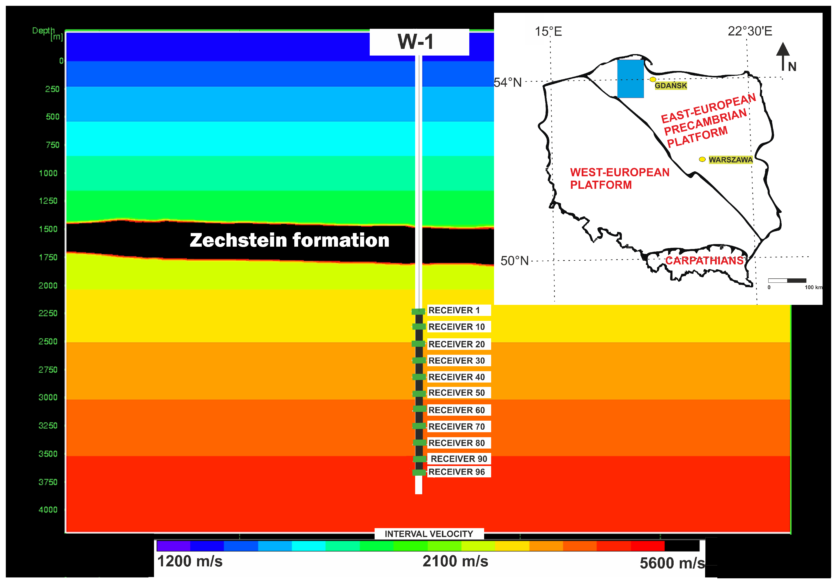
Presented data were acquired in 2016 in Poland as a part of a shale gas exploration project called “Polish Technologies for Shale Gas”. Walkaway VSP data acquisition was performed during very harsh weather conditions in November. The W-1 project was located in the Northern Poland Kashubian Lake District [15]. It is also a part of the Eastern-European Precambrian Platform. A more detailed description is the central-western part of the Baltic Syneclise, located at the eastern side of the Łeba elevation [16]. The terrain morphology is mainly related to glacial processes. The young glacial nature of the moraine plateau with frequent frontal hills (with an absolute height of nearly 160 m measured depth from ground level (MDGL) as well as a relative height of approximately 30 m) and many glacial gutters (often with lakes) is common in the studied area. The main river in this region is the Wierzyca river, where numerous peat-boggy depressions are present [3]. On the crystalline rocks, Permo-Mesozoic and Lower Paleozoic structural complexes occur. Deposition starts with alluvial sediments (with alluvial fans) of the Żarnowiec formation (Lower Paleozoic). Along with Lower and Middle Cambrian sediments, they are counted as one big meso-sedimentary complex. The presence of Upper Cambrian rocks is very rare as, in general, they are incredibly eroded. Ordovician and Silurian rock complexes are placed directly on the Cambrian layers. Both hold many breaks initiated by changing conditions between erosion and sedimentation periods. Zechstein’s formation of evaporites rocks is a part of the Upper Permian complex. These rocks are known for their properties, which are a significant obstacle in the geophysical recognition of rocks lying beneath them [9]. The Mesozoic series starts with Lower Triassic sediments of sandstone, claystone, and mudstone. Carbonate intercalations often occur in this series. Directly over these rocks, the Muschelkalk is present (Middle Triassic). It consists of dolomite, marl, and limestone. Cretaceous deposits are located successively. Lower Cretaceous consists of marly limestones and glauconite sandstones, whereas Upper Cretaceous consists of marls. Miocene formations represent tertiary rock sediments (mostly marly clays and sand silt). Quaternary rocks are exemplified by gravel sediments and glacial sand with frequent pebbles [17]. In the W-1 survey region, the three main sealing complexes were distinguished. Ludlow and Pridoli complexes are made of claystone and silt with an extremely low permeability and porosity. The Zechstein sealing complex is very thick—in some places, the thickness is over 400 m. This formation is built of anhydrite and salt with a very high P-wave velocity (average 6000 m/s). The location of the W-1 well and the velocity model used for the seismic depth migration is shown in Figure 1.
3. Unsupervised Machine Learning Methods
Clustering is an example of an unsupervised ML scheme relying on grouping datasets on clusters based on the similarity between particular points. Clustering is one of the core features of ML [18], but also of AI [19], data mining [20], and even in compression [21]. There are many different clustering methods created for different purposes, including memory optimization, consisting shapes, similarity measurement metrics, etc. [22]. In this paper, four popular clustering methods were studied: balanced iterative reducing and clustering using hierarchies (BIRCH), the Gaussian mixture model (GM), k-means, and the spectral clustering (SPCL) method.
3.1. BIRCH Clustering
BIRCH is an unsupervised clustering method that is known not only for its suitability for dealing with big datasets but also for its little sensitivity to noise in the data [23]. This method can be easily scalable as the compressed representation of the input dataset is utilized by using the clustering feature tree (CFT). Each clustering feature (CF) can be linked with summarized statistics that can be easily and dynamically implemented with the new data. Scalability is indisputability a feature that clearly separates this algorithm from the other algorithms analyzed in this paper. In the multi-level process, the BIRCH algorithm first accumulates input data into a tree structure whose size is significantly reduced compared to the original data. The lean data representation from the first step is used for clustering in the second step. The main contribution of BIRCH is a flexible logic for aggregating the data so that an informative representation is retained even when the size is substantially reduced [24].
- Step 1 First scan. In this step, the whole dataset examination is performed to create the initial CFT.
- Step 2 Reorganization of the initial CFT if it is too long.
- Step 3 Adapted agglomerative global hierarchical clustering is performed to create sub-clusters.
- Step 4 This is an optional step that allows for other scans to improve and redefine the current structure.
Besides scalability and noise reduction advantages, the BIRCH also has disadvantages. One of the main disadvantages is that BIRCH works fine with clusters with shapes close to hyper-spherical as the radius is used for the clusters’ border regulations. The BIRCH algorithm was an inspiration for many others, such as data bubbles, CluStream, two-step clustering, and DenStream. In 2006, the BIRCH approach won the Time Award in the SIGMOD test [24]. Undoubtedly, this approach, due to its easy scalability even with very limited resources, may be a good option when multiple logs with a high vertical resolution and sampling are considered for clustering.
3.2. Gaussian Mixture Model Clustering
Gaussian distribution, which is also called normal distribution, is the probability distribution broadly used for scientific purposes when random continuous variable modeling is considered. Starting from a very simple one-dimensional example, the Gaussian distribution is defined according to Equation (1):
where is a variable with a real value, is the simple mean of all observations, and is variance. For the case where the mean is equal to 0 and variance is equal to 1, the symmetry axis of the distribution is the vertical y-axis. For a more complex case, in D-dimensional space, the Gaussian distribution for vector is defined as in Equation (2):
where represents the covariance matrix (dimension D × D), is the mean vector (D-dimensional), and denotes the determinant of the covariance matrix. Although the Gaussian distribution is one of the most often used for analytical purposes, due to its symmetry, it is not suitable for multimodal data characterized by complex density regions as it is extremely challenging to capture the frame of superposition of two or more Gaussians with a single Gaussian distribution. To overcome this limitation, mixture distribution is used. This probabilistic model was described by [25] and the study was expanded in the following years [26,27]. The technique used for unsupervised machine learning clustering is based on the probability model and is called the Gaussian mixture (GM) model. This method is based on the expectation-maximization technique for the determination of ellipsoidal clusters based on probability density estimates. Each superposition of the k-Gaussian probability distributions, which is, in fact, the linear combination of these distributions, can be described as according to Equation (3):
where is a mean of each Gaussian component in a mixture, is its covariance, represents the mixing coefficient, and they sum up to 1 for normalized Gaussian components of . When , for all k and , mixing coefficients can be described by probabilities and the margin density can be calculated using Equation (4):
Considering N observations that are identically distributed and independent, the likelihood function is given by Equation (5):
Indeed, the presented situation for mixed Gaussians is appreciably more complicated than the situation for a single Gaussian distribution. However, the use of the natural logarithm function in Equation (5) prevents statistical underflow for many numbers of relatively small probabilities. A calculation of this likelihood has no form of analytical solution, but, rather, it is an iterative optimization solution [28,29]. To overcome this computation problem (for finding maximum likelihood models for latent variables) the expectation-maximization algorithm can be used [30]. The typical EM algorithm after [31] is:
- Step 1 Initialization for and evaluation of the initial likelihood.
- Step 2 This is the expectation step where the responsibilities are evaluated using the parameters’ values from the previous step.
- Step 3 This is the maximization step where the processes of parameter re-estimation are performed with the use of responsibilities from the expectation step.
- Step 4 Likelihood evaluation—if the convergence measure is satisfied, the algorithm ends; if not, another loop starting from step 2 is performed until the criterion is satisfied.
3.3. K-Means Clustering
K-means is a non-probabilistic approach based on a simple calculation of squared Euclidean distance values [32]. For a given a priori number of clusters, the inner-cluster distance between points is minimized, whereas the distances between points in different clusters are maximized. Let us consider data points in a D-dimensional space. Our goal is to group them into a given M number of clusters. To measure the distance, the D-dimensional vectors’ set for the range needs to be set. These vectors are related to cluster centers. The k-means goal is to find data points and correspond vector sets to them where the squared distance value is the smallest. The similarity E is the Euclidean distance calculated according to Equation (6):
where and . Similar to the GM model, k-means also uses the EM approach for assigning dataset points into particular clusters. The typical algorithm after [31] is:
- Step 1 Random M centroid initialization.
- Step 2 This is the expectation step where the distance computation between each data point and each centroid is calculated. Points are assigned to the closest cluster.
- Step 3 This is the maximization step where the mean for each cluster is calculated and then the centroids are updated.
- Step 4 The number of iterations is checked to see if it is reached or if there is no difference in cluster assignment. If it is reached, it is the end of the algorithm; if not, step 2 is carried out.
K-means is one of the most popular clustering algorithms due to its easy implementation and very high performance [33]. However, there are also a couple of disadvantages. The first is related to the clusters number that needs to be set a priori. It is often difficult to set up optimal cluster numbers without knowledge of the data’s nature. Secondly, while a particular data point is at a similar distance to more than one cluster, there is no option to handle the problem of uncertainty. Thirdly, clusters could be very unsatisfactory if non-linear decision boundaries are present in the dataset.
3.4. Spectral Clustering
This is a frequently used method of clustering with a solid theoretical foundation. According to the study in [34], three main advantages of SPCL can be stated. The first is related to the mentioned solid foundation based on the algebraic theory of spectral graphs. The second advantage is associated with the possibility of the determination of a very complex cluster’s structure. Finally, the third one is related to computation complexity. The computation time for SPCL is polynomial. Opposite to k-means and GM, SPCL can easily handle datasets with a non-convex structure without collapsing into the local minimum or maximum [35]. In this type of clustering, there is no need to scan the structure of the dataset globally, which can be an advantage in the case of parallelism [36]. As mentioned before, the basics of this clustering algorithm are algebraic spectral graph theory. Clusters are created in a line with a graph partitioning process. First, the undirected graph is created with all dataset points counted as a vertex. The similarity measure between points is the weight of the edge linking the two vertexes. Typical SPCL algorithm after [37]:
- Step 1 Calculation of the similarity matrix S. An undirected, weighted graph is used as the whole dataset representation. Each vertex represents data point K and the weighted value M at the edge connection is used for the similarity measurement. The undirected weighted graph is created according to the similarity measurement between points (it is a graph partitioning problem). The adjacency matrix is used as graph information representation.
- Step 2 Calculation of the diagonal matrix D. The similarity between each point and all other points is represented by
- Step 3 Calculation of the non-normalized Laplace matrix . Each row of the matrix L contains information about both similarities between points and the sum of all similarities. This allows for preserving information in the graph.
- Step 4 Eigenvalues calculation. In this step, the p-smallest eigenvectors of the Laplace matrix are found and then the corresponding eigenvalues are calculated.
- Step 5 Creation of orthogonal matrix O, using vectors obtained in previous step.
- Step 6 Performance of clustering over normalized row vectors obtained in the previous step using k-means.
For SPCL, many different cut-off criteria were introduced to overcome the minimum cut criterion limitation (only for a simple, convex distribution). Also currently in use are the ratio-cut, max-min-cut, ratio-cut, multiway-normalized-cut, normalized-cut, and others [34].
3.5. Validation of the Number of Clusters
The estimation of the optimal number of clusters is neither easy nor unambiguous. There are many different techniques used to specify the optimal value of a cluster based on internal, external, or relative techniques [38].
3.5.1. Silhouette Coefficient
We used the silhouette coefficient (SC) Equation (7), which shows the similarity between particular points within the particular cluster to the points in this cluster and how much they differ from points in other clusters. The silhouette coefficient range is from −1 to 1, where −1 indicates the worst number of clusters, and 1 indicates the best number [39]. SC is calculated according to this formula [14]:
where
- —Silhouette coefficient;
- a—The mean distance between the point and other points inside the cluster;
- b—The distance between a point and the nearest cluster (to which this point does not belong).
3.5.2. Davies–Bouldin Index
The Davies–Bouldin index (DB) is based on the similarity between clusters that are supposed to have a data density that is decreasing with the distance from a vector characteristic of the particular cluster. This method was described by Davies and Bouldin in 1979 [40]. A better result is obtained for clusters that are characterized by a lower dispersion and greater distance between clusters. On the graph, the values that are closer to zero represent the optimum number of clusters. It should be remembered that the index is overstated for convex clusters compared to clusters characterized by a different structure, and the use of the distance measure forces the limitation to the Euclidean space. The DB is calculated using Equation (8):
where,
- —Davies-Bouldin index;
- —Cluster diameter—the average distance between the i-cluster centroid and points in this cluster;
- —Cluster diameter—the average distance between the j-cluster centroid and points in this cluster;
- —The distance between i and j cluster centroids.
3.5.3. Calinski–Harabasz Index
The Calinski–Harabasz index (CH) is called the variance ratio criterion and was introduced by [41]. The basic criterion for calculating this index is the ratio between the total dispersion within a given cluster and between clusters. Dispersion here is specified as a summed squared distance. This index is very fast to calculate and gives higher values for separated and dense clusters. Let us consider k clusters over the W dataset (with size ). The CH can be calculated [14,41] using Equation (9):
where
- —The trace of the covariance matrix (between groups);
- —The trace of the covariance matrix (within the cluster).
3.6. Inertia Analysis
Inertia allows for the measurement of body resistance to moving it around a particular point. In clustering, the inertia of a particular point refers to the sum of squared distances in Euclidean space with respect to their mass center. Increasing the mass of the points and also the distance will result in an increase in inertia. For the X point cloud, the total inertia can be described as using Equation (12) [42]:
where
- —The center of mass defined as ;
- —The i-point;
- —The weight of the i-point.
Computing this measure with a different number of clusters gives a graph where the transition zone from vertical to plateau is visible. The point of transition indicates the optimal number of clusters.
3.6.1. Bayesian Information Criterion
For clustering methods evaluation, the information criterion can be used for the estimation of the optimal number of clusters. The Bayesian information criterion (BIC) is an example of one of them. The BIC penalty is data-independent; however, it is dependent on the number of mixture components. As a consequence, the highest number of possible components can be indicated by this method. On the other hand, it has been proved that BIC gives consistent results [43]. For ML pipelines, the BIC can be calculated using Equation (13) and Laplace approximation of model marginal likelihood , where samples of a finite mixture distribution are stored in [44].
3.6.2. Domain-Based Interpretation
Unsupervised ML techniques are used for finding hidden patterns in data [45]; however, specific domain-based knowledge and good data recognition can help with the evaluation of model parameters [46]. The two main branches of domain-based validation can be described for the exploration of oil and gas needs. The first one is related to the conclusions from the previous, standard investigation (seismic processing, interpretation, and geological structures analysis), and the second is related to the statistical analysis of input parameters. In many papers, domain-based knowledge was the important factor when clustering was considered [47,48]. The authors of [49] proposed the use of mudlogs, core data, other well-logs data, and even region studies about stratigraphy for the validation of ML clusters. Geophysical measurements are the physical response of the rock mass, so it is natural and correct to analyze the results of clustering in the context of the geological structure. The use of various types of measurements of the same wave field, differing in the type of acquisition or the range of source parameters, allows for the observation of macro and micro responses of the rock medium. Clustering can overcome the difficulty in defining the numerical relationship between these parameters. The second mentioned branch is related to a statistical analysis of data. The analysis of distributions and patterns allows for getting acquainted with the general population distribution in advance. Standard techniques of exploratory data analysis (such as kernel density estimation, box plots, swarm plots, and others) can be used [50].
4. Geophysical Methods Characterization
4.1. W-1 Well Dataset
The dataset consists of parameters calculated from the walkaway VSP survey and sonic log measurements. Observations were made in a vertical well located in the north of Poland as a part of Polish technologies for a shale gas project. The aim was to obtain clusters based on measurements based on the elastic wave field measured in different scales to refine and update information on the P-wave velocity model.
4.1.1. Walkaway VSP Measurment
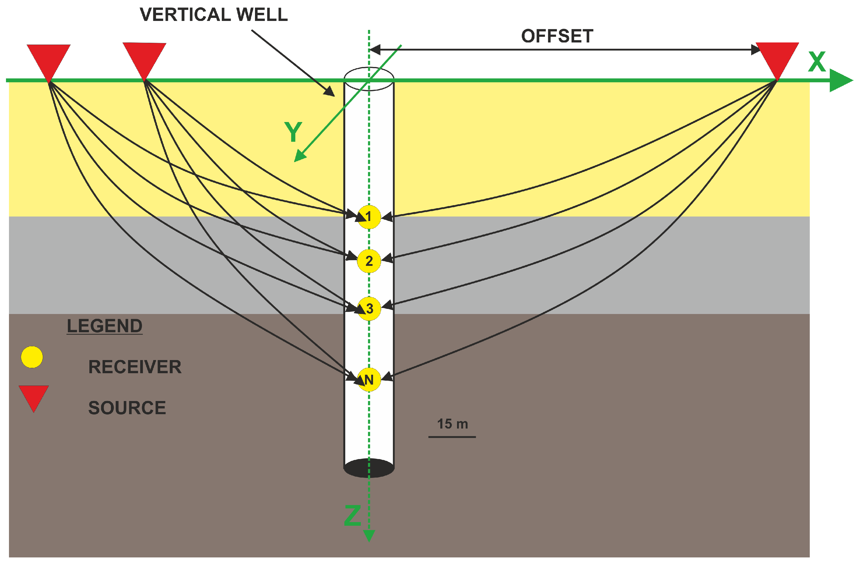
In the case of VSP studies, the sources of elastic waves are located on the Earth’s surface at certain distances from the borehole, along with the profile. The receiver or receivers are located inside the borehole and usually record the field of P-waves and shear waves (Figure 2).
The walkaway VSP measurement in the W-1 well allowed for simultaneous registration in ninety-six BSR 3-C receivers (Oyo Geospace Company). It was the first walk-away measurement in central Europe [9]. Geophones were spaced in a vertical well with a step equal to 15 m. The probe was positioned in the Silurian complex—the first geophone was placed at a depth of 2400 m and the last receiver at a depth of 3825 m MDGL. A total of 480 shot points (SP) were performed along a 12 km profile, with up to 8 sweeps performed on each shot point. The sweep frequency was 6–120 Hz, the length was 16 s, and the recording time was 4 s. Inclination angles obtained from 31 different offsets were used according to Table 1 (where absolute (abs) offsets are listed). The average inclination (avg incl) for a particular shot point is a simple average calculated over all 96 receivers. Using the P-wave-only inversion method, the in situ anisotropy parameters were calculated: Alkhalifah and Tsvankin’s anellipticity coefficient [11] and Thomsen’s anisotropic coefficient [12]. Parameters were inverted only from the P-wave waveform for 94 depth points.
4.1.2. Borhole Sonic Measurment
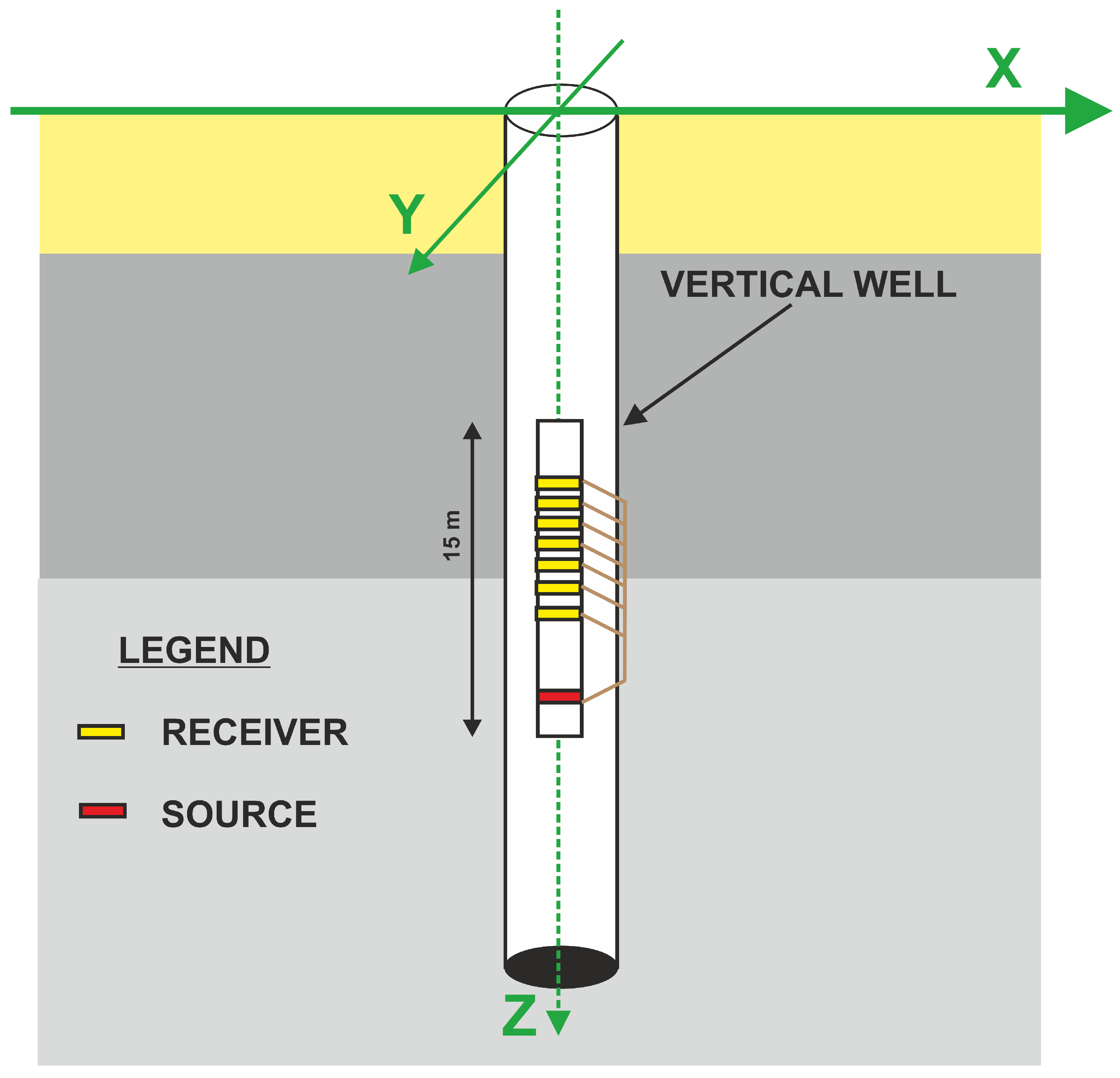
The dipole sonic tool is able to measure velocities of P-, fast, and slow shear waves directly in the well. Sources and receivers are distributed on one device (Figure 3). Due to higher wave frequencies than those emitted in VSP, it is possible to obtain a relatively higher measurement of the vertical resolution. On the other hand, the range is limited to a small zone around the borehole [51].
Measurement points were carried out with a step equal to 0.1 m. The Full Wave sonic tool was used, so it was possible to calculate (P-wave velocity), (sonic wave velocity from the horizontal X-component), and (sonic wave velocity from the horizontal Y-component) using measured delay times: the delay time of the compressional P-wave (), the delay time of the slow shear wave (), and the delay time of the fast shear wave (). We also calculated the shear anisotropy from the sonic acoustic log according to Equation (14), , which is a parameter used as a lithology identifier (Equation (15)), and also the Poisson ratio according to Equation (16). The ratio of to was additionally calculated as one of the input parameters.
where
- —The delay time of the slow shear wave;
- —The delay time of the fast shear wave;
- —The average delay time of the shear wave.
- —The lithology identifier;
- —The sonic wave velocity from the horizontal X-component;
- —The sonic P-wave velocity.
- —The Poisson ratio from the sonic tool;
- —The lithology identifier.
The sonic tool measurements consisted of an observation of 12,751 depth points.
4.1.3. Resolution for Clustering
Choosing the appropriate sampling step for clustering when using parameters of different resolutions is a difficult task. The receivers for walkaway VSP measurements were placed in the well every 15 m, while the measuring step for the sonic tool was 0.1 m. In this case, there are two possible ways of proceeding: upscaling well-logs to the walkaway VSP resolution (experiment 1) or downscaling the walkaway VSP measurements to the well-logs resolution (experiment 2).
- Experiment 1—All parameters were adjusted to the resolution of the walkaway VSP measurements in W-1. This allowed for a significant data reduction and, consequently, for an acceleration of the computational time. On the other hand, fewer points can sometimes have a negative impact on clustering results. The upscaling of well-logs is not a trivial task, and is an interpretation procedure. This will filter out minor variations and leave only the main lithological changes. For this purpose, smoothing filters, Backus averaging, or blocking in the intervals can be used. In this case, the sonic log parameters’ values on the walkaway VSP receiver depth point were calculated as a simple average calculated in the window with a length equal to the P-wavelength centralized on this depth point. A total of 92 observations were obtained for 45 different parameters, which gave a dataset consisting of 4140 data points.
- Experiment 2—All parameters were adjusted to the resolution of the sonic log measurements in W-1. In this case, the number of observations was significantly improved, but, on the other hand, the computation time was also significantly increased. The cubic interpolation method was used for upscaling the walkaway VSP measurements. This procedure is much easier to perform than downscaling the well-log measurements. In experiment 2, sonic log measurements were smoothed using a Savitzky–Golay polynomial filter with a window length equal to 650 samples and a polynomial order of 3. We chose this filter because of its ability to cope with noise, which is undoubtedly present in the profiling of borehole geophysics. This is also a well-established method cited more than 3800× [52]. In this case, a total of 12,751 observations were obtained for 45 different parameters, which gave a dataset consisting of 599,291 data points.
It can be easily noticed that Experiment 2 has almost 140× more data points than experiment 1. This undoubtedly affects the computation time and therefore the cost of the whole process. However, does it have an impact on the final results of the clustering? Can the obtained differences be acceptable within the required accuracy? It should be added that the observations were made in almost homogeneous Silurian sediments. A lithological profile based on the analysis of the drill core was used as a reference point. A final interpretation of the obtained results was carried out in the context of the complex knowledge of the investigated region, which includes conclusions from the 3D seismic study, microseismical observation, and general classic reservoir interpretation. In both experiments, data were standardized as the significant differences between very small values of anisotropic parameters and high values of velocities were present. This procedure allowed us to avoid the artificial domination of measurements with high values compared to other ones. The preprocessing of data was performed using the Python scikit-learn package [14].
5. W-1 Case Study
5.1. Features Description
Correct data preparation is an important step. Removing outliers, reconciling units, scales, and standardization are essential for proper grouping 45. Different elastic parameters were used as the input for clustering tests using BIRCH, GM, k-means, and SPCL algorithms. These parameters were standardized (using Standard Scaler from sklearn.preprocessing library [14]) as their ranges were significantly different. The full list of parameters with their initial values and units in which they were determined is presented in Table 2. It is worth mentioning that the results of machine learning techniques are dependent on the quality of the input data. In this case, despite the extremely difficult acquisition of the VSP and the poor quality of the initial data, thanks to the processing techniques [3], it was possible to obtain high-quality features. For the given depth range, there were no missing values. Due to the measurement specification, as well as the domain shift, outliers were mostly eliminated using a smoothing filter.
5.2. Number of Clusters
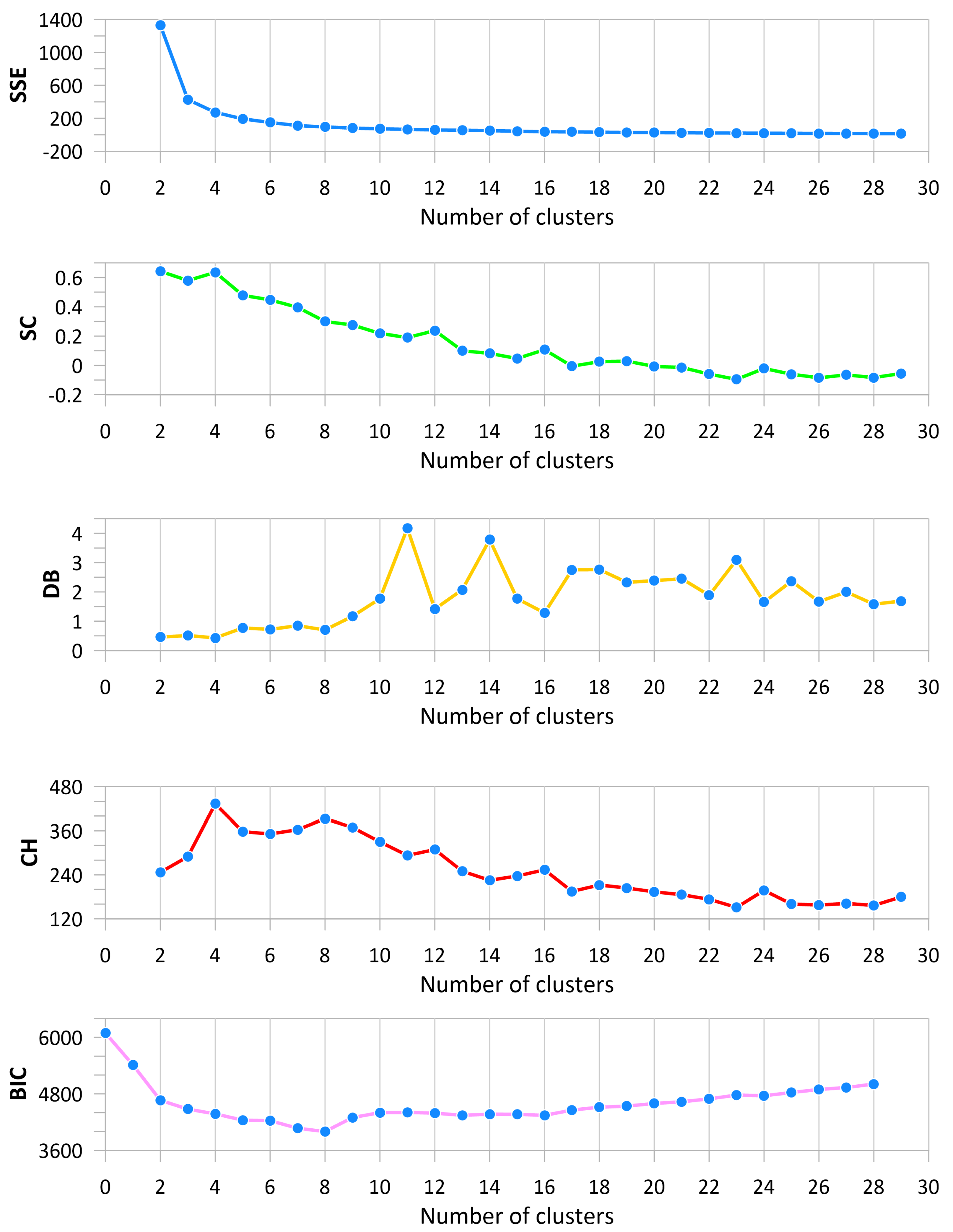
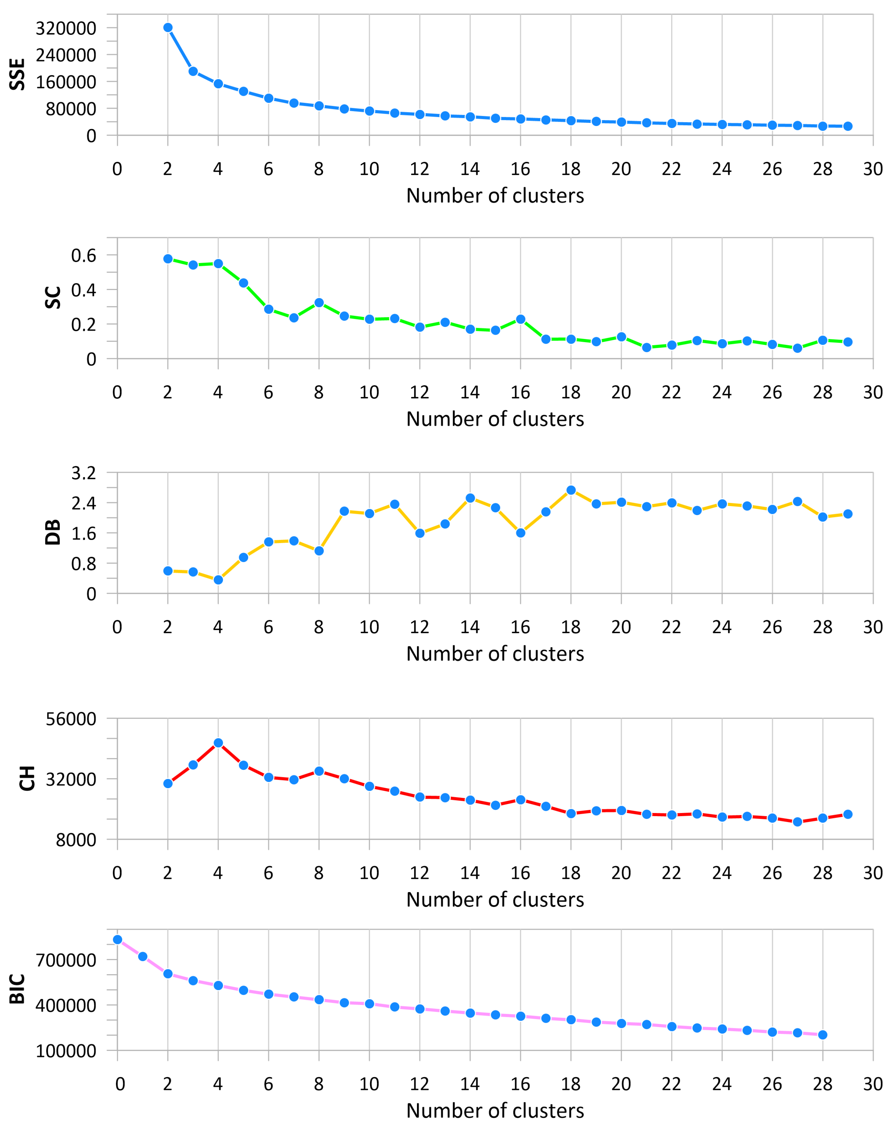
To select the optimal number of clusters, the following metrics were calculated: inertia (SSE—as the sum of squared errors), silhouette coefficient (SC), Davies–Bouldin index (DB), Calinski–Harabasz Index (CH), and Bayesian information criterion (BIC). They were calculated for the k-means algorithm for both scenarios: walkaway VSP resolution (Figure 4) and sonic resolution (Figure 5). As we were looking for the best clusters to correct the initial velocity model, the maximum considered number of clusters was 30. In general values over 20, they would be difficult to interpret, as well as too small for the dominant seismic wavelength. We were looking for a rapid change in the SSE plot, maximum or local maximums in the SC and CH, the local or global minimum for the DB, and the minimum on the BIC curve. For the walkaway VSP resolution (Figure 4), it is clearly visible that BIC indicates that the number of clusters is equal to 8, as this is the global minimum for the function in the analyzed range. The CH global maximum is for n = 4; however, the local maximum can also be observed for . The DB shows local minimums on the graph for . The SC also indicates that the number of clusters is equal to 4, 8, 12, or 16. The SSE is hard to interpret, but we can assume that 4 or 8 will be a good choice based on this metric. For sonic resolution (Figure 5), the BIC does not give a clear answer as to the number of clusters. The DB shows clearly that the optimal number can be 4, 8, 12, or 16. Based on the CH and SC, the best choice would be 4, 8, and 16. The shape of the SSE for sonic resolution is very similar to the one obtained for the walkaway VSP resolution. By analyzing all of these metrics as a whole, assuming no number greater than 20, the following numbers of clusters—4, 8, 12, and 16—were selected for this specific geological target for a further analysis and interpretation of the model results.
6. Clustering Results
6.1. Four Clusters
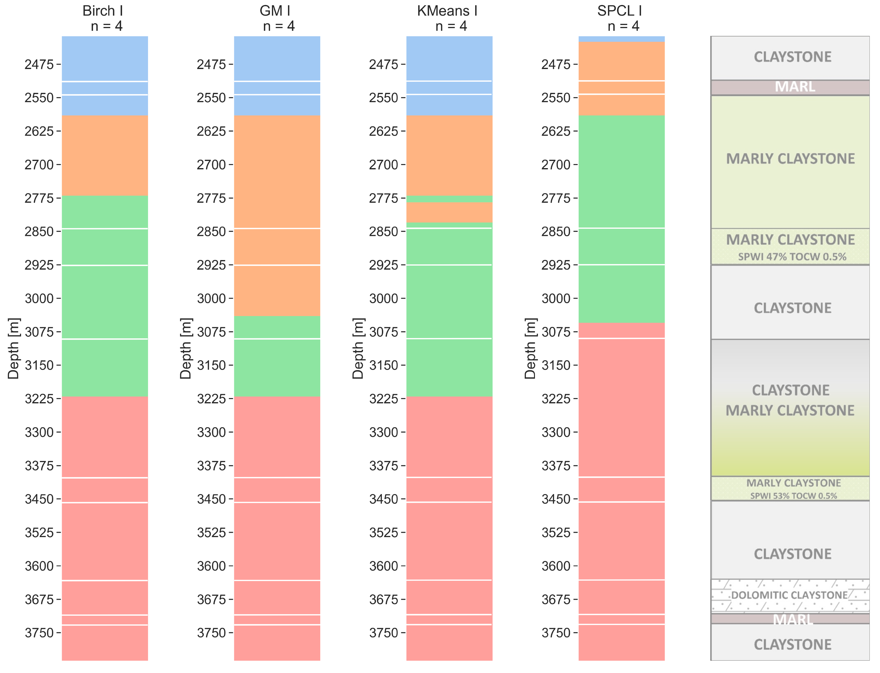
The results obtained for the four clusters are very similar to the initial velocity model used for depth migration. For this model, the four-velocity complexes were divided along the probe length.
For the walkaway VSP resolution (Figure 6), the bottom of the first (blue) and third (green) layer is at the same depth for BIRCH, GM, and k-means, whereas, for SPCL, the first layer is very thin and the bottom of the third layer is at a lower depth compared to the other methods; however, it is at the same depth as the bottom of the claystone layer determined by core analysis. The most similar models are obtained from BIRCH and k-means, with small differences at a depth of 2775 m. Interestingly, the k-means model shows a stratification in this place (above potentially saturated marl). For all models, the last layer is the thicker one.
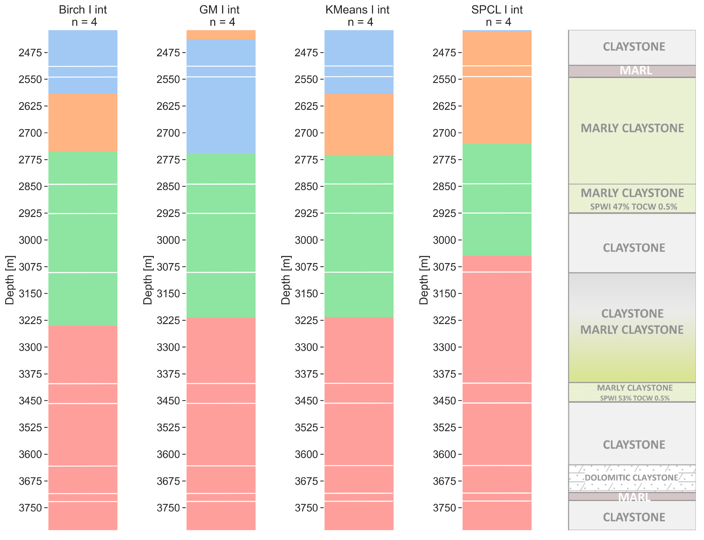
For the sonic resolution (Figure 7), BIRCH and k-means models are again very similar. SPCL effectively gives only three clusters that are in line with the model obtained for the walkaway VSP resolution. The top of layer 3 for all methods is almost at the same depth of 2775 m MDGL. The bottom of this layer for BIRCH, GM, and KM is also at a similar depth: 3225 m MGDL. For SPCL, the bottom of that layer is at the same depth as for the walkaway VSP resolution (3070 m MDGL).
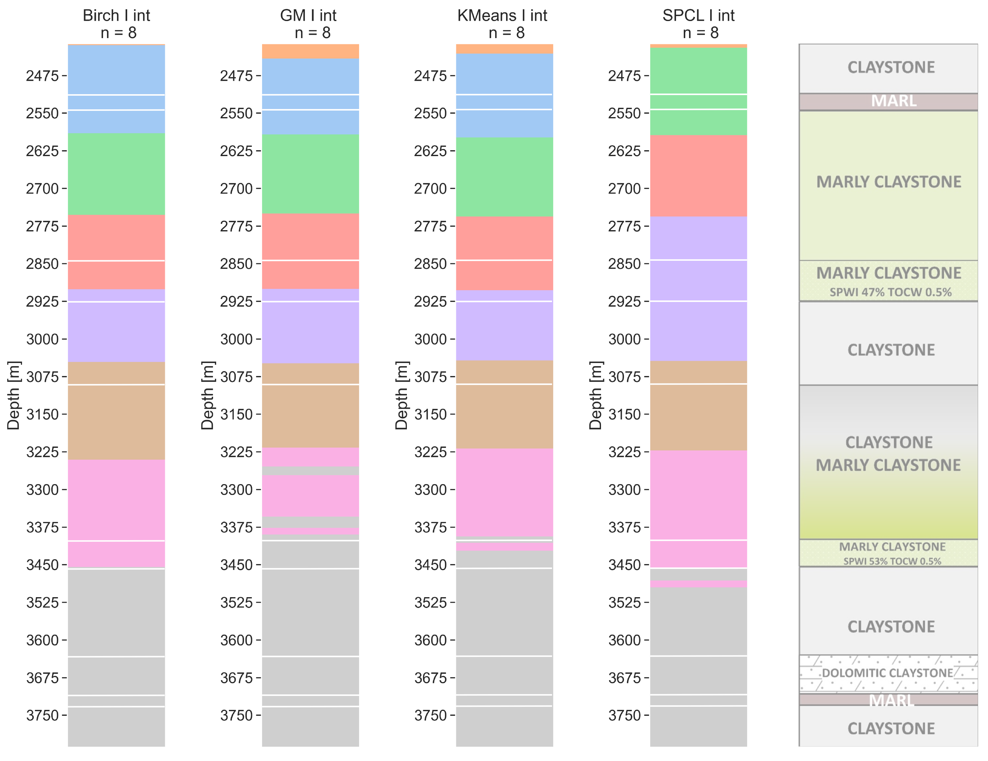
6.2. Eight Clusters
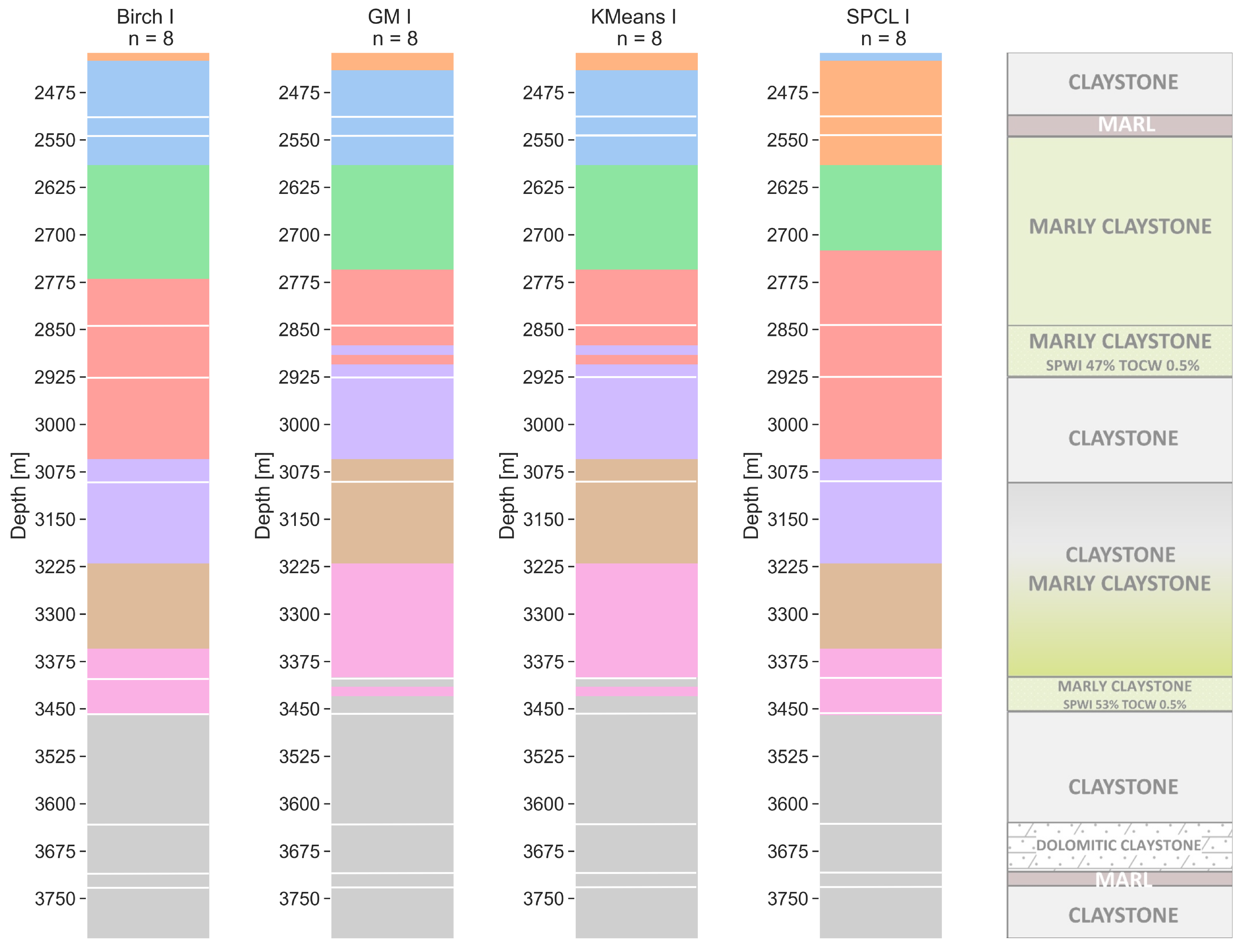
For both resolutions—walkaway VSP (Figure 8) and the sonic one (Figure 9)—consistent models were obtained with small but important differences. The models obtained from the dataset with the walkaway VSP resolution (Figure 8) in general diversify the marly claystone layer in honor of marl and claystone. The thickness of the first three layers is similar for all models. Layers 4 (red) and 7 (pink) show the greatest diversity in terms of thickness. Similar results for these layers are obtained in the pairs of SPCL–BIRCH and GM–k-means. What is important is that the GM and k-means showed clusters within potentially saturated layers (depth of 2900 m MDGL and 3400 m). The sonic resolution models (Figure 9) for BIRCH, GM, and k-means are very consistent. The significant difference begins only at a depth of 3225–3525 m MDGL. The SPCL model is also quite similar to the others; however, a clear division within lithological types is noticeable. For BIRCH, GM, and k-means, the division on marl and claystone in both marly claystone layers is again visible. Only the models from GM and k-means showed a potentially saturated layer, with a depth of around 3400 m MDGL; however, k-means gives slightly more balanced and accurate results here.
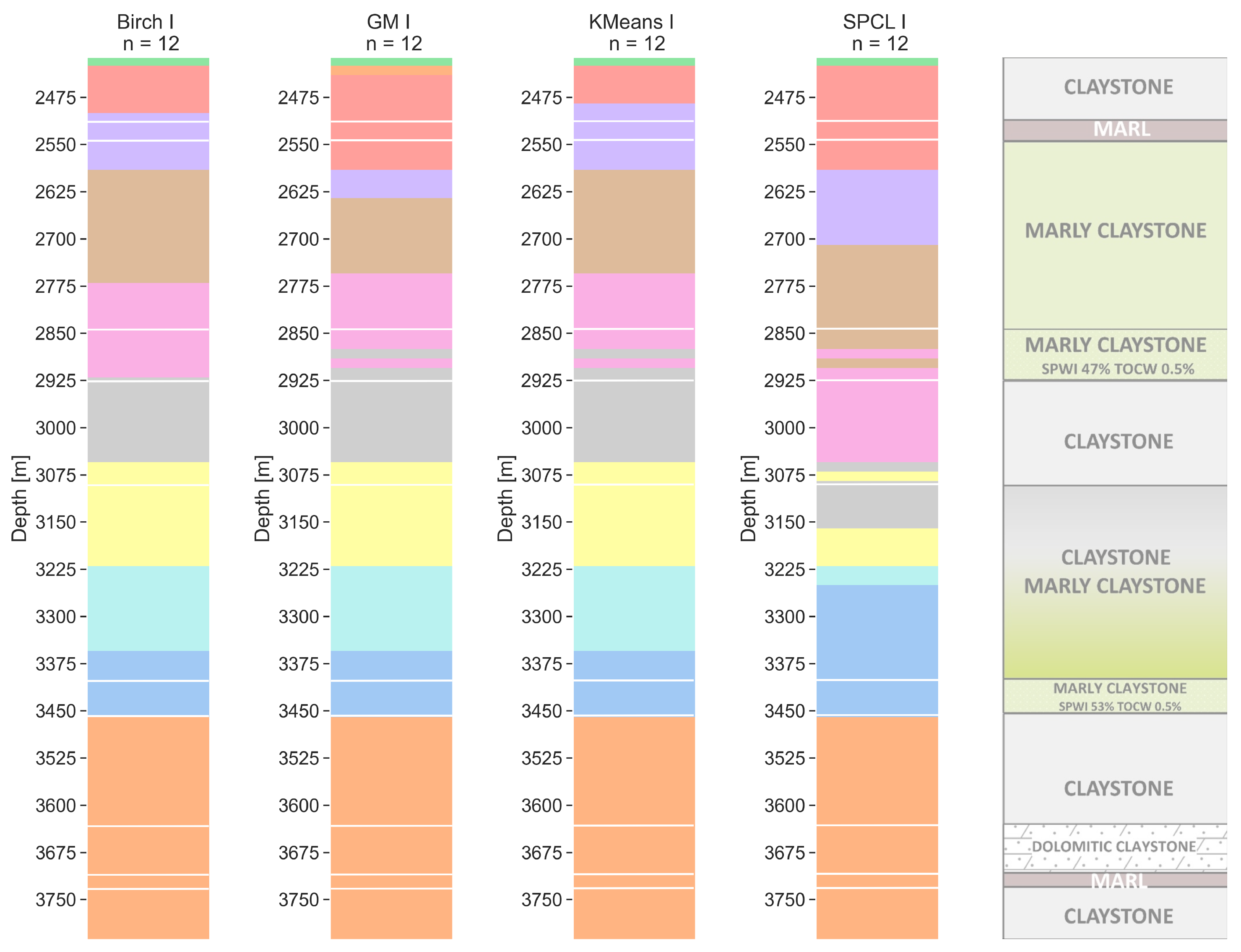
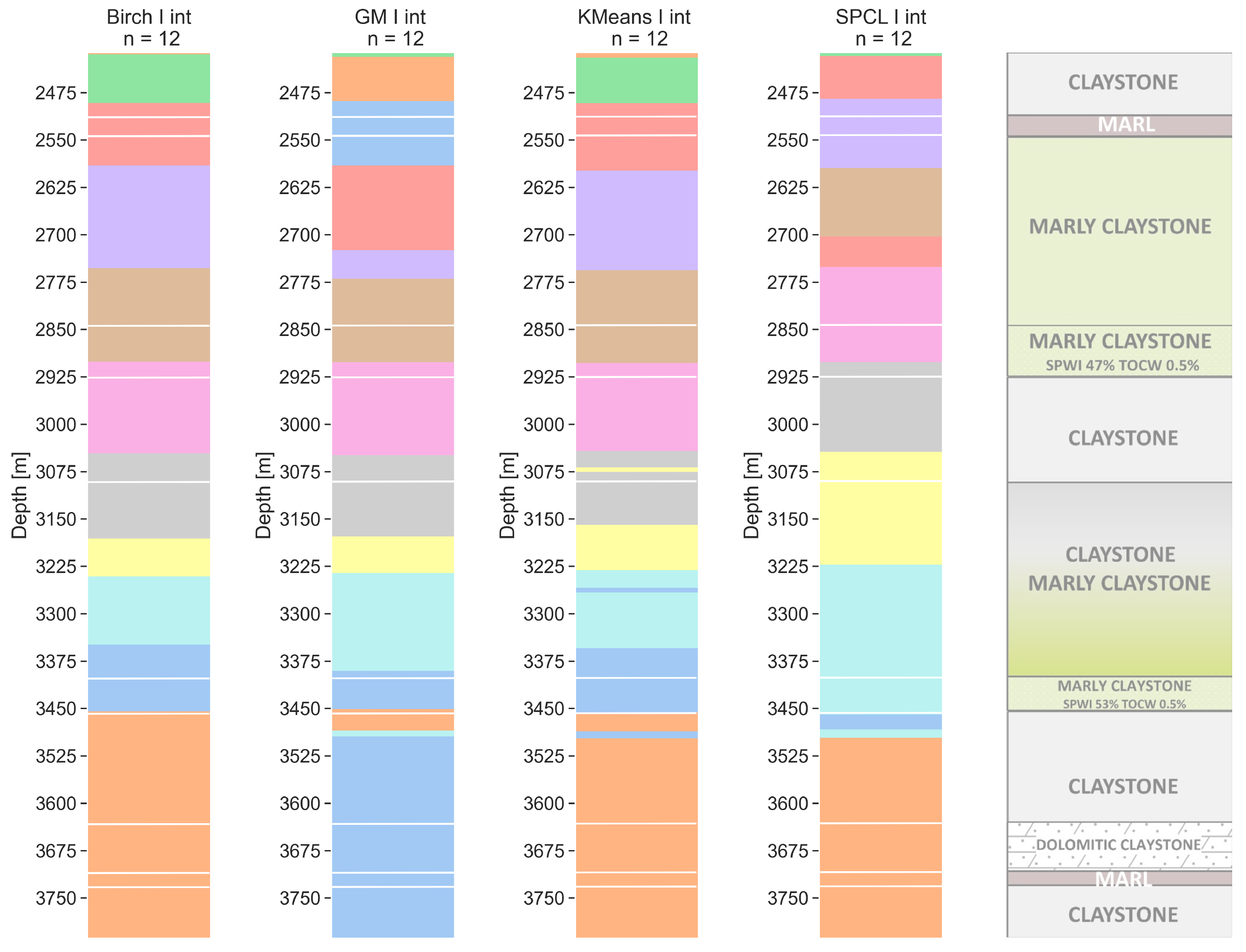
6.3. Twelve Clusters
The number 12 is similar to the number of layers determined from the core analysis in the Silurian complex. For the walkway, the VSP resolution (Figure 10) results are similar to those obtained with n = 8. For all four models, the clusters are quite similar, but the difference for SPCL is again the greatest. For the walkaway VSP resolution, the last cluster for all models starts at a depth of 3450 m MDGL which is the boundary between different Silurian epochs. GM, k-means, and SPCL are sensitive to the thin saturated marly claystone layer (between 2850 and 2925 m MDGL), whereas BIRCH does not divide this layer. The second potentially saturated layer is not properly divided in all models (too thick). For sonic resolution (Figure 11), the models are far less consistent with the walkaway VSP resolution than they were for n = 4 and n = 8; however, there is still a good similarity between them within the sonic measurement step. BIRCH and k-means here are very similar. The model obtained with BIRCH is the most homogeneous, while the k-means show many local thin clusters. SPCL and GM are similar at depths of up to 3075 m MDGL. The internal differentiation of the first marly claystone layer is important here. SPCL shows a thin cluster below the bottom of the second saturated marly claystone, whereas BIRCH and k-means showed that this layer was too thick. On the other hand, the GM model matches with the top and bottom of this layer exactly. Again, in no scenario in terms of resolution and for any model can we see a clusters’ separation for depths greater than 3500 m MDGL.
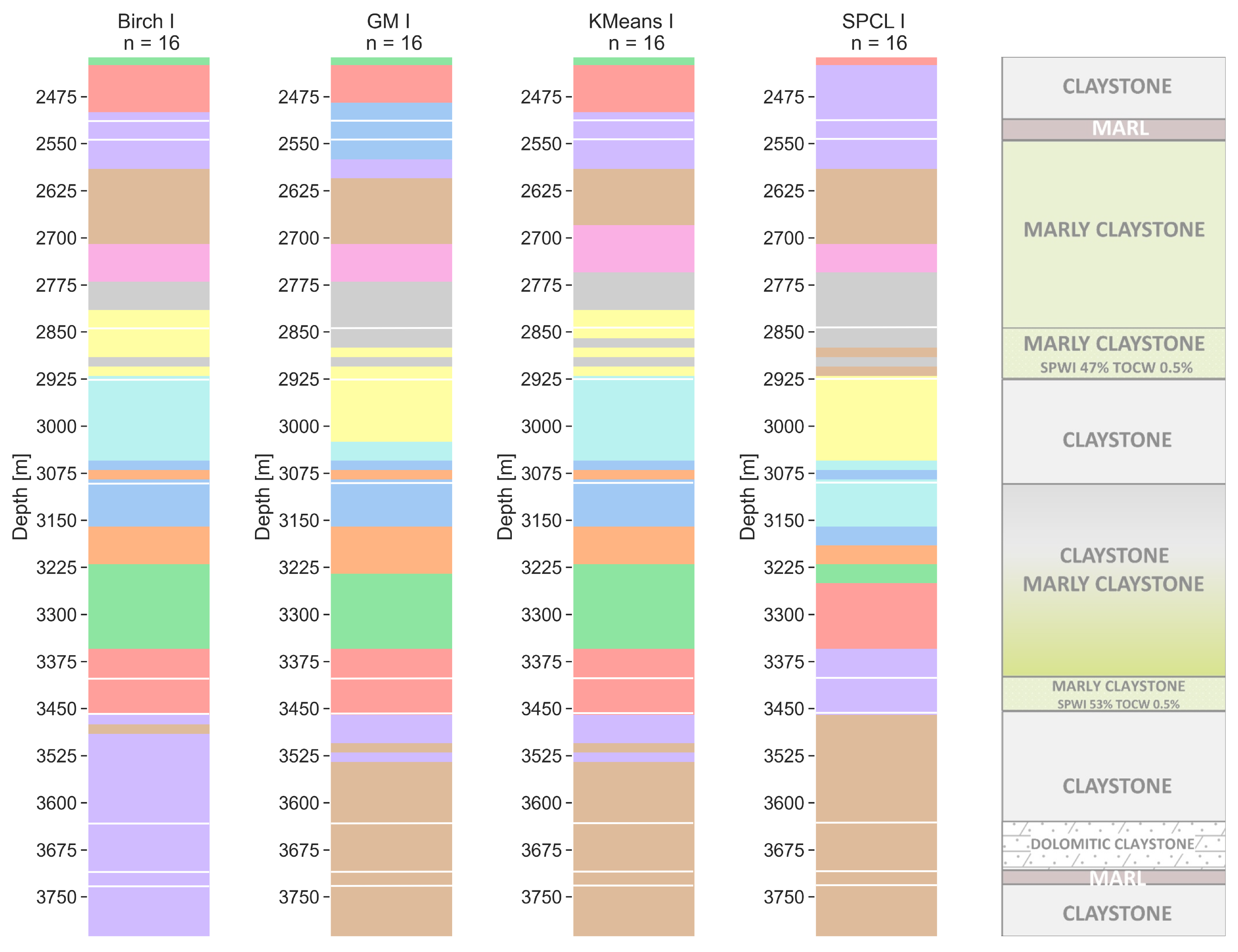
6.4. Sixteen Clusters
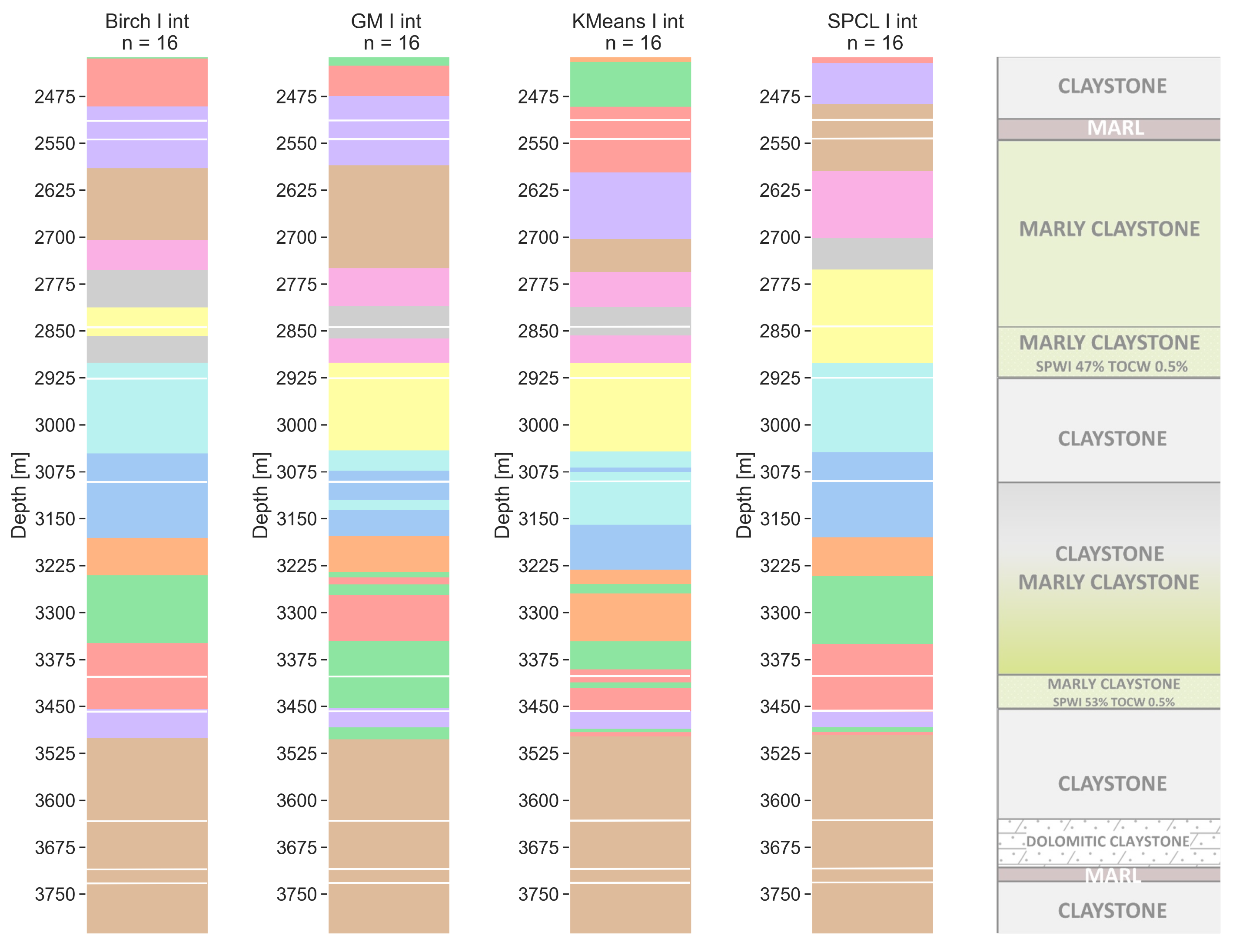
Models for 16 clusters are more difficult to interpret. The differences between walkaway VSP (Figure 12) and sonic (Figure 13) are higher than for n = 4, n = 8, and n = 12. On the other hand, models within a particular resolution are consistent. All four walkaway VSP resolution models show an internal division of the first marly claystone layer, similar to that obtained for the sonic resolution when n = 12. The first layer of saturated marly claystone is divided among all four models; however, the GM, k-means, and SPCL show that this layer can be divided into thinner ones. Very good results (again for all four models) are obtained for the top of the claystone and marly claystone layer (depth of 3075 m MDGL). The walkaway VSP resolution models show that there is no gradual transition from claystone to marly claystone, but this complex has a clear separation layer at a depth of 3150 m MDGL. For all four models, the second saturated marly claystone layer is thicker than that from the core analysis. For GM and k-means, there is a thin cluster at a depth of 3252 m MDGL. For sonic resolution (Figure 13), the GM and k-means models show a significantly greater variation at depths below 3075 m MDGL, whereas BIRCH and SPCL appear to show more major variations. Again, the marly claystone layer shows greater internal differentiation compared to the core analyses, but of a slightly different nature than those obtained for the walkaway VSP resolution. The k-means algorithm shows the best separation of potentially saturated layers, but within the profile from 2400 to 3350 m MDGL, it is almost identical to the model from GM. Neither method shows any differentiation below a depth of 3500 m MDGL, even though, based on the drill core, a thin layer of marl and dolomitic claystone was separated there within two claystone complexes.
7. Discussion
The paper analyzes the possibility of using unsupervised machine learning to detail information on the rock medium with the use of elastic wavefield measurements. Data from the first and experimental acquisition of walkaway VSP in Poland were used. Based on these measurements, detailed in situ anisotropy, polarization, and velocity parameters were obtained. They were an important element of clustering. Measurements in the borehole with a dipole acoustic tool were also used. Consequently, 45 input parameters for clustering were obtained.
Walkaway VSP and sonic measurements are characterized by different resolutions resulting from various source frequencies, ranges, and measurement depth steps. The problem of finding a common data sampling resolution for clustering was one of the challenges of this work. The higher resolution of the well-log measurements provides more information, but, at the same time, it is more affected by noise. The presence of noise negatively affects the results of clustering. On the other hand, a larger data set should produce better results for methods based on probability analysis. Unsupervised machine learning aims to provide new, unknown information about the object, so it is difficult to decide which resolution is better without additional studies.
Another challenge was to determine the optimal number of clusters. This is not an easy task. It is often based on the analysis of the distance between clusters, and the selection of the appropriate minimum or maximum among many local ones is highly subjective. That is why it is important to analyze the obtained model based on domain knowledge and on slightly more objective criteria, such as the BIC, which often produce one global minimum; therefore, the choice is objective.
Using the knowledge of the geology of the region, knowledge from other geophysical surveys, and knowledge of what the main purpose of the study is (improving the velocity model), a detailed analysis of the results was carried out in order to determine the final clustering model. One of the main factors determining the choice of the optimal model was the model’s ability to determine potentially saturated layers.
The models obtained for n = 4 show similarities with each other. Most of the elastic boundaries determined by clustering are at similar depths. A particularly high accuracy is visible for the fourth complex determined by clustering. The most significant differences between the walkaway VSP and sonic models are visible for the third complex. The greater similarity of models was obtained for sonic resolution. The extent of the separated complexes coincides with the main velocity complexes designated for seismic migration. There are also correlations with the main lithological types. None of the tested algorithms were able to identify potentially saturated layers. Therefore, none of the models for n = 4 were selected as the most optimal.
According to the BIC, the number of clusters equal to eight is the most suitable as the initial model parameters. The results are consistent for all clustering methods. The number eight is also optimal in terms of these specific observations. It provides a good balance between over-splitting and provides new information based on the field of elastic waves. For the VSP resolution, a clear similarity between GM and k-means is visible. The SPCL and BIRCH models did not divide the saturated marly layer, which is their disadvantage. With such a number of clusters, methods based on CF-trees and algebraic graph theory seem to tend to over-generalize the model and omit some important details. On the other hand, probabilistic and vector quantization methods successfully distinguished the most significant Silurian intervals. The clusters obtained for data with a higher vertical resolution gave worse results. None of the analyzed algorithms recovered information about the first saturated layer, and, in the case of the second, its position was different depending on the depth. This situation is also reflected in the value of the BIC. For lower-resolution data, the minimum on the curve was visible, whereas this was not the case for for well-log data. Therefore, the GM eight-cluster model in the VSP walkaway resolution is recommended as the most suitable for further work on the velocity model for surface seismic.
The analysis of the metrics for the number of clusters equal to 12 was ambiguous. Unlike the values 4, 8, and 16, some of them (CH and SN) did not indicate this number as optimal. For n = 12, the algorithms did not cope well with the determination of saturated layers, except for the GM, SPCL, and k-means methods for the walkaway VSP resolution (for the first saturated layer). The number of clusters being 12 thus appears to be the least appropriate choice for both sonic and walkaway VSP data resolution.
Sixteen-cluster models for both resolutions and for all tested algorithms give satisfactory results. The separation of saturated layers was mostly obtained. In many places, the boundaries of the layers for different methods coincide, which proves that the models are compatible. However, the models for SPCL exhibit a slightly greater generalization, which may be helpful for typical lithological analyses, whereas the GM and k-means models have much greater detail, which may be useful for borehole geophysics analyses. Models for the VSP resolution seem to work well for the whole depth range. The GM and k-means models for the hole resolution in the lower parts of the Silurian rocks are characterized by greater layer fragmentation.
8. Conclusions
Our research has shown that clustering is a useful tool that allows us to obtain new information about a geological medium using data from walkaway VSP and sonic tool logs. The optimal selection of clusters based on internal metrics is ambiguous. Knowledge about the region and other additional available information allow for a better selection of the optimal number of clusters based on previously predefined numbers (based on statistical metrics). The problem of different research resolutions is important. Depending on whether the parameters will be upscaled or downscaled, different results of clustering will be obtained. Depending on the chosen method, they will be more or less significant. In the context of cluster analysis, for the velocity model correction, the smaller number of clusters and the lower resolution of walkaway VSP tests proved to be more useful. However, in the case of more precise analyses of fine layers, a greater number of clusters and an analysis at a higher sonic measurement resolution seem to be better. The least optimal results were obtained with the BIRCH method. The SPCL method showed a good relationship with the main lithological types and was resistant to local anomalies. The best results were obtained for the GM method when n = 8 and k-means when n = 16.
Author Contributions
Conceptualization, M.Z.; methodology, M.Z.; validation, M.Z., T.D.; formal analysis, M.Z.; investigation, M.Z.; writing—original draft preparation, M.Z.; writing—review and editing, M.Z., T.D., M.S.; visualization, M.Z.; supervision, T.D.; project administration, M.S.; funding acquisition, M.S. All authors have read and agreed to the published version of the manuscript.
Funding
This research was funded by National Center of Research and Development (NCBiR), co-financed by POGC and Orlen Upstream Sp. z o.o. supervised by Department of Fossil Fuels, Faculty of Geology, Geophysics and Environmental Protection AGH UST grant number BG1/GASLUPSEJSM/13.
Institutional Review Board Statement
Not applicable.
Informed Consent Statement
Not applicable.
Data Availability Statement
Not applicable.
Acknowledgments
Data from walkaway VSP measurement were gathered as part of the project: “Seismic surveys and their application for the detection of shale gas zones. Selection of optimal acquisition and processing parameters to map the geological structure and distribution of petrophysical and geomechanical parameters of prospective rocks”, acronym “GASLUPSEJSM”, no. BG1/GASLUPSEJSM/13, a part of Blue Gas I program financed by National Center of Research and Development (NCBiR), co-financed by POGC and Orlen Upstream Sp. z o.o. supervised by Department of Fossil Fuels, Faculty of Geology, Geophysics and Environmental Protection AGH UST, thanks to the efforts of Michal Stefaniuk, Tomasz Mackowski, and Andrzej Pasternacki. We are grateful to POGC for agreeing to use well-log and seismic data acquired as part of the project “Polish technologies for shale gas”.
Conflicts of Interest
The authors declare no conflict of interest.
References
- Tsvankin, I.; Gaiser, G.; Grechka, V.; Baan, M.V.D.; Thomsen, L. Seismic anisotropy in exploration and reservoir characterization: An overview. Geophysics 2010, 75, 75A15. [Google Scholar] [CrossRef] [Green Version]
- Zareba, M.; Danek, T. Nonlinear anisotropic diffusion techniques for seismic signal enhancing—Carpathian Foredeep study. E3S Web Conf. 2018, 66, 1–10. [Google Scholar] [CrossRef]
- Zareba, M.; Danek, T. VSP polarization angles determination: Wysin-1 processing case study. Acta Geophys. 2018, 66, 1047–1062, Erratum in Acta Geophys. 2019, 67, 737. [Google Scholar] [CrossRef]
- Bashir, Y.; Ghosh, D.; Sum, C. Influence of seismic diffraction for high-resolution imaging: Applications in offshore Malaysia. Acta Geophys. 2018, 66, 305–316. [Google Scholar] [CrossRef]
- Zareba, M.; Danek, T.; Zajac, J. On Including Near-surface Zone Anisotropy for Static Corrections Computation-Polish Carpathians 3D Seismic Processing Case Study. Geosciences 2020, 10, 66. [Google Scholar] [CrossRef] [Green Version]
- Zareba, M.; Laskownicka, A.; Zajac, J. The use of S-guided CREP methodology for advanced seismic structure enhancing processing. Acta Geophys. 2019, 67, 1711–1719. [Google Scholar] [CrossRef] [Green Version]
- Michie, D.; Spiegelhalter, D. Machine Learning, Neural and Statistical Classification Ellis Horwood Series in Artificial Intelligence; Prentice Hall: Hoboken, NJ, USA, 1994. [Google Scholar]
- Ayodele, T.O. Introduction to Machine Learning. In New Advances in Machine Learning; Zhang, Y., Ed.; IntechOpen: London, UK, 2010; Chapter 1. [Google Scholar] [CrossRef] [Green Version]
- Zareba, M.; Danek, T.; Stefaniuk, M. P-Wave-Only Inversion of Challenging Walkaway VSP Data for Detailed Estimation of Local Anisotropy and Reservoir Parameters: A Case Study of Seismic Processing in Northern Poland. Energies 2021, 14, 2061. [Google Scholar] [CrossRef]
- Szczypiorska, A. Program Blue Gas—Polski Gaz Łupkowy. 2014. Available online: https://infolupki.pgi.gov.pl/pl/technologie/program-blue-gas-polski-gaz-lupkowy (accessed on 1 June 2022). (In Polish)
- Alkhalifah, T.; Tsvankin, I. Velocity analysis for transversely isotropic media. Geophysics 1995, 60, 1550–1556. [Google Scholar] [CrossRef]
- Thomsen, L. Weak elastic anisotropy. Geophysics 1986, 51, 1954–1966. [Google Scholar] [CrossRef]
- Grechka, V.; Mateeva, A. Inversion of P-wave VSP data for local anisotropy: Theory and case study. Geophysics 2007, 72, 69–79. [Google Scholar] [CrossRef]
- Pedregosa, F.; Varoquaux, G.; Gramfort, A.; Michel, V.; Thirion, B.; Grisel, O.; Blondel, M.; Prettenhofer, P.; Weiss, R.; Dubourg, V.; et al. Scikit-learn: Machine Learning in Python. J. Mach. Learn. Res. 2011, 12, 2825–2830. [Google Scholar]
- Kondracki, J. Regional Geography of Poland; WN PWN: Warszawa, Poland, 2011. [Google Scholar]
- Kasperska, M.; Marzec, P.; Pietsch, P.; Golonka, K. Seismo-geological model of the Baltic Basin (Poland). Ann. Soc. Geol. Pol. 2019, 89, 195–213. [Google Scholar] [CrossRef] [Green Version]
- Domagala, K.; Mackowski, T.; Stefaniuk, M.; Reicher, B. Prediction of Reservoir Parameters of Cambrian Sandstones Using Petrophysical Modelling—Geothermal Potential Study of Polish Mainland Part of the Baltic Basin. Energies 2021, 14, 3942. [Google Scholar] [CrossRef]
- Hamerly, G.; Elkan, C. Alternatives to the k-means algorithm that find better clusterings. In Proceedings of the 2002 ACM CIKM International Conference on Information and Knowledge Management, McLean, VA, USA, 4–9 November 2002; pp. 600–607. [Google Scholar] [CrossRef]
- Hamerly, G. Learning Structure and Concepts in Data through Data Clustering. Ph.D. Thesis, University of California, San Diego, CA, USA, 2003. [Google Scholar]
- Judd, D.; McKinley, P.; Jain, A. Large-scale parallel data clustering. IEEE Trans. Pattern Anal. Mach. Intell. 1998, 20, 871–876. [Google Scholar] [CrossRef] [Green Version]
- Abbas, H.M.; Fahmy, M.M. Classified vector quantization using variance classifier and maximum likelihood clustering. Pattern Recognit. Lett. 1994, 15, 49–55. [Google Scholar] [CrossRef]
- Omran, M.; Engelbrecht, A.; Salman, A.A. An overview of clustering methods. Intell. Data Anal. 2007, 11, 583–605. [Google Scholar] [CrossRef]
- Zhang, T.; Ramakrishna, R.; Livny, M. BIRCH: An Efficient Data Clustering Method for Very Large Databases. SIGMOD Rec. 1996, 25, 103–114. [Google Scholar] [CrossRef]
- Lang, A.; Schubert, E. BETULA: Fast clustering of large data with improved BIRCH CF-Trees. Inf. Syst. 2021, 108, 101918. [Google Scholar] [CrossRef]
- McLachlan, G.J.; Basford, K.E. Mixture Models: Inferenceand Applications to Clustering; Marcel Dekker: New York, NY, USA, 1988. [Google Scholar]
- McLachlan, G.J.; Peel, D. Robust cluster analysis via mixturesof multivariatet-distributions. In Lecture Notes in Computer Science; Amin, A., Dori, D., Pudil, P., Freeman, H., Eds.; Springer: Berlin/Heidelberg, Germany, 1998; Volume 1451, pp. 658–666. [Google Scholar]
- McLachlan, G.J.; Peel, D. Finite Mixture Models; Wiley Series in Probability and Statistics; Wiley: New York, NY, USA, 2000. [Google Scholar]
- Fletcher, R. Practical Methods of Optimization, 2nd ed.; John Wiley and Sons, Ltd.: Hoboken, NJ, USA, 2000. [Google Scholar]
- Nocedal, J.; Wright, S.J. Numerical Optimization; Springer: New York, NY, USA, 1999. [Google Scholar] [CrossRef]
- McLachlan, G.J.; Krishnan, T. The EM Algorithm and Extensions, 2nd ed.; Wiley Series in Probability and Statistics; Wiley: Hoboken, NJ, USA, 2008. [Google Scholar]
- Bishop, C.M. Pattern Recognition and Machine Learning. In Information Science and Statistics; Jordan, M., Kleinberg, J., Scholkopf, B., Eds.; Springer: Cham, Switzerland, 2006. [Google Scholar]
- Lloyd, S. Least squares quantization in PCM. IEEE Trans. Inf. Theory 1982, 28, 129–137. [Google Scholar] [CrossRef] [Green Version]
- Mohiuddin, A.; Seraj, R.; Islam, S.M.S. The k-means Algorithm: A Comprehensive Survey and Performance Evaluation. Electronics 2020, 9, 1295. [Google Scholar] [CrossRef]
- Jia, H.; Ding, S.; Xu, X.; Nie, R. The latest research progress on spectral clustering. Neural Comput. Appl. 2014, 24, 1477–1486. [Google Scholar] [CrossRef]
- Huang, Z. A fast clustering algorithm to cluster very large categorical data sets in data mining. In SIGMOD Workshop on Research Issues on Data Mining and Knowledge Discovery; DMKD: Tucson, AZ, USA, 1997; pp. 146–151. [Google Scholar]
- Ding, S.; Jia, H.; Zhang, L.; Jin, F. Research of semi-supervised spectral clustering algorithm based on pairwise constraints. Neural Comput. Appl. 2014, 24, 211–219. [Google Scholar] [CrossRef]
- Zhang, L.; Hou, L.; Lei, D. Spectral clustering algorithm based on Hadoop cloud platform research and implementation. In Proceedings of the 2016 5th International Conference on Advanced Materials and Computer Science, Qingdao, China, 26–27 March 2016; pp. 495–498. [Google Scholar] [CrossRef] [Green Version]
- Halkidi, M.; Batistakis, Y.; Vazirgiannis, M. On Clustering Validation Techniques. J. Intell. Inf. Syst. 2001, 17, 107–145. [Google Scholar] [CrossRef]
- Banthia, A.; Jayasumana, A.; Malaiya, Y. Data size reduction for clustering-based binning of ICs using principal component analysis (PCA). In Proceedings of the 2005 IEEE International Workshop on Current and Defect Based Testing, Palm Springs, CA, USA, 1 May 2005; pp. 24–30. [Google Scholar] [CrossRef]
- Davies, D.L.; Bouldin, D.W. A Cluster Separation Measure. IEEE Trans. Pattern Anal. Mach. Intell. 1979, PAMI-1, 224–227. [Google Scholar] [CrossRef]
- Caliński, T.; Harabasz, J. A dendrite method for cluster analysis. Commun. Stat 1974, 3, 1–27. [Google Scholar]
- Nielsen, F. Partition-Based Clustering with k-Means. In Introduction to HPC with MPI for Data Science; Springer: Cham, Switzerland, 2016; pp. 163–193. [Google Scholar] [CrossRef]
- Keribin, C. Consistent Estimation of the Order of Mixture Models. Sankhyā Indian J. Stat. Ser. A 2000, 62, 49–66. [Google Scholar]
- Celeux, G.; Fruhwirth-Schnatter, S.; Robert, C. Model Selection for Mixture Models-Perspectives and Strategies. In Handbook of Mixture Analysis; CRC Press: Boca Raton, FL, USA, 2018. [Google Scholar]
- Quinto, B. Unsupervised Learning. In Next-Generation Machine Learning with Spark: Covers XGBoost, LightGBM, Spark NLP, Distributed Deep Learning with Keras, and More; Apress: Berkeley, CA, USA, 2020; pp. 189–244. [Google Scholar] [CrossRef]
- Huang, P.; Yao, P.; Hao, Z.; Peng, H.; Guo, L. Improved Constrained k-Means Algorithm for Clustering with Domain Knowledge. Mathematics 2021, 9, 2390. [Google Scholar] [CrossRef]
- Keribin, C. Characterization of well logs using K-mean cluster analysis. J. Pet. Explor. Prod. Technol. 2020, 10, 2245–2256. [Google Scholar] [CrossRef]
- Churochkin, I.I.; Kharitontseva, P.A.; Roslin, P. Well log clustering as a tool for rock typing of carbonate reservoir. Data Sci. Oil Gas 2020, 2020, 1–5. [Google Scholar] [CrossRef]
- Schlanser, K.; Grana, D.; Campbell-Stone, E. Lithofacies classification in the Marcellus Shale by applying a statistical clustering algorithm to petrophysical and elastic well logs. Interpretation 2016, 4, SE31–SE49. [Google Scholar] [CrossRef]
- Zareba, M.; Danek, T.; Stefaniuk, M. Some statistical consideration of azimuth and inclination angles determination based on walk-away VSP data in Python. E3S Web Conf. 2019, 133, 01006. [Google Scholar] [CrossRef]
- Brie, A.; Endo, T.; Hoyle, D.; Codazzi, D.; Esmersoy, C.; Hsu, K.; Denoo, S. New Directions in Sonic Logging. Oilfield Rev. 1998, 10, 40–55. [Google Scholar]
- Luo, J.; Ying, K.; Bai, J. Savitzky–Golay smoothing and differentiation filter for even number data. Signal Process. 2005, 85, 1429–1434. [Google Scholar] [CrossRef]
Figure 1.
Location of W-1 well (blue rectangle) together with tectonic units and initial velocity model used for seismic depth migration ([9] modified).
Figure 1.
Location of W-1 well (blue rectangle) together with tectonic units and initial velocity model used for seismic depth migration ([9] modified).

Figure 2.
Walkaway VSP measurement.

Figure 3.
Sonic measurement.

Figure 4.
Metrics for cluster number validation for walkaway VSP resolution dataset (inertia analysis—SSE—blue line; silhouette coefficient—SC—green line; Davies–Bouldin index—DB—yellow line; Calinski–Harabasz Index—CH—red line; Bayesian information criterion—BIC—pink line.
Figure 4.
Metrics for cluster number validation for walkaway VSP resolution dataset (inertia analysis—SSE—blue line; silhouette coefficient—SC—green line; Davies–Bouldin index—DB—yellow line; Calinski–Harabasz Index—CH—red line; Bayesian information criterion—BIC—pink line.

Figure 5.
Metrics for cluster number validation for sonic log resolution dataset (inertia analysis—SSE—blue line; silhouette coefficient—SC—green line; Davies–Bouldin index—DB—yellow line; Calinski–Harabasz Index—CH—red line; Bayesian information criterion—BIC—pink line.
Figure 5.
Metrics for cluster number validation for sonic log resolution dataset (inertia analysis—SSE—blue line; silhouette coefficient—SC—green line; Davies–Bouldin index—DB—yellow line; Calinski–Harabasz Index—CH—red line; Bayesian information criterion—BIC—pink line.

Figure 6.
Walkaway VSP resolution clustering models for a number of clusters equal to 4 with lithology from well core (with lines). Clustering methods: BIRCH—balanced iterative reducing and clustering using hierarchies, GM—Gaussian mixture model, k-means, and SPCL—spectral clustering.
Figure 6.
Walkaway VSP resolution clustering models for a number of clusters equal to 4 with lithology from well core (with lines). Clustering methods: BIRCH—balanced iterative reducing and clustering using hierarchies, GM—Gaussian mixture model, k-means, and SPCL—spectral clustering.

Figure 7.
Sonic tool resolution clustering models for a number of clusters equal to 4 with lithology from well core (with lines). Clustering methods: BIRCH—balanced iterative reducing and clustering using hierarchies, GM—Gaussian mixture model, k-means, and SPCL—spectral clustering.
Figure 7.
Sonic tool resolution clustering models for a number of clusters equal to 4 with lithology from well core (with lines). Clustering methods: BIRCH—balanced iterative reducing and clustering using hierarchies, GM—Gaussian mixture model, k-means, and SPCL—spectral clustering.

Figure 8.
Walkaway VSP resolution clustering models for a number of clusters equal to 8 with lithology from well core (with lines). Clustering methods: BIRCH—balanced iterative reducing and clustering using hierarchies, GM—Gaussian mixture model, k-means, and SPCL—spectral clustering.
Figure 8.
Walkaway VSP resolution clustering models for a number of clusters equal to 8 with lithology from well core (with lines). Clustering methods: BIRCH—balanced iterative reducing and clustering using hierarchies, GM—Gaussian mixture model, k-means, and SPCL—spectral clustering.

Figure 9.
Sonic tool resolution clustering models for a number of clusters equal to 8 with lithology from well core (with lines). Clustering methods: BIRCH—balanced iterative reducing and clustering using hierarchies, GM—Gaussian mixture model, k-means, and SPCL—spectral clustering.
Figure 9.
Sonic tool resolution clustering models for a number of clusters equal to 8 with lithology from well core (with lines). Clustering methods: BIRCH—balanced iterative reducing and clustering using hierarchies, GM—Gaussian mixture model, k-means, and SPCL—spectral clustering.

Figure 10.
Walkaway VSP resolution clustering models for a number of clusters equal to 12 with lithology from well core (with lines). Clustering methods: BIRCH—balanced iterative reducing and clustering using hierarchies, GM—Gaussian mixture model, k-means, and SPCL—spectral clustering.
Figure 10.
Walkaway VSP resolution clustering models for a number of clusters equal to 12 with lithology from well core (with lines). Clustering methods: BIRCH—balanced iterative reducing and clustering using hierarchies, GM—Gaussian mixture model, k-means, and SPCL—spectral clustering.

Figure 11.
Sonic tool resolution clustering models for a number of clusters equal to 12 with lithology from well core (with lines). Clustering methods: BIRCH—balanced iterative reducing and clustering using hierarchies, GM—Gaussian mixture model, k-means, and SPCL—spectral clustering.
Figure 11.
Sonic tool resolution clustering models for a number of clusters equal to 12 with lithology from well core (with lines). Clustering methods: BIRCH—balanced iterative reducing and clustering using hierarchies, GM—Gaussian mixture model, k-means, and SPCL—spectral clustering.

Figure 12.
Walkaway VSP resolution clustering models for a number of clusters equal to 16 with lithology from well core (with lines). Clustering methods: BIRCH—balanced iterative reducing and clustering using hierarchies, GM—Gaussian mixture model, k-means, and SPCL—spectral clustering.
Figure 12.
Walkaway VSP resolution clustering models for a number of clusters equal to 16 with lithology from well core (with lines). Clustering methods: BIRCH—balanced iterative reducing and clustering using hierarchies, GM—Gaussian mixture model, k-means, and SPCL—spectral clustering.

Figure 13.
Sonic tool resolution clustering models for a number of clusters equal to 16 with lithology from well core (with lines). Clustering methods: BIRCH—balanced iterative reducing and clustering using hierarchies, GM—Gaussian mixture model, k-means, and SPCL—spectral clustering.
Figure 13.
Sonic tool resolution clustering models for a number of clusters equal to 16 with lithology from well core (with lines). Clustering methods: BIRCH—balanced iterative reducing and clustering using hierarchies, GM—Gaussian mixture model, k-means, and SPCL—spectral clustering.


Table 1.
List of shot points with their offsets and average polarization angles used for clustering.
Table 1.
List of shot points with their offsets and average polarization angles used for clustering.
| SP Number | abs offset [m] | avg incl [deg] |
|---|---|---|
| SP 1010 | 177 | 3.98 |
| SP 1020 | 262 | 5.34 |
| SP 1030 | 347 | 6.27 |
| SP 1040 | 440 | 7.82 |
| SP 1050 | 533 | 8.97 |
| SP 1060 | 630 | 12.09 |
| SP 1070 | 730 | 14.22 |
| SP 1080 | 830 | 15.19 |
| SP 1090 | 930 | 16.67 |
| SP 1100 | 1030 | 16.89 |
| SP 1110 | 1130 | 16.79 |
| SP 1120 | 1231 | 20.04 |
| SP 1130 | 1332 | 22.78 |
| SP 1140 | 1430 | 23.17 |
| SP 1150 | 1530 | 23.19 |
| SP 1160 | 1630 | 24.99 |
| SP 1170 | 1730 | 26.14 |
| SP 1180 | 1835 | 30.92 |
| SP 1190 | 1927 | 34.51 |
| SP 1200 | 2077 | 36.87 |
| SP 1210 | 2280 | 38.11 |
| SP 1220 | 2377 | 40.67 |
| SP 1230 | 2479 | 42.29 |
| SP 1240 | 2479 | 42.29 |
| SP 1250 | 2732 | 43.89 |
| SP 1260 | 3034 | 46.77 |
| SP 1270 | 3232 | 47.76 |
| SP 1280 | 3430 | 49.73 |
| SP 1290 | 3630 | 54.05 |
| SP 1300 | 3830 | 54.02 |
| SP 1310 | 4032 | 58.87 |
Table 2.
Input parameters used for clustering with their measurement range.
| Walkaway VSP Data | Well-Log Data | ||
|---|---|---|---|
| Parameter | Range | Parameter | Range |
| Inclinations—31 different offsets [DEG] | [1.75, 70] | DTSX [us/ft] | [110, 173] |
| [−0.002, 0.0005] | DTSY [us/ft] | [110, 170] | |
| [−0.007, 0.02] | DTP [us/ft] | [63, 86] | |
| from inversion [m/s] | [3600, 4600] | [m/s] | [1743, 2700] |
| from zero-offset [m/s] | [3550, 4580] | [m/s] | [1775, 2800] |
| [m/s] | [3500, 4800] | ||
| [1.5, 2.2] | |||
| [1.7, 2.1] | |||
| PR | [0.25, 0.35] | ||
| [0.01, 0.03] | |||
Disclaimer/Publisher’s Note: The statements, opinions and data contained in all publications are solely those of the individual author(s) and contributor(s) and not of MDPI and/or the editor(s). MDPI and/or the editor(s) disclaim responsibility for any injury to people or property resulting from any ideas, methods, instructions or products referred to in the content. |
© 2023 by the authors. Licensee MDPI, Basel, Switzerland. This article is an open access article distributed under the terms and conditions of the Creative Commons Attribution (CC BY) license (https://creativecommons.org/licenses/by/4.0/).
Share and Cite
MDPI and ACS Style
Zareba, M.; Danek, T.; Stefaniuk, M. Unsupervised Machine Learning Techniques for Improving Reservoir Interpretation Using Walkaway VSP and Sonic Log Data. Energies 2023, 16, 493. https://doi.org/10.3390/en16010493
AMA Style
Zareba M, Danek T, Stefaniuk M. Unsupervised Machine Learning Techniques for Improving Reservoir Interpretation Using Walkaway VSP and Sonic Log Data. Energies. 2023; 16(1):493. https://doi.org/10.3390/en16010493
Chicago/Turabian StyleZareba, Mateusz, Tomasz Danek, and Michal Stefaniuk. 2023. "Unsupervised Machine Learning Techniques for Improving Reservoir Interpretation Using Walkaway VSP and Sonic Log Data" Energies 16, no. 1: 493. https://doi.org/10.3390/en16010493
Note that from the first issue of 2016, this journal uses article numbers instead of page numbers. See further details here.