Phase Space Factors for Double-Beta Decays
 Sabin Stoica1,2*
  Mihail Mirea1,2
- 1International Centre for Advanced Training and Research in Physics, Magurele, Romania
- 2Horia Hulubei National Institute of Physics and Nuclear Engineering, Magurele, Romania
Double-beta decay is presently a very studied process both theoretically and experimentally due to its potential to provide valuable information about important, but still unknown issues related to the neutrino properties and conservation of some symmetries. In the theoretical study of the double-beta decay two key quantities entering the half-life formulas are important, namely the phase space factors embedding the influence of the Coulomb field of the daughter nucleus on the emitted electrons/positrons, and the nuclear matrix elements embedding the nuclear structure effects of the nuclei participating in the decay. Accurate calculation of both of them are needed for good predictions of the double-beta decay half-lives and transitions still unmeasured, and for constraining various beyond Standard Model parameters associated with mechanisms that may contribute to the neutrinoless double-beta decay modes. During time much attention has been paid to the nuclear matrix elements that were considered to bring the largest uncertainties in the computation of the double-beta decay half-lives, while the phase space factors were considered until the recent past to be computed with enough precision. However, newer computation of the phase space factors performed with more precise methods revealed relevant deviations from their values reported previously, especially for heavier nuclei and for positron emitting and electron capture decay modes. In this paper we review the progress made in the computation of the phase space factors for double beta decay. We begin with the non-relativistic approaches, continue with the relativistic approaches which use approximate electron/positron wave functions, and end up with recent, more precise, computations of the phase space factors where exact electron wave functions are obtained from the resolution of a Dirac equation in a Coulomb-type potential and with inclusion of finite nuclear size and screening effects. We report an up-dated and complete list of the phase space factors (PSF) for the following DBD modes: β−β−, β+β+, ECβ+, and ECEC and for transitions to final ground and first excited 2+ and 0+ states of the daughter nuclei. We also make a comparison between different values of the phase space factors found in literature and discuss the differences between these results.
1. Introduction
Nuclear double beta decay (DBD) is the process with the longest lifetime measured so far, by which an even-even nucleus decays naturally into another even-even nucleus with the same atomic mass A but with the electric charge changed by two units. Within the Standard Model (SM) it can occur through several decay modes with lepton number conservation, namely with the emission of two electrons/positrons and two neutrinos/anti-neutrinos. However, theories beyond SM predict that this process may also occur without emission of neutrinos/anti-neutrinos, namely with lepton number violation (LNV) by two units, and these decay modes are generically called neutrinoless double-beta decays. The DBD modes can be classified according to the number and type of the released leptons, and can be divided in two categories:
1) Decays occurring with LNC
1a) Two neutrino double-electron decay (2νβ− β−)
1b) Two neutrino double-positron decay
1c) Two neutrino electron capture (EC) positron emitting decay (2νECβ+)
1d) Two neutrino double electron capture decay (2νECEC)
2) Decays occurring with LNV by two units
2a) Neutrinoless double-electron decay (0νβ− β−)
2b) Neutrinoless double-positron decay (0νβ+ β+)
2c) Neutrinoless electron capture positron emitting decay (0νECβ+)
2d) Neutrinoless double electron capture decay (0νECEC)
The neutrinoless DBD presents particularly a great interest because it can provide us with information about some conservation laws (lepton number, Charge-Parity, Lorentz symmetry) and about fundamental properties of neutrino as their character (Dirac or Majorana), absolute mass and mass hierarchy, number of flavors (are there other neutrino species than the three ones known until present?), etc.
Complete information about the progress in the study of DBD can be obtained from several excellent reviews written during time given. See for examples the Primakoff and Rosen [1], Haxton and Stephenson [2], Doi et al. [3], Tomoda [4], Suhonen and Civitarese [5], Avignone et al. [6], Ejiri [7], Rodejohann [8], Vogel [9], Vergados et al. [10], which, in turn, contain a comprehensive list of other useful references in domain. The theoretical study of DBD implies firstly the derivation of the half-lives for the above mentioned decay modes and transitions to ground (0+) and excited 2+ and 0+ states of the daughter nucleus. In a good approximation the half-life expressions can be written as products of the phase space factors (PSF) embedding the influence of the Coulomb field of the nucleus on the emitted electrons/positrons and the nuclear matrix elements (NME) embedding the nuclear structure effects of the nuclei participating in the decay. In the case of neutrinoless DBD an additional factor related to the specific mechanism that can contribute to the occurrence of these decays enters as well [11–13]:
where and M2ν(0ν) are the phase space factors and matrix elements for the 2ν (0ν) decay modes, me and < m ν > are the electron and effective neutrino masses, gA is the axial vector coupling constant and n denotes one the DBD modes (1–2). For the 2νββ decay mode the nuclear matrix elements are only on the Gamow-Teller type (GT) (are given by the GT operator), while for the 0νββ they are a sum of GT, Fermi (F), and tensor contributions:
The half-life expressions from above are written such as the “nuclear” parts (NME) are dimensionless quantities while the “atomic” parts (PSF) are given in [yr−1] units. Also, it worth to mention that the PSF are quantities which do not depend on gA, while the NME depend on this constant through the (gV/gA) factor. Much attention has been paid over time to the NME calculation, since it was considered to bring the largest uncertainties in the computation of the DBD half-lives. There are several nuclear methods used more often to calculate the NME, including the quasiparticle random phase approximation (QRPA), the interacting shell model, the interacting boson model, the generator coordinate method, and the projected Hartree-Fock Bogolibov model, etc. These uncertainties come mainly from the choice of the model spaces and type of correlations taken into account in calculation. The results and the discrepancies between the NME obtained with these methods and possible sources of uncertainties in calculations have been extensively discussed in the literature. For the interested reader we suggest a number of references that include the most important results [14–31]. The PSF were considered until the recent past to be computed with enough precision. However, newer computation of these PSF performed with more precise methods revealed relevant deviations from the earlier calculations, especially for heavier nuclei and for positron emitting and EC decay modes. Accurate PSF calculations are very needed now in the study of DBD processes where precision measurements of electron spectra and correlation functions are under way, since they may bring useful information, as for example about possible violation of the Lorentz symmetry or about the effective value of the gA constant.
The purpose of this work is to give a review on the PSF calculations for all decay modes and transitions to final ground and first 0+ and 2+ excited states and to give a complete list of the calculated PSF values (however, we except the decay mode 0νECEC that can not occur to the order of approximation that is presently considered in literature). We begin with the presentation of the earliest calculations using non-relativistic approaches and simple expression of the Fermi factors that allows the analytical computation of the PSF. Then, we continue with relativistic approaches, first with those that use approximate analytical expressions of the Fermi factors, and then with more advanced methods where the Coulomb distortion of the electron wave functions are obtained by solving numerically the Dirac equation with inclusion of the finite nuclear size (FNS) and electron screening effects. In the main part of the review we present our recent PSF calculations where the following ingredients are included in addition to other (recent) similar calculations: (i) the use of a Coulomb potential derived from a realistic proton density distribution in nucleus; (ii) development of new routines with improved numerical precision both for solving the Dirac equations and integrating the PSF expressions, and (iii) inclusion in calculation the most recent Qββ values in Wang et al. [32]. Also, we present the first calculations of the PSF values for transitions to final excited states computed with exact Dirac electron functions. Then, comparing different PSF calculations found in literature, performed with relativistic approaches, we find with few exceptions an agreement within 10% between the PSF values calculated with most recent methods and those performed with approximate electron functions for β−β− and β+β+ decays of lighter nuclei. For heavier nuclei and particularly for EC decay modes we got more and larger discrepancies, whose possible sources are discussed as well.
2. Early Approaches of the Phase Space Factors
The phase space factors represent the distortion of the electron plane waves in the Coulomb field of the nucleus. Thus, to compute PSF for DBD modes we need first to obtain the wave functions of the electron(s)/positron(s) emitted or electron(s) captured in the decay, which are distorted by the Coulomb-type potential of the nucleus. In the first derivations of the DBD half-life formulas the electron wave functions were corrected by multiplying them with the so-called Coulomb functions (or Fermi factors) F(Z, ϵ) obtained in a non-relativistic approximation as the square of the ratio of the solution of a Schrödinger equation in a Coulomb potential given by a point charge Z to a plane wave, evaluated at the origin [2]. They are expressed in an analytical form as follows:
where η = ±αZβ, β = p/ϵ, with p = |p| and ϵ the electron momentum and energy. The +(−) signs are taken for outgoing electrons (positrons).
In their calculations of the DBD half-lives, Primakoff and Rosen [1] used an even simpler expression of these factors obtained from Equation (7) by taking β = 1 in the exponent of the above expression. This permits an analytic evaluation of the phase space integrals resulting in suggestive formulas for DBD half-lives, namely proportional to seventh through eleventh powers of the Qββ values. This approximation is an acceptable one, especially for the DBD of nuclei with low Z with emission of two electrons (β−β−) as it was shown Haxton and Stephenson [2]. Then, going to improve the accuracy in estimating the PSF, in the simplest relativistic approach the Fermi factors are given by the square of the ratio of the solution of a Dirac equation in a Coulomb potential given by a point charge Z to a plane wave, evaluated at the nuclear surface [33].
with γ = [1 − (αZ)2]1/2 and R0 the nuclear radius. Further, a better estimation should include the screening and finite nuclear size effects. This can be done by multiplying the Fermi factors of Equation (8) by a factor L0 that can be taken from Behrens and Janecke [34]. For electrons L0 is considered close to unity for the energies and nuclei of interest, so it is not taken into account in these DBD calculations. For positrons screening enhancements at small β can lead to values substantially larger than unity [34]. To see how large can be the relativistic correction we take the ratio of the two Fermi factors [2]:
First, one observes that this expression is invariant to the change η → −η, so one expects relativistic corrections to be similar for electron and positron emitting modes. As it is discussed in Haxton [33], in the limit of small Z this ratio is approaching to unit, thus the non-relativistic correction to the electron/positron wave functions used for computing PSF for light nuclei can be a good approximation. However, when we are dealing with DBD nuclei, the difference between PSF values calculated with non-relativistic and relativistic Fermi factors can be quite large. For example, in the case of 130Te → 130Xe decay the use of non-relativistic Fermi factors instead of relativistic ones leads to underestimation of the DBD half-life by a factor 5 [33], which increases to a factor 200 for the decay 238U → 238Pu. The same expression for the Fermi factors as Equation (8) but in the limit (αZ)2≪1 are used by Suhonen and Civitarese [5] when they show how one calculates the PSF for DBD.
Suhonen and Civitarese have also used these expressions in their DBD calculations presented in their DBD review [5]. Also, Further, Tomoda used another approach in Tomoda [4], obtaining the Fermi factors necessary for PSF computation as combinations of radial solutions of the Dirac equation in spherical coordinates in a Coulomb potential. The electron radial wave functions are expanded in powers of r and the leading constant terms are retained. In this approximation they estimate the error to be , where peff is the “effective” momentum of the leptons at the nuclear surface (peff = 3Zα/2R0 for electrons and peff = k ~ 1MeV for neutrinos). The radial functions are determined by boundary conditions, namely they have to be finite at r = 0 and become a plane wave plus an incoming spherical wave at infinity. Doi et al. also consider analytical (approximate) Fermi factors in their papers [3, 35–37], with similar expressions as those from Equation (8), but also, without inclusion of the screening effects.
3. Recent Approaches
Kotila and Iachello recalculated the PSF by using exact solutions of the relativistic Dirac equation for Coulomb fields modified by the screening effect [11, 12]. The radial electron/positron wave function were calculated numerically by using the subroutines package RADIAL [38]. The input in the package is the potential V which is primarily the Coulomb potential of the daughter nucleus with charge Zd, V(r) = −Zd(αℏc)/r. The FNS effect is taken into account with a Coulomb potential given by an uniform charge distribution in a sphere of radius with r0 = 1.2 fm [11, 37]:
The screening effect was taken into account by multiplying the above expression of V(r) with a function ϕ(r), solution of the Thomas Fermi equation. The procedure will be described later. This more rigorous relativistic treatment, with the inclusion of FNS and screening effects was also adopted by us in Stoica and Mirea [13],Mirea [39], but with the following improvements: (i) the use of a Coulomb-type potential, obtained from a realistic distribution of the protons in the nucleus, (ii) building up new, more precise and under control, routines; (iii) using more recent Qββ values. In the following, we review our works from Stoica and Mirea [13] and Mirea [39].
4. Theoretical Treatment
The first step in the calculation of the PSF is the determination of the wave function of the electron in the Coulomb field of the nucleus.
4.1. Electron Radial Functions
For free states we use relativistic scattering electron/positron wave functions, solutions of the Dirac equation in a central (Coulomb) potential:
for β− decay and
for β+ decay where κ = (l − j)(2j+1) is the relativistic quantum number and are spherical spinors. The quantities gκ(ϵ, r) and fκ(ϵ, r) are the large and small components of the radial wave functions which satisfy the radial equations:
where V can be negative/positive (for β−/β+). For the continuum spectrum, these functions are normalized so that they have the asymptotic behavior of the Coulomb wave functions:
Here c is the light velocity, me/ϵ are the electron mass/energy, is the electron wave number, , is the asymptotic Sommerfeld parameter, δκ is the global phase shift and V is the Coulomb interaction energy between the electron and the daughter nucleus. For pure Coulomb fields (no screening), the effective charge number is Zeff = ±Z for β∓ decays. The energy is .
The phase shifts are obtained by matching the inner numerical solution to the analytic function. The global phase shift δ = δC + δk [37] is obtained by renormalizing the numerical solution of the Dirac equation in the asymptotic region. The global phase shift depends on the electron energy. It should be taken into consideration when the electron phase factors are calculated [40]. It includes the Coulomb phase shift , with , ζ = ±Zeffα, and the shift due to distorsion of the Coulomb potential δk [38, 41]. The phase shift due to the distorsion of the Coulomb potential is calculated numerically during the renormalization of the numerical solutions to a sinusoidal form given by the Equation (18). The normalization procedure is described in Salvat [38] and Salvat and Mayol [42].
The bound states wave functions for the electron
are solutions of the Dirac equation (17) and correspond to the eigenvalues ϵn (n is the radial quantum number). The quantum number κ is related to the total angular momentum jκ = ∣κ∣−1/2. For simplicity, the quantities and are used in the following. These wave functions are normalized such that
An asymptotic solution is obtained by means of the WKB approximation and by considering that the potential V is negligible small:
where
with
In our calculations we use n=0 and n=1 number of nodes, for the orbitals 1s1/2 and 2s1/2, κ being -1. The eigenvalues of the discrete spectrum are obtained by matching two numerical solutions of the Dirac equation: the inverse solution that starts from the asymptotic conditions and the direct one that starts at r=0.
4.2. The Coulomb Potential
The influence of the nuclear structure was taken into consideration in Stoica and Mirea [13], Mirea [39]. by using a potential V(r) derived from a realistic proton density distribution in the nucleus. This proton density in the nucleus is obtained by solving the Schrödinger equation for a Woods-Saxon potential. In this case the potential becomes:
where the charge density is
Ψi is the proton (Woods-Saxon) wave function of the spherical single particle state i and vi is its occupation amplitude. The factor (2ji + 1) reflects the spin degeneracy.
As an example, the difference between the behavior of the constant charge density ρe and the realistic charge density is displayed in Figure 1 for the daughter nucleus 150Nd. We computed the Coulomb potential with formula (24). In this case, the differences given by the charge densities are translated in a shift of 0.5 MeV energy in the potential at r = 0, as it can be observed in Figure 2. This difference in energy vanishes when r increases, but is able to affect the values of the wave functions.
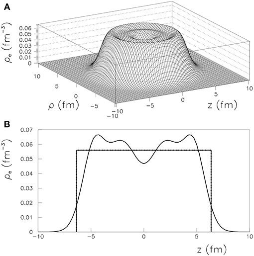
Figure 1. (A) Realistic proton density ρe for 150Nd represented in cylindrical coordinates ρ and z. (B) Profile of the realistic proton density ρe for 150Nd (thick line) compared with that given with the constant density approximation (dot-dashed line).
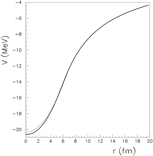
Figure 2. The Coulomb potential V obtained by using the realistic charge density is plotted with a thick full line as function of the radius r. The Coulomb potential obtained with the finite nuclear size approximation is displayed with a thin line. The calculations were performed for the 150Nd.
The Coulomb field felt by the β particle is damped by the electron cloud. A simple way to take into account the screening effect is to multiply the potential V(r) with an universal screening function ϕ(r), which is the solution of the Thomas Fermi equation:
with x = r/b, and a0 = Bohr radius. A solution of this equation having the boundaries conditions ϕ(0) = 1 and ϕ(∞) = 0 was calculated within the Majorana method in Esposito [43]. A solution of the Thomas-Fermi equation was also used Kotila and Iachello [11] to take into account the screening effect. The Equation (26) does not depend on physical constants or on the charge of the parent nucleus, being an universal equation. The condition ϕ(0) = 1 means that the Coulomb potential is not perturbed by the electron cloud in the nuclear region. Asymptotically, ϕ(∞) = 0 means that the Coulomb field has completely disappeared. Therefore, the modality in which the universal screening function modifies the Coulomb potential should be adapted to the boundary conditions related to our specific mechanisms. For example, in the case of the β−β− decay, the asymptotic boundary condition should be , Zd = Z0−2 being the charge number of the daughter. That is, the Coulomb field is suppressed by the screening such that an interaction between β−-particles and an positive ion of charge 2+ is obtained asymptotically. Therefore, we use different methods to introduce the screening accordingly to the universal function ϕ(x).
In the case of the β−β− process, the potential used to obtain the electron wave functions is:
to take into account the fact that DBD releases a final positive ion with charge +2. V(Z, r) is negative. In the relations related to screening we use the atomic units, that is, the product αℏc=1. The asymptotic potential between an electron and a double ionized atom is . In this case, the charge number Z = Z0+2 corresponds to the daughter nucleus, Z0 being the charge number of the parent nucleus. In the case of the β+β+ process, the potential used to obtain the positron wave functions is:
where the final configuration is characterized by an ion with charge -2. V(Z, r) is positive. In this case, the daughter nucleus has the charge number Z = Z0 − 2. In both approaches, at r = 0 the potential is unscreened because ϕ(0) = 1. Asymptotically ϕ(r) tends to 0 and we are left with the charge number of the final system. In the ECβ+ reaction, a simultaneous combination of two processes is inferred. In the case of the EC process, the potential used to obtain the electron wave functions reads:
and the charge number Z = Z0 corresponds to the parent nucleus. V(Z, r) is negative. In the case of the β+ process, the potential used to obtain the positron wave functions reads:
to take into account that in the final configuration we have an ion with charge −1. V(Z, r) is positive. In this case the daughter nucleus has the charge number Z = Z0 − 1. In the case of the ECEC process, the potential used to obtain the electron wave function is:
and Z = Z0, the final system being neutral. In Figure 3, the effective screening ϕeff given by the ratios , , , VEC(x)/V(x) and VECEC(x)/V(x). The behavior of our effective screenings agree to that obtained in Kotila and Iachello [11] where the Thomas-Fermi equation was solved for different boundaries.
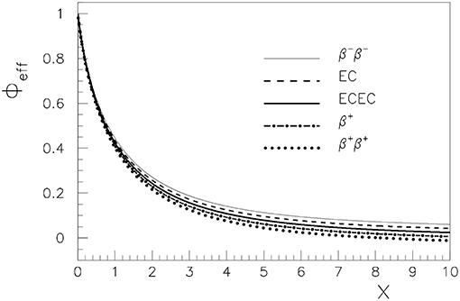
Figure 3. The effective screening function ϕeff as function of the dimensionless parameter x calculated for the 136Xe parent nucleus. The thin full line corresponds to the β−β− decay, the thick dashed line is for the EC process, the thick full line is for the ECEC process, the dot-dashed thick line is for the β+ process and the dotted thick line is for the β+β+ decay.
4.3. Phase Space Factors Formulas
As given in Primakoff and Rosen [1], Doi et al. [44], Haxton et al. [33], and Tomoda [4], the differential ββ decay rate for 0+ → 0+ transitions reads:
where θ12 is the angle between the electrons. Both parameters a0 and a1 represents summation over intermediate nuclear states of products between electron phase factors and nuclear matrix elements summed over intermediate states N
Here, represent the electron phase factors and the matrix elements between initial (I) and final (F) states are denoted
Also,
with . The previous expression depends on the electron energies ϵ1, ϵ2, electron momenta p1, p2 and on the neutrino energies ω1, ω2. Usual values of the parameters can be considered as G = 1.16637 × 10⁻⁵ GeV−2 (the Fermi coupling constant), cos θC=0.9737 (θC standing for the Cabbido-Kobayashi-Maskawa mixing angle between d and s quarks) and gA ≈1 (the axial vector form factor).
By considering that the excitations energies are of the order of giant Gamow-Teller resonance à = 1.12A1/2 MeV, the closure approximation is adopted. That is, the energy of the intermediate state EN is replaced with an average value 〈EN〉. Therefore the energy denominators
are changed within averaged values
In this way, a factorization of the Equation (32) can be realized. By considering and the nuclear matrix element on the form
the half-live obtained with Equation (32) can be written as a product between phase space factors an nuclear matrix elements. By integrating Equation (32), two phase space factors are obtained [4, 11]:
that correspond to the two parameters a(0) and a(1) of Equation (32). An energy dependent angular correlation α is defined as
from
In this work, we report normalized phase factors, in units yr−1. We mention that by this renormalization the quantities G(i) do not depend on the axial-vector constant gA. Also, as one can see from the formulas, the PSF ( depend very little to the average energy < EN >, because this constant enters both to the nominator and denominator in all the PSF expressions.
4.3.1. Double Electron and Double Positron Decay Modes
Here, the electron phase factors are
and
with the products
The values of the f and g functions are approximated with the solutions at the nuclear surface (the method I from [11]).
where fm is the nuclear radius. For the 2νββ decay mode and transitions to ground states (g.s.), the PSF expression reads:
where is the kinetic energy released in the process. 〈KN〉, 〈LN〉 are expressions that depend on the electron/positron (ϵ1,2) and neutrino (ω1,2) energies, and on the g.s. energy of the parent nucleus and on the excited states energy of the intermediate nucleus [2, 3, 5, 11, 35, 36].
Here, the difference in energy in the denominator can be obtained from the approximation , where the empirical systematics à = 1.12A1/2 (in MeV) [2] gives approximately the energy of the giant Gamow-Teller resonance in the intermediate nucleus [11]. The quantity W0 is related to the Qββ value of the process and
where ω1 and are the neutrino energies. The PSF are finally renormalized to the electron rest energy and are reported in [yr−1].
The PSF for the 2νββ decay mode and transitions to excited states is calculated with a formula similar to (52), but replacing Qββ by , which is the kinetic energy released in this transition. is the energy of the excited state of the daughter nucleus x.
For the 2νββ decay mode and transitions to excited state, the PSF formula reads [5, 11–13, 39]:
where .
For the 0νββ decay and transitions to g.s. the PSF reads:
where
For transitions on the 2 state, instead of in Equation (57), the next expression is integrated
In Equations (52, 56, 57), it is convenient to redefine the PSF by a renormalization that eliminates the constant gA and correlates (by dividing by ) the dimension of G0ν with the NME which are dimensionless. These are reflected in the lifetimes formulas (9). Thus, the PSF are also reported in [yr−1]. A similar expression is employed in the PSF calculation for the transitions to excited states, but replacing Qββ by . The formula used for the PSF computation for 2νβ+β+ decay mode is similar to that used for 2νβ−β− decay, but ϵ1,2 are now the positron energies. Also, we use the same approximations as described above, to evaluate the radial positron wave functions (g and f) at the nuclear surface and replace the excitation energy EN in the intermediate odd-odd nucleus by a suitable average energy.
4.3.2. The ECβ+ Case
For the ECβ+ decays the energy released in the process is . If the numerical solutions of the Dirac equation are obtained in Bohr units a0, the probability that an electron is found on the surface of a nucleus of radius RA can be defined as:
The PSF expression for 2νECβ decay mode is
where ϵn, κ are the binding energies of the electron while pp and ϵp are the linear momentum and the energy of the positron. Here, the expressions for 〈KN〉 and 〈LN〉 are similar to those from Equations (53)–(54), but where ϵ1 is replaced by , the energy of the captured electron and ϵ2 is replaced by ϵp, the energy of the emitted positron. For the 0νECβ decay process the PSF expression is:
where ϵp, i denotes the maximal value of the positron associated to the state i.
4.3.3. The 2νECEC Case
The PSF expression is defined as:
where is the energy released in the process. The expressions for 〈KN〉 and 〈LN〉 are similar to those from Equations (53)–(54), but where ϵ(1, 2) are replaced by , the energies of the captured electrons.
5. Numerical Details
The numerical solutions of the Dirac equation are based on the Buhring method [45] which considers a power series expansion of the radial wave functions. Essentially, the numerical algorithm of our code follows the lines given in Salvat and Mayol [42] and Salvat et al. [38]. In such a calculation, the uncertainties are introduced by the interpolation procedure which determine potential values and by the round-off errors. A very dense grid of potential values was taken into account in order to increase the accuracy. The finite size and the screening effects modify the phase shifts. These phase shifts are obtained through a normalization of the free wave functions as explained in Salvat et al. [38, 41].
For bound and free states wave functions, the potential energy corrected with the screening function is calculated in different mesh points defined by an increment x along the distance r. Further, the potential is approximated with a spline cubic function. As mentioned, the radial wave function is expanded as an infinite power series. Successive numerical values of the radial wave function depend on the increment and the coefficients of the spline function by mean of recurrence relations. At r = 0, the solution is determined from the regularity condition. The wave functions are determined step by step in the mesh points. If the round-off errors are considered negligible, the numerical precision depends mainly on the number of terms in the series expansion and on the value of the increment. An increment interval of 10−4 fm and at least 100 terms in the series expansion were considered in our numerical code, exceeding the convergence criteria given Salvat and Mayol [42]. At very large distances, the behavior of the free wave functions determined numerically must resemble to that of the asymptotic Coulomb function, characterized by a value of the Sommerfeld parameter modified by the screening effect. By comparing the behavior of the numerical and the analytical asymptotic solutions, a renormalization to unity and a determination of the phase shift is obtained. For discrete states, the potential provides the boundaries of the solutions. The initial conditions of the reverse solution of the wave function is determined by the WKB approximation. The direct and the reverse wave functions are calculated numerically for different electron energies. The eigenvalue is obtained when the direct solutions and the inverse ones match together. In order to find the bound states of the electron we spanned a range 0.3 MeV smaller than in steps of 0.0002 MeV. The bound solutions of interest are found in this interval.
Concerning the PSF evaluations, it should be noted that all integrals were performed accurately with Gauss-Legendre quadrature in 32 points. Up to 49 values of the radial wave functions on the surface of the nucleus were determined in the Qββ-value interval. The electron phase spaces are obtained by spline interpolations of the values calculated for the electron wave functions. Recently reported Qββ in Wang et al. [32] are used.
6. Results and Discussions
6.1. Phase Space Factors
The PSF values reported in the literature within different models are presented in Tables 1–7. As we mentioned, the PSF values reported by KI in Kotila and Iachello [11], Kotila and Iachello [12], Stoica and Mirea [13] are obtained with a similar approach as ours, namely, the use of exact electron wave functions obtained by solving numerically the Dirac equation and with inclusion of the finite nuclear size and electron screening effects. The results reported in Doi et al. [37], Doi et al. [3], Doi and Kotani [35], and Suhonen and Civitarese [5] are obtained by approximating the electron wave functions at the nuclear surface and without inclusion of the screening effect.
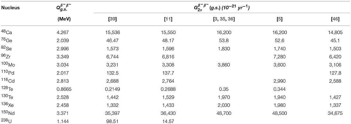
Table 1. PSF for 2νβ−β− decays to final g.s.
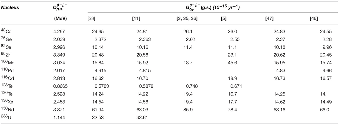
Table 2. PSF for 0νβ−β− decays to final g.s.
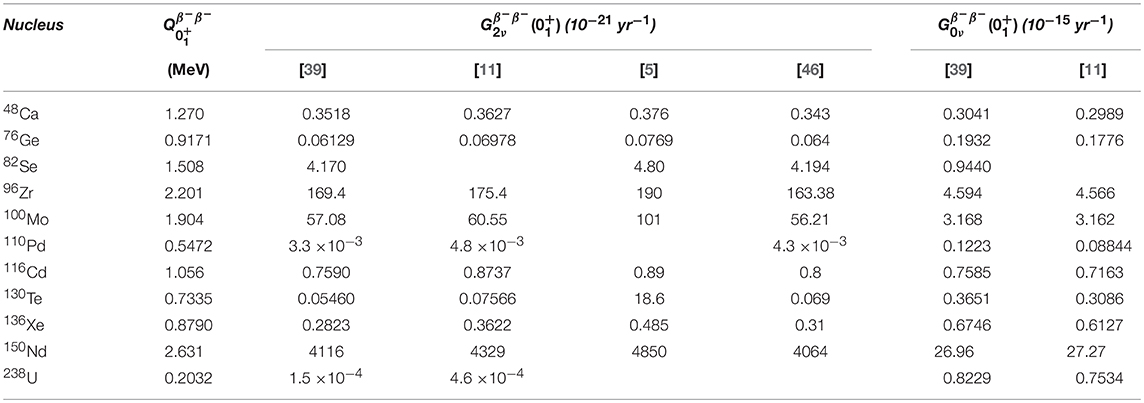
Table 3. PSF for β−β− decays to final excited 0 states.
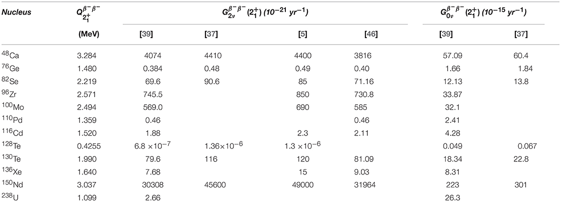
Table 4. PSF for β−β− decays to final excited 2 states.
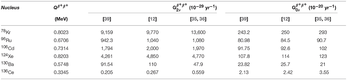
Table 5. PSF for β+β+ decay mode.
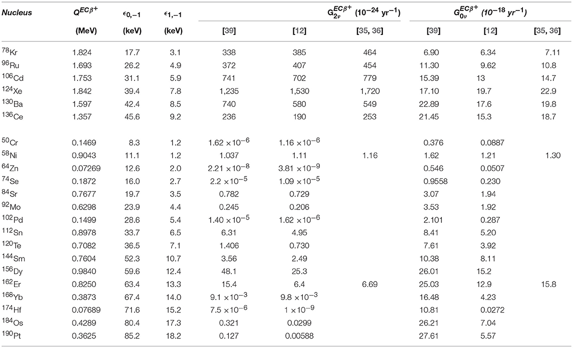
Table 6. PSF for ECβ+ decay mode.
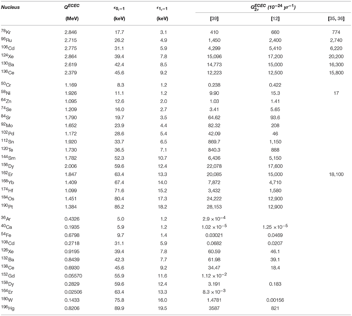
Table 7. PSF for 2νECEC decay mode.
The PSF values for the β+β+ decays are displayed in Table 5. Differences of about 11–30% between G2ν values of Neacsu and Horoi [11] and Mirea et al. [39] are retrieved, in majority of cases. The agreement concerning the G0ν values is very good with one exception: in the case of the 136Ce nucleus, a difference of 13% is found. The differences betweenthe recent PSF values calculated exactly and those reported in Doi and Kotani [35] are larger for most of the results.
The results for ECβ+ decay mode are shown in Table 6 and they are grouped in two sectors: the first sector includes the six nuclei that can also undergo a β+β+ decay and the second one includes the other nuclei which can undergo only ECβ+ decays. One can see that the differences between KI results and ours are relevant in many cases. For the nuclei from the first sector (the most interesting experimentally cases, having the largest QECβ values), we got several PSF values which differ by more than 20% compared to those reported by KI and other authors. For the “pure” ECβ+ decays, we got even more significant differences in several cases as compared with KI results, while other (older) results reported are a few.
The PSF values (G2ν, G0ν) for β−β− decays are presented in Tables 1–4 for transitions to g.s and excited and states, respectively. For the transitions to g.s. (Tables 1, 2) the results reported in Kotila and Iachello [11, 12] are in very good agreement. Apart two exceptions, the differences between the two set of results do not exceed 5%. In the case of nucleus 128Te the difference betwee the G2ν values amounts to 22%. In the case of the 238U nucleus the difference is of about 7 times. We double checked our calculations for this nucleus and did not found errors. For the transitions to excited states (Table 3), there are several cases, especially for heavier nuclei (76Ge, 110Pd, 116Cd, 130Te, 136Xe) with notable differences between the two sets of results, ranging in the interval (10–40)%. The difference for the G2ν in the case of 238U is the largest one. The comparison between the recent results and those previously reported in Doi et al. [37], Doi et al.[3], and Suhonen and Civitarese [5] reveal also larger discrepancies in several cases. For the transitions to excited states (Table 4) recent results are reported in Neacsu and Horoi [46], by using an effective screening method, and with approximate wave functions. Comparing our PSF values for final states with those reported in Doi et al. [37] and Suhonen and Civitarese [5], one observes that the differences range in a 30% interval, both for G0ν and G2ν. A much better agreement is obtained between the data of Neacsu and Horoi [46] and Mirea et al. [39]. It is worth to mention that, although they are not yet measured, the β−β− decays to excited states are of interest to probe alternative mechanisms for occurrence of the 0ν-decay mode, to the (most common) mechanism of exchange of light left-handed neutrinos between two nucleons inside the nucleus.
For the 2νECEC decay mode, the PSF values are given in Table 7. Three groups of nuclei are considered. The first sector includes six nuclei that can also undergo a β+β+ decay. In the second sector, nuclei that can also undergo ECβ+ decays are enumerated. The third sector includes the nuclei which can undergo only 2νECEC decays. The differences between the G2ν values of the recent calculations reported in Kotila and Iachello [11] and Mirea et al. [39] concerning the nuclei from the first sector are within (30-55)%. In the remaining two sectors, the discrepancies are even larger. These differences between the PSF values that are obtained with similar approaches on the one side, and with other approximations on the other side, might be explained by the use of less rigorous approaches, i.e., of approximate electron wave functions, non-inclusion of the screening effect, (possible) less efficient routines at that time, etc.
The differences between results obtained with exact solutions of the Dirac equation [11, 39] may arise from the additional ingredients used in the latter calculation. For example, we got relevant differences between their results and ours especially for decays where the Qββ values are small. For small interval for energy integration, the numerical precision of the PSF expressions depend on values of the free electron wave functions for energies close to where the solutions of the Dirac equation diverges. These situations should be treated carefully. A large number of mesh points in the numerical integration over Qββ values is needed, especially at energies close to the electron mass, in order to get stable results. The calculations performed in Mirea et al. [39] are realized with up to 49 interpolation points. The authors of Mirea et al. [39] observed that after 40 interpolation points the results show no variation. Around the zero kinetic energy of the released electron/positron, an interval energy of about 10−4 MeV was used, because in this region a sudden variation of the wave function amplitude is produced. The use of a Coulomb potential constructed from the density of protons can also contribute to differences of a few percents, especially for EC decays. The use of different reported Qββ values may also contribute to the observed differences up to 3% as remarked in Mirea et al. [39], were the tables of Wang et al. [32] were used. In the cases involving bound electron states, important is the numerical accuracy in the identification of electron/positron bound state 1s1/2 that intervene in the Equation (62). A different procedure was built in Mirea et al. [39] to get the correct electron/positron bound states. The mentioned possible sources of uncertainties can act cumulatively to determine differences between the results obtained by solving numerically the Dirac equation. In our opinion, differences larger that 10% between the values of different PSF computations are important for precise DBD calculations/estimations, hence the evaluation of the PSF for DBD is still a challenge.
6.2. Energy and Angular Distributions
From the DBD decay rates formulas for the energy and angular distributions of the two electrons/positrons released in the decay can also be derived. The normalized energy distributions , and the angular correlation parameter α are calculated for a series of nuclei of interest and are plotted with a thick full line in Figures 4–6 for β−β− decay. The range of energies span the Qββ-value for each investigated nucleus. We also performed calculations without considering the screening effect. The distributions without screening were plotted with a thin full line. Moreover, a calculation of the angular correlation parameter α is realized by considering that the global phase shift is zero and it is plotted with a dashed thin line. The effect of the screening becomes more pronounced for heavier nuclei, as for 136Xe nucleus. Due to the screening, the values of the differential distributions decrease with few percents. The screening is also responsible for a small attenuation of the angular distribution α at energies close to the Qββ-value. A similar behavior was also remarked in Kotila and Iachello [11]. If the global phase shift is set to zero, the absolute values of the angular correlation α become larger. Our results can be compared with single-electron, summed energy spectra and angular correlation spectra provided in Kotila and Iachello [11] for the parent nuclei 136Xe, 82Se, and 150Nd. The behavior of the differential decay rates exhibited by the results given Kotila and Iachello [11] agree with our data, but differ in magnitude. In general, the differential decay rates reported here are larger than those obtained in Kotila and Iachello [11] with about 10%. Also, the α parameter calculated by disregarding the global phase shift in this work seems to agree better with the results published in Kotila and Iachello [11]. New calculations concerning the energy distributions were recently reported in Simkovic et al. [48], where modifications of the shape of the energy distributions were evidenced.

Figure 4. The normalized energy distributions , and the angular correlation parameter α as function of the electron energies ϵ1 and ϵ2 for 82Se parent nucleus β−β− decay are plotted with a full thick line. The results obtained by neglecting the screening effect are plotted with a full thin line. A thin dashed line is used for calculations in which the global phase shift of the Dirac wave functions is set to zero.
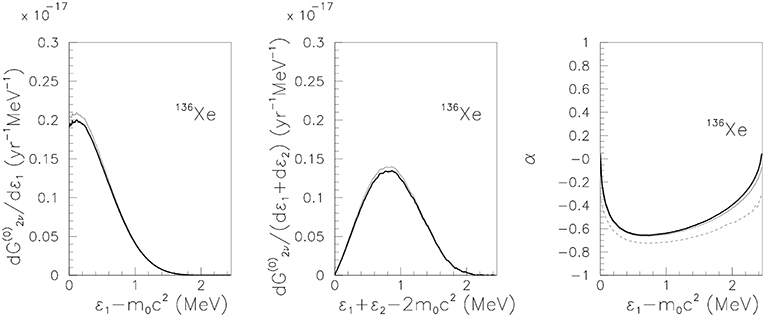
Figure 5. Same as Figure 4 for the 136Xe parent nucleus.
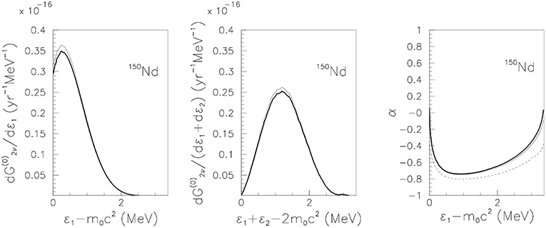
Figure 6. Same as Figure 4 for the 150Nd parent nucleus.
7. Conclusions
A review of calculated PSF involved in the β−β−, β+β+, ECβ+ and 2νECEC DBD modes is presented. Different models, from non-relativistic approaches with approximate wave functions calculations to relativistic approaches with exact electron wave functions obtained by solving numerically the Dirac equation, and with inclusion of finite nuclear size and electron screening effects are presented. For each decay mode, we present tables of PSF values for the majority of the isotopes decaying double-beta. We also compare our results with other similar ones from literature and the differences are analyzed and discussed. Finally, using our method, we also calculate the energy and angular distributions for three isotopes, namely 136Xe, 82Se and 150Nd. Accurate values of the PSF are required in the DBD investigations, in order to improve the lifetimes predictions, or the constraint the neutrino parameters [49], or for experimentalists [50], to plan their set-ups.
Author Contributions
SS and MM elaborated a new code to calculate the values of phase spaces factors involved in double-beta decay, starting with the resolution of the Dirac equation. The values reported as Stoica and Mirea [13] and Mirea et al. [39] are calculated by the authors.
Funding
The authors would like to acknowledge the support of a grant of the Romanian Ministry of Research and Innovation, CNCS-UEFISCDI, project number PN-III-P4-ID-PCE-2016-0078.
Conflict of Interest Statement
The authors declare that the research was conducted in the absence of any commercial or financial relationships that could be construed as a potential conflict of interest.
References
3. Doi M, Kotani T, Takasugi E. Double beta Decay and Majorana neutrino. Prog Theor Phys Suppl. (1985) 83:1–175.
5. Suhonen J, Civitarese O. Weak-interaction and nuclear-structure aspects of double beta decay. Phys Rep. (1998) 300:123–214.
6. Avignone FT, Elliott SR, Engel J. Double beta decay, Majorana neutrinos, and neutrino mass. Rev Modern Phys. (2008) 80:481–516. doi: 10.1103/RevModPhys.80.481
7. Ejiri H. Double beta decays and neutrino nuclear responses. Prog Part Nuclear Phys. (2010) 64:249–57. doi: 10.1016/j.ppnp.2009.12.021
8. Rodejohann W. Neutrino-less double beta decays and particle physics. Int J Modern Phys. (2011) 20:1833–930. doi: 10.1142/S0218301311020186
9. Vogel P. Nuclear structure and double beta decay. J Phys G. (2012) 39:124002. doi: 10.1088/0954-3899/39/12/124002
10. Vergados J, Ejiri H, Simkovic F. Theory of neutrinoless double-beta decay. Rep Prog Phys. (2012) 75:106301. doi: 10.1088/0034-4885/75/10/106301
12. Kotila J, Iachello F. Phase space factors for β+β+ decay and competing modes of double-β decay. Phys Rev. (2013) 87:024313. doi: 10.1103/PhysRevC.87.024313
13. Stoica S, Mirea M. New calculations for phase space factors involved in double-β decay. Phys Rev. (2013) 88:037303. doi: 10.1103/PhysRevC.88.037303
14. V A Rodin AF, Simkovic F, Vogel P. Uncertainty in the 0νββ decay nuclear matrix elements. Phys Rev. (2003) 68:044302. doi: 10.1103/PhysRevC.68.044302
15. Simkovic F, Faessler A, Rodin VA, Vogel P, Engel J. Anatomy of the 0νββ nuclear matrix elements. Phys Rev. (2008) 77:045503. doi: 10.1103/PhysRevC.77.045503
16. Simkovic F, Faessler A, Muther H, Rodin VA, Stauf M. 0νββ-decay nuclear matrix elements with self-consistent short-range correlations. Phys Rev. (2009) 79:055501. doi: 10.1103/PhysRevC.79.055501
17. Fang DL, Faessler A, Rodin V, Simkovic F. Neutrinoless double-β decay of deformed nuclei within quasiparticle randem-phase approximation with a realistic interaction. Phys Rev. (2011) 83:034320. doi: 10.1103/PhysRevC.83.034320
18. Kortelainen M, Civitarese O, Suhonen J, Toivanen J. Short-range correlations and neutrinoless double beta decay. Phys Lett. (2007) 647:128–32. doi: 10.1016/j.physletb.2007.01.054
19. Kortelainen M, Suhonen J. Improved short-range correlations and 0νββ nuclear matrix elements of 76Ge and 82Se. Phys Rev. (2007) 75:051303(R). doi: 10.1103/PhysRevC.75.051303
20. Stoica S, Klapdor-Kleingrothaus HV. Critical view on double-beta decay matrix elements with Quasi Random Phase Approximation-based methods. Nucl Phys A (2001) 694:269–94. doi: 10.1016/S0375-9474(01)00988-5
21. Caurier E, Zuker AP, Poves A, Martinez-Pinedo G. Full pf shell model study of A=48 nuclei. Phys Rev. (1994) 50:225–36.
22. Retamosa J, Caurier E, Nowacki F. Neutrinoless double beta decay of 48Ca. Phys Rev. (1995) 51:371–8.
23. Caurier E, Menendez J, Nowacki F, Poves A. Influence of pairing on the nuclear matrix elements of the neutrinoless ββ decays. Phys Rev Lett. (2008) 100:052503. doi: 10.1103/PhysRevLett.100.052503
24. Menendeza J, Poves A, Caurier E, Nowacki F. Disassembling the nuclear matrix elements of the neutrinoless ββ decay. Nuclear Phys. (2009) 818:139–51. doi: 10.1016/j.nuclphysa.2008.12.005
25. Horoi M, Stoica S, Brown BA. Shell-model calculations of two-neutrino double-β decay rates of 48Ca with the GXPF1A interaction. Phys Rev. (2007) 75:034303. doi: 10.1103/PhysRevC.75.034303
26. Horoi M, Stoica S. Shell-model analysis of the neutrinoless double-β decay of 48Ca. Phys Rev. (2010) 81:024321. doi: 10.1103/PHYSREVC.81.024321
27. Barea J, Iachello F. Neutrinoless double-β decay in the microscopic interacting boson model. Phys Rev. (2009) 79:044301. doi: 10.1103/PhysRevC.79.044301
28. Barea J, Kotila K, Iachello F. Limits on neutrino masses from neutrinoless double-β decay. Phys Rev Lett. (2012) 109:042501. doi: 10.1103/PhysRevLett.109.042501
29. Rodriguez TR, Martinez-Pinedo G. Energy density functional study of nuclear matrix elements for neutrinoless ββ decay. Phys Rev Lett. (2010) 105:252503. doi: 10.1103/PhysRevLett.105.252503
30. Rath PK, Chandra R, Chaturvedi K, Raina PK, Hirsch JG. Uncertainties in nuclear transition matrix elements for neutrinoless ββ decay within the projected-Hartree-Fock-Bogoliubov model. Phys Rev. (2010) 82:064310. doi: 10.1103/PhysRevC.82.064310
31. Neacsu A, Stoica S. Shell model calculations for neutrinoless double beta decay through the exchange of heavy neutrinos. Roman Rep Phys. (2014) 66:376–81.
32. Wang M, Audi G, Wapstra AH, Kondev FG, MacCornick M, Xu X, et al. The AME2012 atomic mass evaluation. Chinese Phys C. (2012) 36:1603–2014. doi: 10.1088/1674-1137/36/12/003
33. Haxton WC, Stephenson GJ, Strottman D. Lepton-number conservation and the double-β decay of 130Te. Phys Rev. (1982) 25:2360–9.
34. Behrens H, Janecke J. Numerical Tables for Beta Decay and Electron Capture. Berlin: Springer (1969).
38. Salvat F, Fernandez-Varea JM, Williamson W. Accurate numerical solution of the radial Schrodinger and Dirac wave equations. Comp Phys Commun. (1995) 90:151–68.
39. Mirea M, Pahomi T, Stoica S. Values of the phase space factors involved in double beta decay. Roman Rep Phys. (2015) 67:872–89. doi: 10.1063/1.4934913
40. Doi M, Kotani T, Nishiura H, Takasugi E. The energy spectrum and the angular correlation in the ββ decay. Prog Theor Phys. (1983) 70:1353–74.
41. Salvat F, Jablonski A, Powell CJ. ELSEPA-Dirac partial-wave calculation of elastic scattering of electrons and positrons by atoms, positive ions and molecules. Comp Phys Commun. (2005) 165:157–90. doi: 10.1016/j.cpc.2004.09.006
42. Salvat F, Mayol R. Accurate numerical solution of the Schrodinger and Dirac wave equations for central fields. Comp Phys Commun. (1991) 62:65–79. doi: 10.1016/0010-4655(91)90122-2
43. Esposito S. Majorana solution of the Thomas-Fermi equation. Am J Phys. (2002) 70:852–6. doi: 10.1119/1.1484144
44. Doi M, Kotani T, Nisiura H, Okuda K, Takasuki E. Neutrino mass, the right-handed interaction and the double beta decay. I: formalism. Prog Theor Phys. (1981) 66:1739–64.
45. Buhring W. Computational improvements in phase shift calculations of elastic electron scattering. Zeitschrift fur Physik (1965) 187:180–96.
46. Neacsu A, Horoi M. An effective method to accurately calculate the phase space factors for β−β− decay. Adv High Energy Phys. (2016) 2016:7486712. doi: 10.1155/2016/7486712
47. Stefanik D, Dvornicky R, Simkovic F, Vogel P. The light neutrino exchange mechanism of the 0νββ-decay with left-and right-handed leptonic and currents revisited. Phys Rev. (2015) 92:055502. doi: 10.1103/PhysRevC.92.055502
48. Simkovic F, Dvornicky R, Stefanik D, Faessler A. Improved description of the 2νββ-decay and a possibility to determine the effective axia-vector coupling constant. Phys Rev. (2018) 97:034315. doi: 10.1103/PhysRevC.97.034315
49. Barabash AS. Average and recommended half-life values for two-neutrino beta decay. Nucl Phys. (2015) 935:52–64. doi: 10.1016/j.nuclphysa.2015.01.001
Keywords: double-beta decay, phase space factors, nuclear matrix elements, neutrinos, Dirac equation
Citation: Stoica S and Mirea M (2019) Phase Space Factors for Double-Beta Decays. Front. Phys. 7:12. doi: 10.3389/fphy.2019.00012
Received: 12 November 2018; Accepted: 21 January 2019;
Published: 15 February 2019.
Edited by:
Filipe Rafael Joaquim, Universidade de Lisboa, PortugalReviewed by:
Hiroyasu Ejiri, Osaka University, JapanMario Andrés Acero O, University of Atlántico, Colombia
Copyright © 2019 Stoica and Mirea. This is an open-access article distributed under the terms of the Creative Commons Attribution License (CC BY). The use, distribution or reproduction in other forums is permitted, provided the original author(s) and the copyright owner(s) are credited and that the original publication in this journal is cited, in accordance with accepted academic practice. No use, distribution or reproduction is permitted which does not comply with these terms.
*Correspondence: Sabin Stoica, sabin.stoica@cifra.infim.ro