Influence and characteristics of anticyclonic eddies in active MHW years in the Northwest Atlantic

1 Introduction

The Northwest (NW) Atlantic is a region of economic and ecological importance (Mills et al., 2013; Pershing et al., 2018) and is among one of the fastest warming regions in the global ocean (Gonçalves Neto et al., 2021). This region also experiences extreme temperature events known as Marine Heatwaves (MHWs), defined by Hobday et al. (2016) as Sea Surface Temperatures (SSTs) exceeding the 90th percentile of the climatological mean SSTs for a minimum of 5 continuous days. These events have occurred globally under a variety of dynamics and have been increasing in intensity, duration, and frequency (Holbrook et al., 2019). Notable global MHWs include the west coast of Australia in 2010-2011 (Pearce and Feng, 2013), the Gulf of Maine in 2012 (Chen et al., 2014), the Tasman Sea in 2015-2016 (Oliver et al., 2018), the northeast Pacific in 2015-2016 (Amaya et al., 2021), and the northwest Pacific in 2021 (Kuroda and Setou, 2021). The extreme heat of MHWs causes damage to vital ecosystems through mass die-off events and altered migration patterns (Smale et al., 2019). Within the NW Atlantic, key fisheries have been affected by MHWs (Pershing et al., 2018).

The NW Atlantic has experienced four years (2012, 2016, 2017, 2020) with extreme MHWs and are considered MHW active years (Sims et al., 2022). These four years have a variety of drivers such as Jet Stream (JS) position, air-sea coupling, North Atlantic Oscillation (NAO), ocean advection from the Gulf Stream (GS) and its eddies, and latent heat flux changes (Holbrook et al., 2019; Schlegel et al., 2021). The JS has strong influence over the NW Atlantic, affecting the heat flux (Archer and Caldeira, 2008; Chen et al., 2014). The 2012 MHW formation was diagnosed as persistent JS northward shifts through the winter prior to the MHW onset (Chen et al., 2014). MHWs throughout winter and spring of 2016 were also formed and intensified under a northward shifted JS (Perez et al., 2021).

The GS is a western boundary current in the NW Atlantic, and its variability is responsible for the rapid warming in this region (Gonçalves Neto et al., 2021). The GS brings uncharacteristically warm and salty waters on the Atlantic shelf, which increases the probability of MHW formation and causes higher MHW intensities. In addition to variability, the GS meanders and sheds anticyclonic (clockwise, AE) and cyclonic (counterclockwise, CE) eddies. AEs are also known as Warm Core Rings (WCRs) due to their average warm and salty physical characteristics. WCRs tend to travel north of the GS and towards the coastline in the NW Atlantic (Saunders, 1971; Kang and Curchitser, 2013). CEs oppose AEs by being cooler, fresher eddies and are known as Cold Core Rings (CCRs; Fuglister, 1972). CEs are often found south of the GS but do not have an overall travel direction (Fuglister, 1972; Kang and Curchitser, 2013). Since 2000, AE output has doubled (Gangopadhyay et al., 2019), and shelfbreak exchanges, where warm salty waters brought onto the NW Atlantic shelf, have also increased (Silver et al., 2023). Several 2016 MHW events and the 2017 MHW event occurring in the Mid Atlantic Bight have been the result of WCR shelfbreak exchange (Gawarkiewicz et al., 2019; Perez et al., 2021).

The main objective of this work is to better understand the dynamical relationship and development of MHWs and NW Atlantic eddies. Comparing properties of eddies and MHWs in addition to oceanic parameters such as Ocean Heat Content (OHC), Mixed Layer Depth (MLD), and GS velocity will provide a better understanding of what dynamics were aiding MHW intensification and the response of these events. The depth structures of MHWs have only been recently studied in the NW Atlantic (Gawarkiewicz et al., 2019; Perez et al., 2021; Großelindemann et al., 2022; Amaya et al., 2023). In this work, GLORYS12V1 is used to observe the depth structures and development of MHWs detected at the surface through salinity and temperature in these four active MHW years. As anthropogenic warming continues, the probability of MHWs is increasing (Oliver et al., 2021). In addition, Wu et al. (2012) detects poleward shifts in western boundary currents, and poleward shifts in proxies for jet positions, which creates MHW favorable conditions along with availability of warmer temperatures. With an increase in the number of MHW events and extreme temperatures, there is more potential damage in key ecosystems (Oliver et al., 2019). In addition to ecosystem damage, long duration MHWs provide warm waters that aid in the intensification of tropical cyclones (Dzwonkowski et al., 2020; Rathore et al., 2022). Understanding MHW events and their intensification dynamics provides valuable information needed for monitoring and predicting future extreme events. With accurate predictions and monitoring, preparation for economic and environmental damage can be taken to avoid further devastation. An overview of this work’s study region and parameters used in this work and the description of the methodology of our analysis follows in section 2. Results are presented in section 3 and concluded by discussion of results in section 4.

2 Data and methods

2.1 Study area

In this study, the continental shelf-slope region of the NW Atlantic between 36°N and 46°N was examined for MHW occurrences and eddy activity. The shelf break is located at the 200-meter isobath (Figure 1), and the slope region is defined as the area between the shelf and the average path of the Gulf Stream. The average path of the Gulf Stream was identified using the 25-centimeter sea surface height (SSH) contour of monthly SSH maps spanning 2000-2020 (19 years). This method of identifying the average path of the Gulf Stream with satellite altimetry is used in multiple previous works (Lillibridge and Mariano, 2013; Rossby et al., 2014; Andres, 2016). Two geographic subregions in the NW Atlantic defined by Richaud et al. (2016), the Gulf of Maine and the Middle Atlantic Bight, were used as literature describes significant MHW events occurring there (Mills et al., 2013; Chen et al., 2014; Pershing et al., 2018; Gawarkiewicz et al., 2019; Perez et al., 2021; Schlegel et al., 2021; Großelindemann et al., 2022).

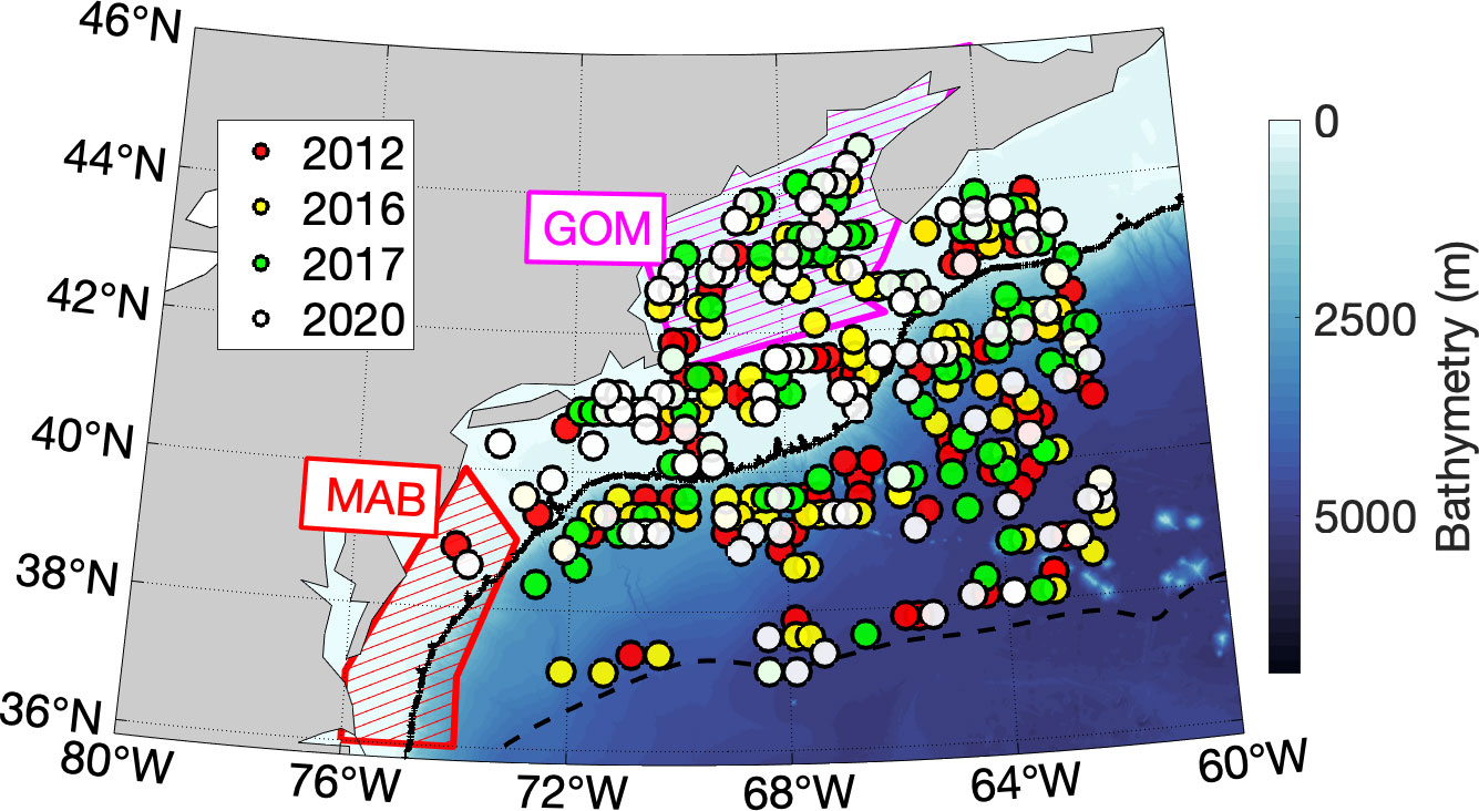
Figure 1 Map of the bathymetry of the Northwest Atlantic. Absorption positions, or dissipation, of WCRs for the four years considered here are indicated with colored dots. The dashed (black) line indicates the average path of the Gulf Stream (1993 – 2017). The solid (black) line indicates the shelf break (the 200 m isobath). Hatched boxes are sub-regions used for MHW analysis: the south shelf region, which encompasses the Mid-Atlantic Bight (MAB; red), and the center shelf region, which encompasses the Gulf of Maine (GOM; magenta).

2.2 Data

2.2.1 Satellite observations

Sea surface temperature (SST) observations were obtained from the National Oceanic and Atmospheric Administration’s (NOAA) Optimally Interpolated SST version 2.1 (OISSTv2.1), which is processed from daily blended Advanced Very High-Resolution Radiometer observations (AVHRR; Reynolds et al., 2007). OISST data has a spatial distribution of a 0.25° horizontal grid from 1981 to present at daily temporal resolution. OISST blends observations from satellites, ships, and Argo floats, allowing for high spatial and temporal resolution (Reynolds et al., 2007), and has been used to identify and characterize MHWs (Hobday et al., 2016; Schlegel et al., 2017; Oliver et al., 2018; Holbrook et al., 2019; Smale et al., 2019; Fumo et al., 2020; Perez et al., 2021; Schlegel et al., 2021).

Sea Surface Salinity (SSS) observations are provided by the European Space Agency’s Soil Moisture and Ocean Salinity (SMOS). We used debiased SMOS SSS Level 3 version 7 maps generated by LOCEAN/ACRI–ST Ocean Salinity Center of Expertise for CATDS from January 2010 to November 2021 to calculate the SSS anomalies (SSSAs) for this study. The debiased SSS are temporally averaged using a slipping Gaussian kernel with a full width at half maximum of 9 days for the 9–day product. The V7 maps are provided every 4 days, with a spatial resolution of 25 km with an applied mean over neighbor pixels at less than 30 km for the purpose of producing debiased SSS maps.

Altimetric sea level anomalies (SLAs), derived from merged multi-mission satellite observations, are currently distributed and maintained by the Copernicus Marine and Environment Monitoring Service (CMEMS; http://marine.copernicus.eu/) with a global resolution of 0.25°. SLA are referenced to a 20-year mean (1993-2012). This dataset has been previously used to track eddies associated with MHWs (Miyama et al., 2021; Yao and Wang, 2021).

2.2.2 Model simulations

GLORYS12V1 is a global implementation of the Nucleus for European Modelling of the Ocean (NEMO) platform, an eddy-resolving physical ocean reanalysis at 1/12° covering the 1993-present altimetry period. This product is distributed and maintained by CMEMS. This global ocean reanalysis, based on the real-time global high-resolution forecasting CMEMS system PSY4v3 (Lellouche et al., 2018), provides 1/12° horizontal resolution and 50 vertical levels while utilizing satellite SST measurements from NOAA and along-track satellite altimetry data from CMEMS (Pujol et al., 2016). Estimates of the three-dimensional ocean state, including sub-surface temperature, salinity, geostrophic velocity, sea surface height, and mixed layer depth were obtained from the GLORYS12v1 product. This model has been used to study surface and sub-surface characteristics of MHWs in other regions such as the Mozambique Channel (Ramanantsoa et al., 2018; Tedesco et al., 2019; Mawren et al., 2021), as well as in the Northwest Atlantic (Schlegel et al., 2021).

2.2.3 Bathymetry data

Bathymetry data was extracted from the General Bathymetric Chart of the Ocean (GEBCO), a digital bathymetry with 30 arc-second resolutions interpolated from ship depth soundings (The GEBCO_08 Grid, available at http://www.gebco.net). 95% of GEBCO bathymetry data from archival soundings is accurate to within 1.6% of depth (Marks and Smith, 2008).

2.3 Methods

2.3.1 Ocean heat content

Ocean heat content (OHC) was calculated at every grid point by integrating GLORYS12V1 temperature for the upper 300m or the upper 29 layers of the model:

where ρ₀ is the density of seawater (1025 kg m^-3), and c_p is the specific heat of seawater (3994 J kg^-1°C^-1) (Borchert et al., 2018). OHC anomaly (OHCA) was calculated using the daily climatological mean from the calculated OHC.

2.3.2 Eddy identification and tracking algorithm

Individual eddies were identified in SLA maps using the automated algorithm created by Chaigneau et al. (2008); Chaigneau et al. (2009) and Trott et al. (2018). The algorithm identifies in each daily gridded SLA field eddies defined by a center and an edge, where the center is a local extreme and the edge is the largest closed contour around that extreme. Anticyclonic (cyclonic) eddy centers are identified using local maximum (minimum) SLAs. This method detects fewer false eddies than alternative methods (Chaigneau et al., 2008; Yi et al., 2014). For each eddy, mean properties, including SSTA, SSSA, and mixed layer depth anomaly (MLDA), were computed by first averaging each parameter within each eddy, then subtracting the corresponding properties averaged between one radius and three radii from the eddy center, with warm-core (cold-core) eddies being associated with positive (negative) SSTA.

Eddy trajectories were constructed from the identified eddies using the eddy tracking algorithm defined by Pegliasco et al. (2015). This algorithm uses a cost function analysis of changes in radius, amplitude, and eddy kinetic energy (EKE) between the eddy at the first time step and any eddy at the subsequent time step that intersects the first eddy at two discrete points. If there are more than two intersections, the algorithm considers them to be the same eddy when the cost function is at its minimum. If no intersection is found between the first eddy and any eddy at the second time point, the eddy is considered dissipated, and the trajectory ends. The grid point at which the eddy dissipates is considered its absorption position. This eddy tracking algorithm is threshold-free, in contrast to other algorithms that use arbitrarily thresholded criteria (e.g., Chaigneau et al., 2008; Chelton et al., 2011).

2.3.3 MHW identification

To be classified as a marine heat wave, SSTs must exceed a seasonally varying threshold, defined as the 90th percentile of temperature variations based on a 30-year daily climatological period and must last for five or more days (Hobday et al., 2016). A 30-year climatology period is recommended to define the climatological mean to consider ocean drivers that exhibit long time scales of variability, such as the North Atlantic Oscillation (Hobday et al., 2016). The standardized marine heat wave definition from Hobday et al. (2016) was applied to daily remotely sensed SST data spanning 1993 to 2021 to compute temperature anomalies and analyze events in 2012, 2016, 2017, and 2020 (Reynolds et al., 2007).

MHWs are characterized by various metrics. MHW intensity is defined as the positive temperature anomaly occurring during MHW events and often averaged temporally over the duration of the event or spatially through a defined region. This procedure is also applied to salinity anomalies during MHW events throughout this work. The number of MHW events per year is defined as the number of discrete events at each grid point per year, whereas the total number of MHW days is the sum of days experiencing MHWs at any grid point. The value of total grid points experiencing MHWs is also given for each year.

2.3.4 Root mean square error

To understand the effect that AEs have on MHWs, the MHW properties of SSTA intensity, SSSA intensity, OHCA, and MLD are observed as average timeseries before and after a MHW and AE interaction. Root mean square error (RMSE) is calculated between the mean timeseries and each interaction’s timeseries to account for variability between each event. RMSE was calculated by:

where X and X_mean represent the four time series and their means, while N is the number of interactions between MHWs and eddies.

2.3.5 Gulf Stream eddy heat flux convergence

To understand the influence of the GS on MHW intensity and AEs, the eddy heat flux convergence (EHFC) is calculated and averaged along the 25 cm SSH contour, which indicates the average path of the GS. Horizonal and vertical terms of EHFC were calculated using GLORYS12V1 velocity (V), temperature (T), and SSH (η) products. Horizontal EHFC is calculated by:

where V’ and T’ are known as the perturbation term and are the result of velocity and temperature subtracted by the time averaged mean (Zheng et al., 2022). Vertical EHFC is calculated by:

These equations were determined from the Reynolds average thermal energy equation used for upper-ocean heat content variability in Zheng et al. (2022).

3 Results

3.1 AE and MHW presence in the NW Atlantic

In the MHW active years (2012, 2016, 2017, and 2020), there are 475 distinct eddy absorption events within the NW Atlantic (Figure 1). The GOM had between 45-60 AE absorptions with an average of 566 detected AEs during these MHW active years. The MAB has on average 3 AE absorptions and a range of 8-22 detected eddies. The MAB had significantly less eddies than the GOM. Total number of absorption eddy events in the NW Atlantic was 128 for 2012, 114 for 2016, 103 for 2017, and 130 for 2020 (Figure 1). Perez et al. (2021) describes 2016 as a year with abnormally more WCR absorptions, yet 2012 and 2020 had more total absorptions within the NW Atlantic. 2020 had the most eddies in the NW Atlantic and both subregions, there is not a significant difference between these years. 2017 and 2016 have fewer eddies that tend to be longer lived than 2012 and 2020.

In the NW Atlantic, there were 43355 MHW events detected in the four MHW active years (Figure 2). 2017 had the least events, while the other years were closer together with 2016 having the most events. On average the GOM had 2080 MHWs and the MAB had 1140 (Figure 2). The GOM experiences more MHW events in these four years than the MAB. The 2012 MHWs overall had a high frequency near the coastline, especially in the GOM and the Scotian shelf (Figure 2A). The 2016 MHWs were widespread throughout the NW Atlantic (Figure 2B). Both 2017 and 2020 had a high frequency of events along the GS but 2020 also had events concentrated on the shelf near Cape Cod (Figures 2C, D).

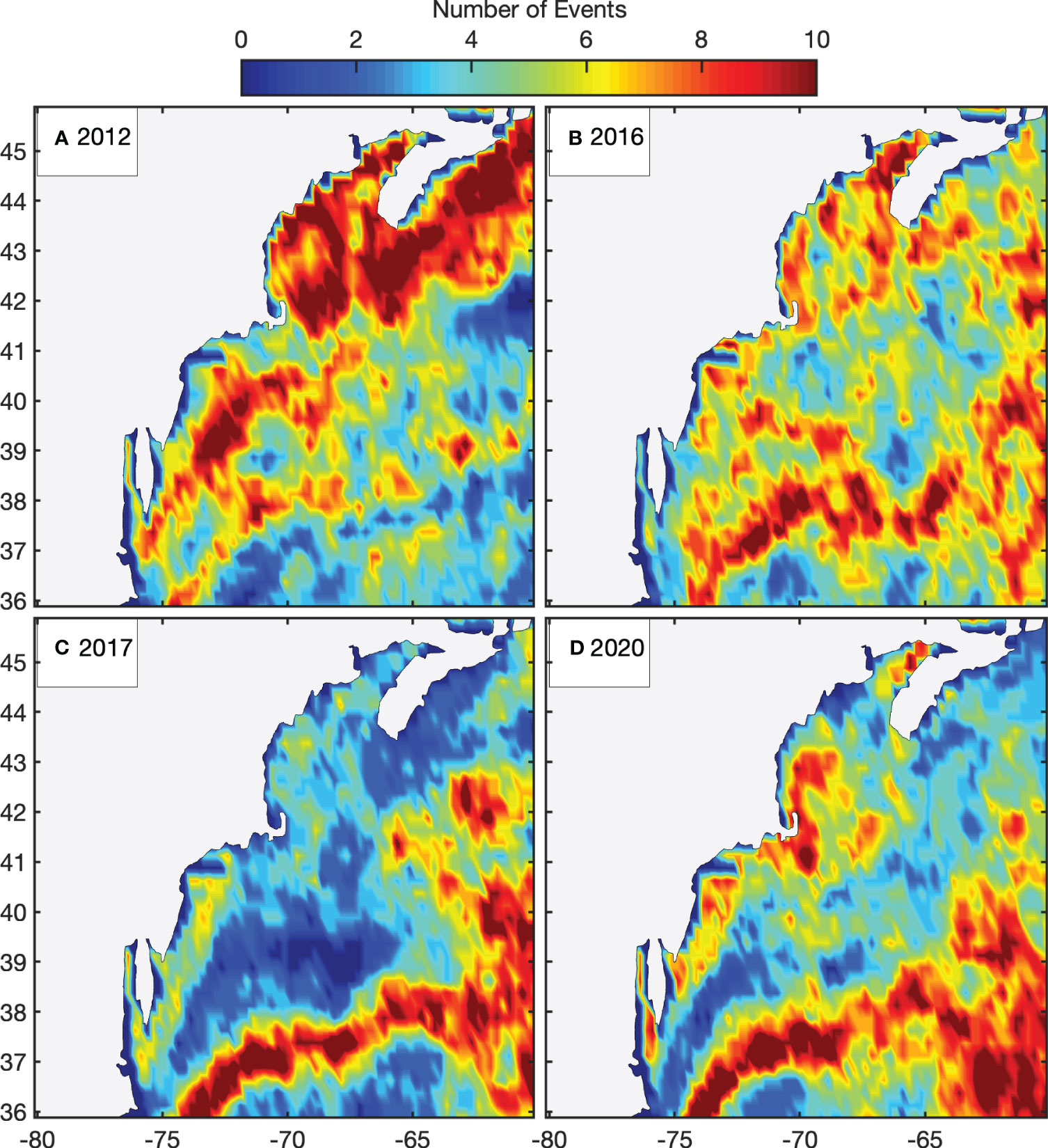
Figure 2 Map depicting the number of discrete MHW events for 2012 (A), 2016 (B), 2017 (C), and 2020 (D).

In 2012, the MAB experienced the maximum mean MHW SSTAs of 2.3°C in July, with the maximum SSTA peaking in April (Figure 3A). SSSAs at the maximum mean SSTA is low, while SSSAs during the maximum SSTA is high (Figure 3A). The 2012 GOM had low SSSA with little variability throughout the year (Figure 3B). The mean and maximum SSTAs in the GOM increased from January until May, reaching a peak at 1.7°C (Figure 3B). These GOM MHWs found in the early part of the year are atmospherically forced (Chen et al., 2014). The 2016 MAB maximum mean SSTA is 2.4°C in August, which aligns with a minimum in maximum SSTA and mean SSSA (Figure 3C). This month had low intensity events with widespread atmospherically forcings (Figure 3C; Perez et al., 2021). March through April experiences another peak SSTA with a high mean SSSA, aligning with AE driven events (Figure 3C; Perez et al., 2021). The maximum mean MHW SSTA in the GOM occurs in September (1.7°C) after increasing since May (Figure 3D). The maximum SSSA peaks are in August and February which coincide with maximum SSTA peaks (Figure 3D). The MAB and GOM both have high SSTA and SSSA in August; this is when Perez et al. (2021) observe that much of the NW Atlantic was experiencing widespread MHWs (Figures 3C, D). The 2017 MAB experiences a peak mean and maximum SSTA (0.9°C; 1.3°C) in March, which occurs simultaneously with a high mean SSSA (1 psu; Figure 3E). From January through April, a MHW driven by a WCR passed through the MAB, peaking in intensity during March (Figure 3E; Gawarkiewicz et al., 2019). The 2017 GOM has on average a high mean SSSA (Figure 3F). There is a peak in mean SSTA in June that occurs with high SSSA, but the maximum mean SSTA (2.2°C) occurs at a minimum SSSA in November 2017, following the pattern of 2012’s atmospherically driven MHW event (Figures 3B, F). The 2020 MAB peak mean SSTA (1.2°C) in February aligns with maximum SSSA peak but mean SSSA is low, indicating no widespread ocean-driven event (Figure 3G). The MAB has low SSSA and SSTA from June through September (Figure 3G). The GOM maximum mean SSTA (1.8°C) in August (Figure 3H). Low mean SSSAs are prevalent throughout the year but summer months experience high maximum SSSAs in June that align with maximum SSTA (Figure 3H).

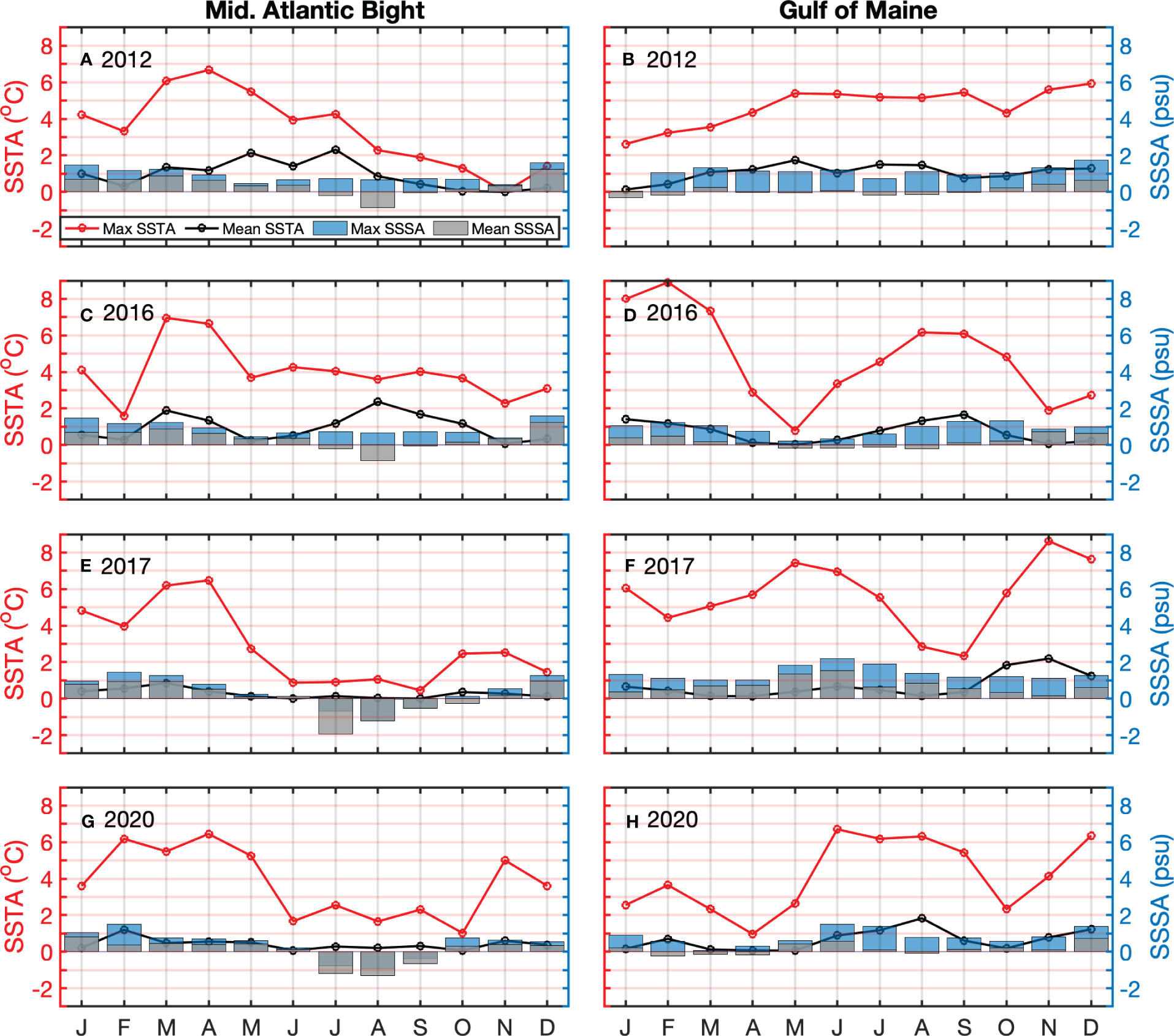
Figure 3 Time series depicting the monthly mean (black) and monthly maximum (red) intensity of MHWs in the MAB (left) and in the GOM (right). Barplots depict the monthly mean (black) and monthly maximum (blue) SSSA anomalies during MHWs of 2012 (A, B), 2016 (C, D), 2017 (E, F), and 2020 (G, H) in the two regions.

3.2 Eddy properties during MHW active years

The maximum mean SSTA intensities in the GOM occur in May 2012, September 2016, November 2017, and August 2020 (Figure 3). May 2012 had a high number of AEs around the GOM (Figure 4A). September 2016 had more AEs further off the shelf (Figure 4B). November 2017 follows a similar distribution to 2012, with more AEs also along the GS (Figure 4C). August 2020 has a similar spatial distribution of AEs to 2016 (Figure 4D). The similar distribution of AEs in 2012 and 2017 lead to peak intensities in the GOM by moving warmer waters into a region already in a MHW state, thereby extending the duration of the state. 2016 and 2020 GOM mean intensities quickly decrease after the peak (Figure 3), indicating processes encouraging MHW decay in the absence of AEs. Low AE radius and low amplitude was seen between these selected months (Figures 4E–L). Overall low SSTA and SSSA are also present in these months (Figures 4M–T). Between 40-42°N, higher AE radius and amplitude and more extreme SSTA and SSSA are observed. The higher selected AE radii exceeds 90 km and amplitude exceeds 3.3 cm, with 2020 having the highest radii and amplitude and 2017 having the lowest. The mean SSTA between 40-42°N was 0.2°C across these four months (Figures 4M–P). Below 40°N, 2012 experiences unusually strong negative AE SSTAs, indicating that these AEs have moved into an area with higher average SST than where they originated, such as the GS or Sargasso Sea, leading to the negative SSTAs (Figure 4M). Negative AE SSSA are present around the GOM in 2012, the Scotian shelf in 2016 and 2017, and above the MAB in 2020 (Figures 4Q–T).

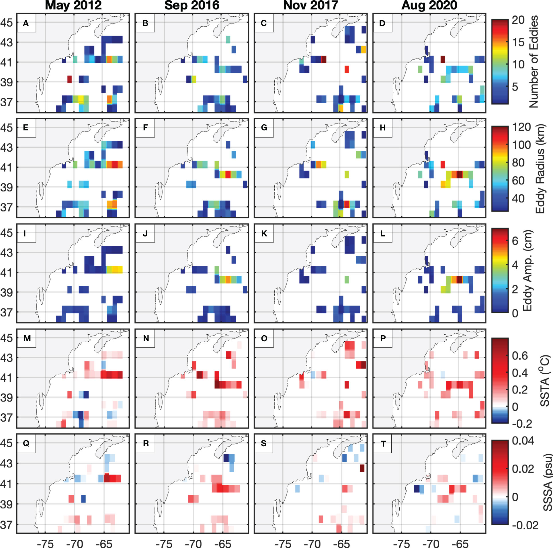
Figure 4 Mean spatial distribution of anticyclonic eddy characteristics during the months of highest MHW intensity within the GOM in 2012, 2016, 2017, and 2020 (left to right columns). Characteristics are number of eddies (A–D), radius (E–H); km, amplitude (I–L); cm), SSTA [(M–P °C], and SSSA (Q–T); psu.

From 2012 to 2021, there were 4.7-8 AEs and 6.8-10.4 CEs, with no overall trend (Figure 5A). During the 2012 MHW period (February-July) AEs decreased, while CEs are consistent (Figure 5A). 2016’s MHW period (April-September) has less variability than 2012 but follow a similar pattern (Figure 5A). In 2017’s MHW period (March-November) and 2020’s MHW period (January-September) had a consistent values of AEs and CEs (Figure 5A). The average amplitude (6.8 cm), radius (57.3 km), and EKE (204.3 cm² s^-2) of AEs and CEs in the MHW periods of 2012, 2016, and 2017 are noticeably lower and have less variability than the rest of the time series (Figures 5B–D). 2020 MHW period has a minimum of AE amplitude, radius, and EKE in late March, with maximum of AE and minimum of CE in amplitude, radius, and EKE in September (Figures 5B–D). Similar peaks are seen in September 2013, October 2014, November 2015, April 2018, and September 2021 (Figures 5B–D).

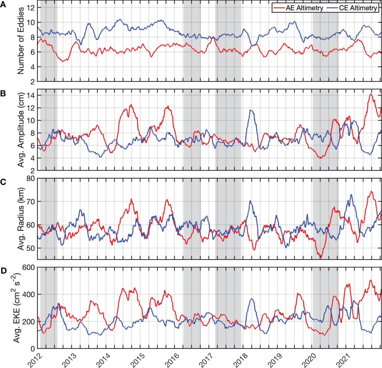
Figure 5 Time series of average anticyclonic eddy (AE) and cyclonic eddy (CE) characteristics, number (A), amplitude (B), radius (C), and EKE (D), found in the shelf-slope region between 2012 and 2020. Gray shading indicates MHW periods.

3.3 The interplay of eddies, MHWs, and GS eddy heat flux convergence

Prior to the interaction between MHWs and AEs, temperature intensity increases to an average peak of 3.3°C before declining (Figure 6A). RMSE is inverse to the mean time series, indicating that the peak temperature intensity is better at representing MHW dynamics at the interaction peak (Figure 6A). SSSA and the RSME have little variability (Figure 6B). OHCA peaks one day prior to the MHW-AE interaction, and rapidly declines one day after (Figure 6C). Between five days prior and 3 days after the interaction, the RMSE decreases and remains constant to the end of the observed time series (Figure 6C). MLD and the RMSE reach a peak 3 days after the interaction (Figure 6D). The temperature and salinity anomalies composites with depth show the average changes that occur during these events from 1993 through 2020. The temperature anomaly maximum at 13.5 m persists through the event (6.4°C; Figure 6E). High temperature anomalies (above 3.9°C) were in the upper 100 m prior to day 0 of this interaction (Figure 6E). Maximum temperature intensities of the MHW events become slightly deeper after interacting with AEs. Salinity anomalies from the surface to 40.3 m change only slightly through these events, remaining below 2.0 psu (Figure 6F). Days prior to the event had consistent salinity anomalies between 2.1-2.3 psu below 50 m (Figure 6F). The maximum salinity anomaly was 2.3 psu 5 days prior to the event. After the event, salinity anomalies tended to decrease with depth but remained above 2.1 psu (Figure 6F). Overall, AEs interacting with MHWs increase OHC leading up to the event, deepen the range the MHW impacts, and affect the surface temperature variability (Figure 6).

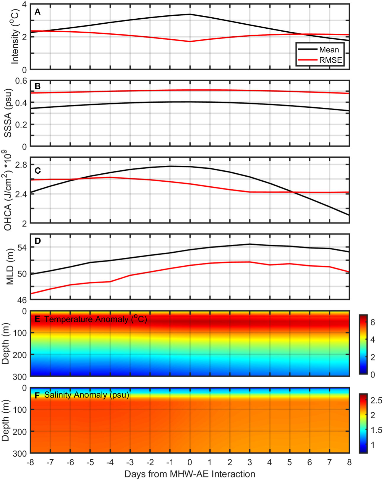
Figure 6 Average time series (black) of SSTA intensity (A), SSSA intensity (B), Ocean Heat Content anomalies (C), and Mixed Layer Depth (MLD, D) and the root mean square error (red) for MHW are shown 8 days before and after interacting with AEs. Composite temperature anomalies (°C) and salinity anomalies (psu) up to 300 m depth (E, F) of MHW events are also shown up to 8 days before and after interaction of these events.

The number of AEs for each MHW active year is relatively consistent, with a mean in the GOM at 6.7 eddies and in the MAB at 7.4 eddies (Figures 7A–D). AE numbers in the MAB and the GOM decreased throughout the active MHW years, except in the 2020 in the GOM, which did not have a decreasing trend (Figures 7A–D). While the decreasing trend in the subregions reflect the overall NW Atlantic trends for 2012, 2016, and 2017, this trend is not seen during the observed years in Figure 5. The GOM AE numbers do not relate to GOM MHW intensity (Figures 7A–D). The high MAB AE numbers, above 7.5 eddies, in spring of 2012, 2016, and 2017 have a concurrence of high MAB MHW intensity above 3.5°C (Figures 7A–C). The AE radius in the GOM for all four years averages to 62.8 km with low variability and are larger than MAB AEs (Figures 7E–H). 2020 experiences smaller AEs, an effect which is pronounced in the MAB (Figure 7H). 2016 and 2017 AE radii increased throughout their respective years (Figures 7F–G). There was no relationship between AE radius and MHW intensity (Figure 7E–H). EKE also had no relationship with MHW intensity (Figures 7I–L). EKE is more variable than other eddy characteristics. Unlike in Figure 5, simultaneous AE radius and EKE peaks are not evident in Figure 7E–L. 2012 and 2016 have higher average EKEs in the MAB than the GOM, while 2017 and 2020 show the opposite relationship (Figures 7I–L).

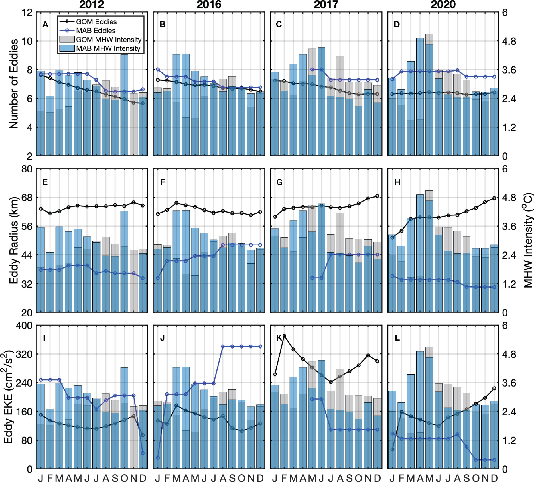
Figure 7 Time series of monthly-averaged AE characteristics located within the GOM (black) and within the MAB (blue) for the selected four years (A–L), plotted against monthly-averaged MHW intensity in the GOM (black) and in the MAB (blue).

To further understand the relationship between MHWs and their possible drivers, they are compared in a Lead-Lag Cross-Correlation in both subregions for each MHW active year (Figure 8). The MAB consistently showed low correlation values, below 0.3, in the following pairs: MAB AE EKE and MHW events, AE EKE and MHW intensity, and GS EHFC and AE EKE (Figure 8). Values below 0.44 with less than 15 lag days in 2012, 2016, and 2020 were observed in the GoM for AE EKE and MHW intensity as well as GS EHFC and AE (Figures 8A, B, D). 2017 has correlations for these same parameters above 0.65 and has the largest lag for AE EKE and MHW intensity (Figure 8C). 2012 and 2016 share a pattern of GS EHFC lagging AE EKE, while in 2017 and 2020 GS EHFC leads (Figure 8). The shift between 2016 and 2017 is likely from the increased GS variability that started in late fall 2016, but this does not explain the 2020 pattern (Andres, 2021; Perez et al., 2021). In all MHW active years, GS EHFC and MHW intensity have correlations above 0.75 with lag days between -15 and 15 for both subregions (Figure 8). 2017 has the strongest correlation of this parameter pair and 2016 has correlations between each subregion closer than any other parameter pair (Figures 8B, C). GS EHFC is a metric of near-surface transport of heat by the GS, and MHWs are intensifying from the heat brought by the GS to these subregions in these four MHW active years (Zheng et al., 2022).

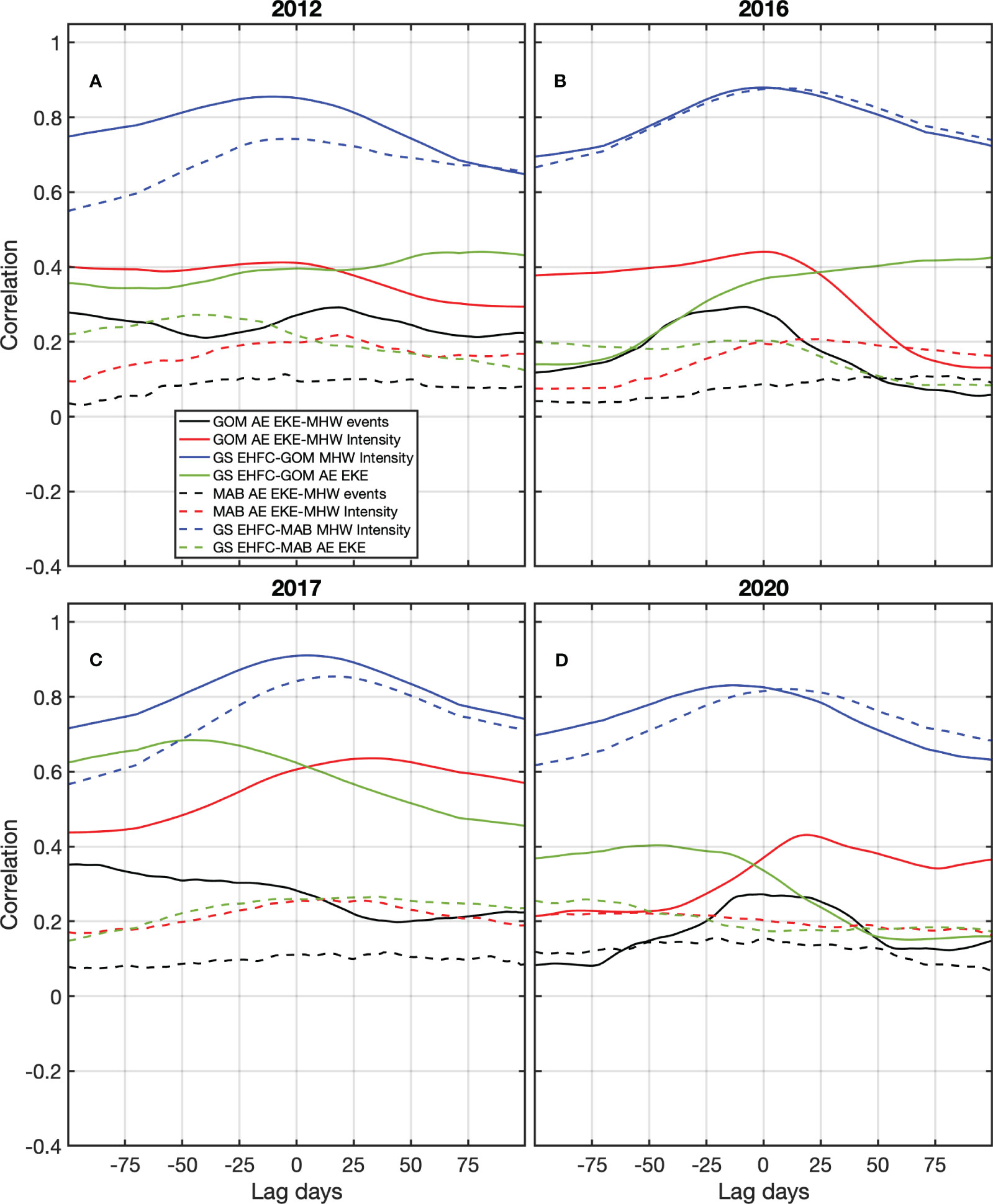
Figure 8 Lag-Lead Cross-Correlation of AE EKE and MHW events (black), AE EKE and MHW Intensity (red), GS Eddy Heat Flux Convergence (EHFC) and MHW Intensity (blue), and GS EHFC and AE EKE (green) for 2012 (A), 2016 (B), 2017 (C), and 2020 (D). AE EKE, MHW events, and MHW Intensity are compared between subregions of the GOM (solid) and the MAB (dashed).

3.4 Depth comparison of MHW active years and their MHW events

High temperature anomalies above 2.2°C exceed 100 m in May through July 2012 during the duration of the atmospherically forced MHW (Chen et al., 2014) as shown in Figure 9A. Additional high temperature anomalies are found between 55-77m in September and December; this subsurface heating may indicate peaks in subsurface MHW intensities that go undetected from surface observations (Figure 9A). During high temperature anomalies in May through July 2012 (Figure 9A), a high salinity anomaly forms below 40 m, reaching a maximum of 0.5 psu (Figure 9B). 2016 high temperature anomalies above 1.6°C are present January through March throughout the upper 100 m and in June and October at 55.8 m (Figure 9C). GOM 2016 positive salinity anomalies are observed to exceed 100 m in January through March and August through September, aligning with high subsurface temperature anomalies (Figure 9D). January through March and fall 2016 were recorded as months when subregions in the NW Atlantic experienced MHWs that coincided with an increase in AE absorption and GS variability (Perez et al., 2021). 2017 GOM temperature anomalies above 1°C are present through the upper 100 m in February, June through August, and October through December (Figure 9E). Salinity anomalies in 2017 are low, averaging 0.1 psu from January through November (Figure 9F). The GOM in 2017 contained greater than average SSSAs in MHW grid points among the other MHW active years but the GOM as a whole did not have higher than average salinities (Figure 9F). 2020 temperature anomalies in the GOM are the lowest in these four years (Figure 9G). The notable high temperature anomalies in 2020 that exceed 1.0°C were in June through August above the mixed layer or below 80m, February below 80m, and December exceeding 100m (Figure 9G). Salinity anomalies outside of December in 2020 GOM average below 0 psu (Figure 9H).

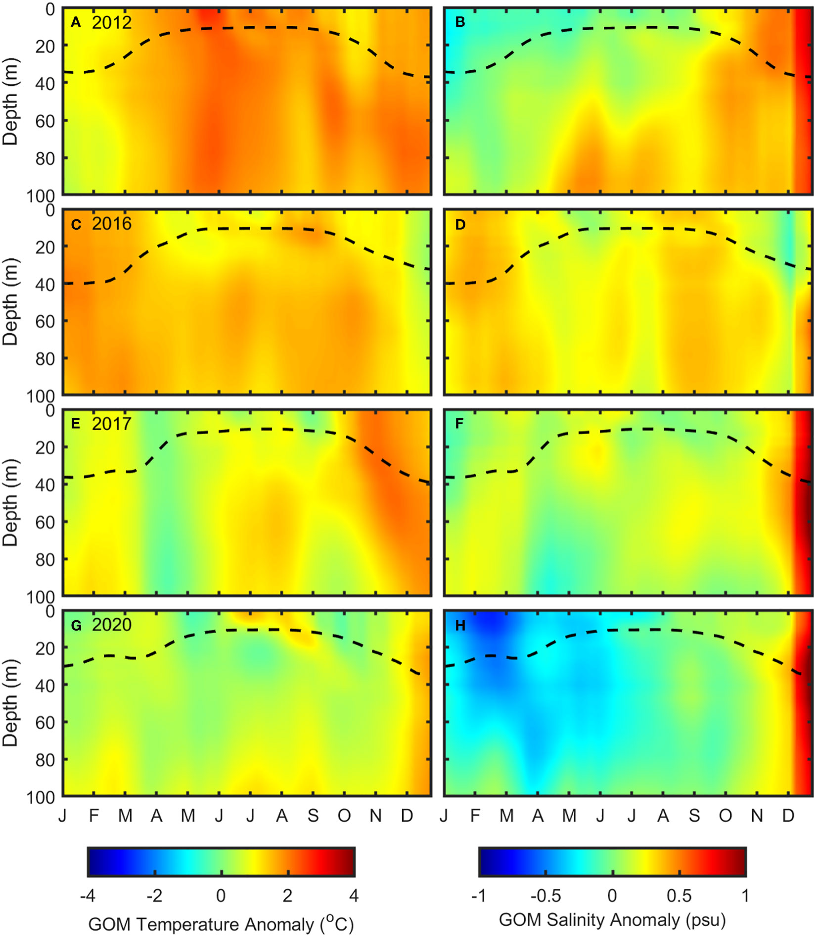
Figure 9 Monthly depth temperature anomaly left; (A, C, E, G) and salinity anomaly right; (B, D, F, H) composites of the upper 100 m of the water column over the GOM. Monthly mixed layer depths plotted with black dashed lines.

2012 MAB has high temperature anomalies above 2.2°C in January through July ranging between 80 m and 100 m (Figure 10A). Higher salinity anomalies are seen in January between the surface and 80 m, in April through May between 40 m and 100 m, in June within the MLD, and in July through mid-August below the MLD (Figure 10B). 2016 has high temperature anomalies above 1.4°C extending from the surface or the mixed layer depth through the upper 100 m for most of the year, with maximums in March through April (Figure 10C). The 2016 MAB has high salinity anomalies through most of the year coinciding with high temperature anomalies (Figure 10D). Negative surface salinity anomalies occur in July (Figure 10D). The MAB in spring 2016 experienced several WCR absorption events, leading to warmer and saltier waters (Perez et al., 2021). High temperature anomalies occur in January through April and October 2017, while June through September has negative temperature anomalies (Figure 10E). Salinity anomalies exceed 0.3 psu at the surface in January through April and in December (Figure 10F). These results are contextualized by Gawarkiewicz et al. (2019), who recorded the MAB MHW from January to April following a WCR intrusion of the MAB shelf with a distinct salinity anomaly remaining after the MHW’s decline. In 2020, high temperature anomalies above 1.0°C extended from the surface to 100 m in February and March, from the surface to 51 m in November through December, and below 40.3 m in June (Figure 10G). A subsurface low anomaly (-1.4°C) is present from 30-100 m in July through September (Figure 10G). The only overlap of high salinity and temperature anomalies is in November through December above the MLD (Figure 10H). Negative salinity anomalies occur at the surface in March, May, and July and below 50 m from July into October (Figure 10H). The 2020 MAB has the lowest temperature and salinity anomalies in these MHW active years (Figures 9, 10).

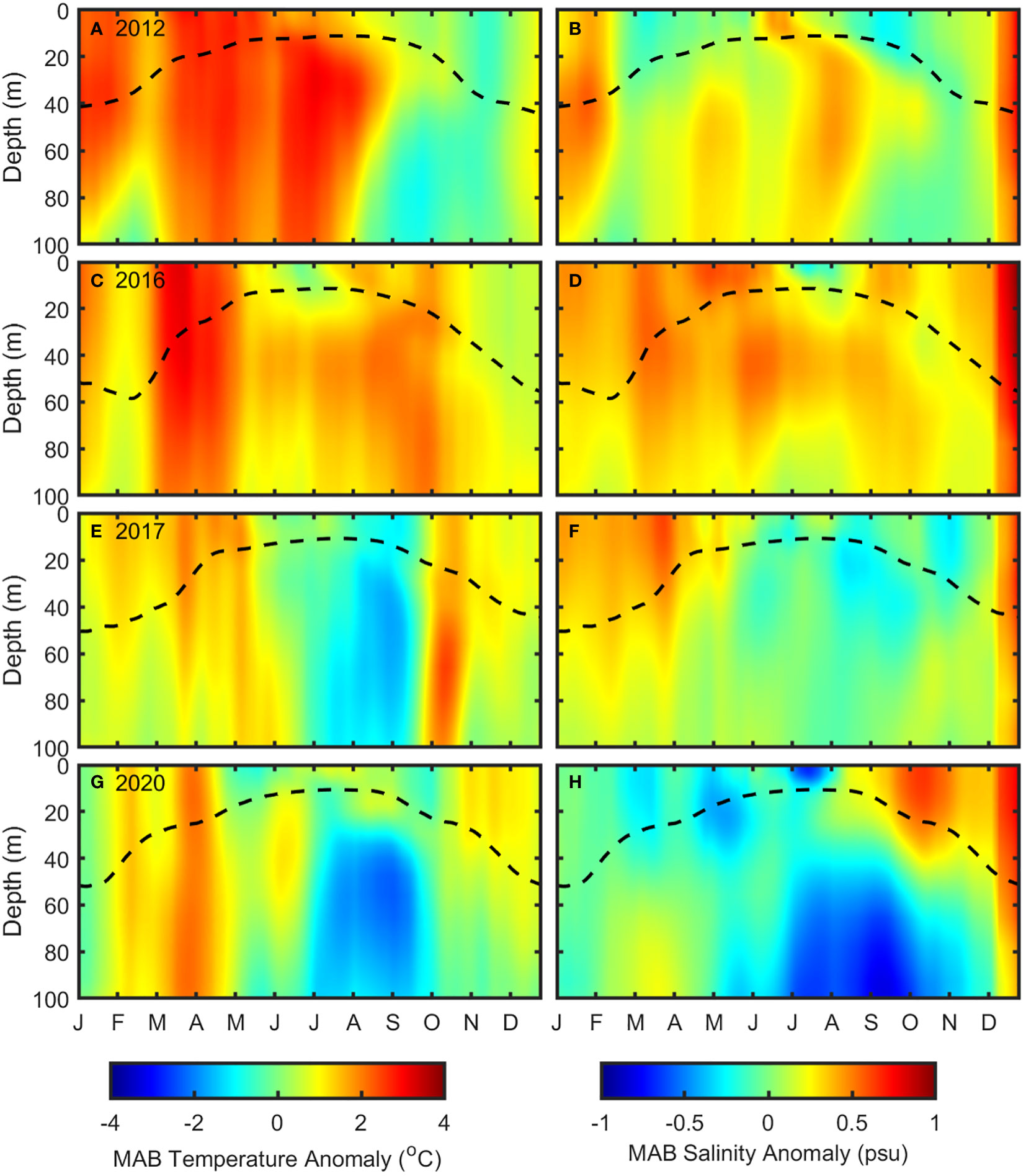
Figure 10 Monthly depth temperature anomaly [left; (A, C, E, G)] and salinity anomaly [right; (B, D, F, H)] composites of the upper 100 m of the water column over the MAB. Monthly mixed layer depths plotted with black dashed lines.

The 2012 GOM MHWs remain above 2.0°C in the upper 60 m but quickly decrease and reach a minimum of 1°C at 186.1 m (Figure 11A). The 2012 GOM MHW salinity anomalies remain around 0.4 psu from the surface until 130.7 m (Figure 11B). The most extreme 2012 GOM MHW events occurred below the surface and the lack of abrupt changes in the oceanic profiles reflect the dynamics of widespread atmospheric forcings that are present in 2012 (Figures 11A, B) as also observed by Chen et al. (2014). The 2016 GOM MHWs remained near 2.0°C above 70 m before decreasing (Figure 11A). 2016 has strong surface GOM MHW salinity anomalies that decrease to 0.3 psu at 155.9 m (Figure 11B). 2017 has the highest GOM MHW temperature anomalies in the surface mixed layer and overall, reaching 3.5°C at 34.4 m (Figure 11A). 2017 MHW salinity anomalies decrease from 1.0 psu at the surface to 0.3 psu at 100 m (Figure 11B). The peak of the average MHW temperature anomaly aligns with the peak temperatures in October through December in Figure 9E, further indicating these months as the most extreme MHW events in 2017 GOM. These 2017 MHWs also experience more abrupt changes in temperature and salinity at shallow depths than other profiles (Figures 11A, B). 2020 MHW temperature anomalies have a subsurface peak of 2.4°C at 109.7 m (Figure 11A). 2020 salinity anomalies also have a subsurface maximum of 0.5 psu at 130.7 m, slightly below the temperature anomaly (Figure 11A, B). The lower temperature and salinity anomalies for 2020 MHWs in the upper 100 m are consistent with the low average temperature and salinity anomaly averages demonstrated in Figure 9G and 13H. The peak 2020 MHW temperature and salinity intensity occurs below 100 m, the depth considered to have the most intense MHWs (Großelindemann et al., 2022).

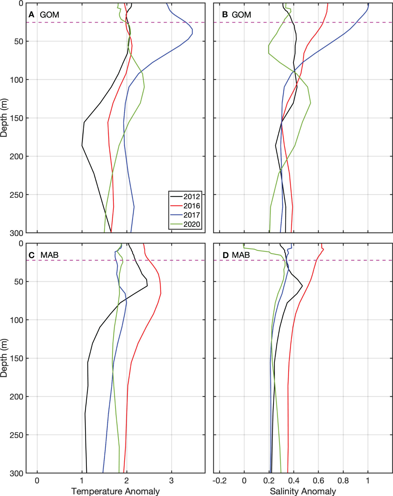
Figure 11 Temperature (A, C) and salinity (B, D) profiles of averaged MHW properties in each subregion up to 300 m during the four years in GOM (A, B) and MAB (C, D). Average mixed layer depth for subregion between 2012 and 2020 is represented by the dashed magenta line (GOM MLD: 25.494 m; MAB MLD: 22.4 m).

The 2012 MAB MHW temperature anomalies increase from 2.0°C to 2.5°C, peaking at 55 m before steeply dropping (Figure 11C). 2012 MHW salinity anomalies reach a maximum at 0.5 psu at the same time as the peak in temperature anomalies (Figure 11D). The MHW temperature and salinity anomaly maxima reflect the depth where the major anomalies are in Figures 10A, B (Figures 11C, D). As previously noted, the 2012 MHWs were largely atmospherically forced (Chen et al., 2014), but AEs were also intensifying events in the MAB, specifically during January, May, and July (Figure 10B). The 2016 MAB MHW temperature anomalies have a maximum of 2.8°C at 66 m and stay above 2.0°C until 250 m (Figure 11C). MHW salinity anomalies decreased from 0.6 psu to below 0.4 psu throughout the water column (Figure 11D). 2016 MHW temperature and salinity profiles mirror the change in slope in each subregion, indicating the drivers of 2016 MHWs influencing both temperature and salinity but with different strengths across the subregions (Perez et al., 2021). For MAB MHWs, 2016 has the most intense MHWs across these four MHW active years (Figures 11C, D). The 2017 MHW temperature anomalies remain around 1.7°C but reach a subsurface maximum of 2.0°C at 78 m (Figure 11C). The salinity anomalies have very little variability but decrease from 0.4 psu at the surface to 0.2 psu below the surface layer (Figure 11D). Fewer 2017 MHW events occurred throughout the year, which those that did form tending to have low surface temperature and salinity intensity (Figures 2, 3). The MAB also experienced low temperature and salinity anomalies throughout the summer and early fall (Figures 10E, F), leading to MHWs not having a strong influence upon the vertical profiles. Surface MHWs anomalies are influenced by WCRs in January through April, which caused warm waters to cross the 100 m isobath. However, due to additional MHWs of lower temperature intensity, the average profile has little overall intensity (Gawarkiewicz et al., 2019). 2020 MHW events in the MAB had relatively uniform temperature anomalies with depth and salinity anomalies were similarly constant below the mixed layer (Figures 11C, D).

4 Discussion

The NW Atlantic experienced four MHW active years in 2012, 2016, 2017, and 2020. Each year had unique formations and developments of their MHW events. 2020 and 2012 experienced more AE absorptions that 2016 and 2017, despite Perez et al. (2021) showing that 2016 had an anomalously high absorption (Figure 1). 2016 and 2017 AEs had longer durations, likely due to increased GS variability occurring in these years (Andres, 2021; Perez et al., 2021). 2012 likely experienced AE related intensification along with 2020, even as 2012 is known as an atmospherically driven year (Chen et al., 2014). 2016 had the most MHWs spread across the NW Atlantic, while 2012 had the most MHWs along the Atlantic shelf (Figures 2A, B). 2017 and 2020 had MHW events contained along the GS, with some events in 2020 along the coastline (Figures 2C, D). MHWs in the GOM and the MAB also had different formations between the subregions and also throughout the duration of the year (Figure 3). The MAB experienced higher average MHW SSSA intensity than the GOM but both regions experienced low SSSA during the months with highest MHW SSTAs (Figure 3). Low and negative average SSSAs occurred throughout the year, except for 2017 and during peak MHW intensity in the GOM (Figures 3B, D, F, H).

The spatial properties of AEs during the most active GOM MHW months reveal a pattern of higher extreme AE properties between 40-42°N, likely due to AE shedding (Figure 4; Kang and Curchister, 2013). In this region, SSTA and SSSA of AEs were more extreme than surrounding AEs, radii exceeded 90 km, and amplitude exceeded 3.3 cm (Figure 4). 2017 and 2016 were the least extreme two years, in addition to lower numbers of AE absorptions and longer durations (Figures 1,4). This further connects 2016 and 2017 MHW and AE dynamics to the increase in GS variability (Andres, 2021; Perez et al., 2021). A comparison of AE and CE properties reveals high variability from 2012 to 2021, but 2012, 2016, and 2017 all experienced low variability and values in average amplitude (6.8 cm), radius (57.3 km), and EKE (204.3 cm²s^-2) (Figures 5B, D). The NW Atlantic also experienced more daily CEs than AEs throughout the observed timeseries (Figure 5A), though they are not generally a driver of MHW intensification (Kang and Curchitser, 2013; Schlegel et al., 2021).

AEs interacted with MHW properties such as SSTA intensity, OHCA, and MLD (Figure 6). SSTA intensity and MLD increased during AE interactions, while OHCA decreased after the event (Figure 6). Depth composites show AEs tending to increase the depth of higher temperature anomalies with little effect on salinity (Figures 6E, F). AE radius and EKE did not have an obvious relationship with MHW intensity, but MAB AE number and MHW intensity reached concurrent peaks in the spring of 2012, 2016, and 2017 (Figure 7). At that time, the MAB experienced MHWs due to JS variability in 2012 and 2016, GS variability in 2016, and an AE absorption in 2017 (Chen et al., 2014; Gawarkiewicz et al., 2019; Perez et al., 2021). Lead-Lag Cross-Correlations show AE EKE and MHW events have the overall weakest correlation, indicating that AEs are not the primary driver of MHWs in both subregions (Figure 8). GS EHFC and MHW intensity had correlations above 0.75 for all years in both subregions, with 2017 having had the highest correlation in the GOM (Figure 8). 2016 had the second highest correlation of GS EHFC-MHW intensity with identical values in both subregions. Heat from the GS was being transported to these subregions and directly intensifying MHWs in these four years. 2012 and 2016 share the pattern of GS EHFC lagging AE EKE, while 2017 and 2020 share GS EHFC leading AE EKE. From late 2016 through 2017 the GS experienced higher variability (Andres, 2021; Perez et al., 2021), which may have played a role in the large shift in pattern and the two highest correlations in the GS EHFC and MHW intensity. 2012 was reported to be mainly atmospherically forced MHW events (Chen et al., 2014), but there was a clear influence of oceanic drivers. 2016 had multiple drivers that affected different subregions at select times (Perez et al., 2021) and likely 2012 and 2020 followed this pattern with stronger dependence on atmospheric forcings.

Monthly depth temperature and salinity anomalies during the MHW active years allow insight into surrounding conditions to the MHW events (Figures 9, 10). Chen et al. (2014) states the MAB and GOM experienced some of the warmest ever temperatures in early 2012; this is supported by the extreme temperature anomalies in Figures 9A and 10A. The GOM and the MAB salinity anomalies in 2012 had different responses throughout the year, as higher salinity in the GOM gradually filled the water column while the MAB higher salinity was only seen to coincide with extreme temperatures (Figures 9B, 10B). Both subregions in 2016 experienced high temperature and salinity anomalies during increases in AE absorptions and noticeable GS variability (Figures 9, 10; Perez et al., 2021). 2020 was the coolest and freshest MHW year in the GOM and MAB and 2017 had variable anomalies throughout the year, but both lacked the consistent extreme temperature and salinity anomalies of 2012 and 2016 (Figures 9, 10). The 2017 MAB did show high temperature and salinity anomalies from January through April that followed the AE intrusion studied by Gawarkiewicz et al. (2019) and high temperature anomalies in October that aligned with low MHW intensity as in Figure 3E (Figure 10E, F).

MHW depth profiles detail the average MHW structure in the subregions for each year (Figure 11). The 2012 GOM MHW events reached an average maximum intensity at 40.3 m; this shallower depth of MHW temperature and salinity for 2012 reflects the dynamics common in atmospherically forced MHWs (Figures 11A, B; Chen et al., 2014; Oliver et al., 2021). In contrast, the 2012 MAB profile peaked at 55 m and quickly decreased below (Figures 11C, D). While the JS variability forced MHW events across the NW Atlantic, there was likely an AE or GS influence on the MHWs in the MAB in 2012. The 2016 GOM MHWs had maximum temperature and salinity anomalies in the upper 150 m (Figures 11A, B). The MAB 2016 MHW events peaked at 66 m, but both salinity and temperature anomaly decreased rapidly below (Figures 11C, D). The deeper peaks and lower variability of the MHW profile exemplify the presence of JS variability, GS variability, and AE related drivers in 2016, in both the MAB and GOM (Perez et al., 2021). The 2017 GOM MHWs had peak temperatures that aligned in depth with the high temperature anomalies seen in Figure 9E before abruptly decreasing below 35 m (Figures 11A, B). The sudden change in temperature and salinity and the shallowness of these MHWs point to the main driver being atmospheric forcings, with some AE and GS influence (Figure 8C, 11A, B). In the MAB, there was low variability in the 2017 profiles due to lower intensity events throughout the year but the maximum above 100 m clearly demonstrates the impact of the WCR driven MHW event in January through April (Gawarkiewicz et al., 2019). The 2020 GOM had a peak in temperature and salinity anomalies below 100 m, with lower temperature and salinity outside of this subsurface peak (Figures 11A, B). This deep peak likely had AE influenced intensification that is separated from the surface drivers of these MHWs, Within the NW Atlantic, MHWs occurring below 100 m tend to have the highest intensity across different depths (Großelindemann et al., 2022). The 2020 MAB had very low variability in the profiles and any drivers or unique events are difficult to determine (Figures 11C, D).

5 Conclusions

These MHW active years were forced from numerous unique processes (Chen et al., 2014; Gawarkiewicz et al., 2019; Perez et al., 2021; Schlegel et al., 2021), but share similarities in how AE characteristics influenced their intensification. Influence of AE absorption and the GS was seen in individual MHW event formation in these four years and depth profiles give insight of dynamics affecting the MHWs. Depth composites show that direct AE-MHW interactions aided in deepening the range of temperature anomalies slightly. Months with the highest MHW surface intensity often aligned with low salinity anomalies while subsurface temperature and salinity anomaly peaks often corresponded.

GS EHFC had a strong influence on MHW intensity in all years in both the GOM and the MAB with correlations above 0.75. GS EHFC and AE EKE had a lagging correlation pattern in 2012 and 2016 that flipped to a leading pattern for 2017 and 2020, which may have been due to increased GS variability (Andres, 2021). 2016 and 2017 had a strong relationship with the GS and reported to have AE driven events, which is more notable in 2017 between AE EKE and MHW intensity (Gawarkiewicz et al., 2019; Perez et al., 2021). 2012 and 2020 MHWs also experienced influence from the GS but likely had more atmospheric forcings with a reduced influence of AEs. Depth profiles of MHW events for each year in the subregions also exhibit these drivers, as subsurface intensity peaks were seen in the GOM in 2016 and 2020 and in the MAB in 2012, 2016, and 2017. 2012 and 2017 GOM displayed intensity maximums just below the average MLD in the depth profiles, likely driven by atmospheric forcings (Chen et al., 2014).

Western boundary regions are key study areas for MHWs as the diverse relationships of oceanic and atmospheric features complicate the formation of events. Further research is needed to clearly understand the impact the GS and AEs have on MHW events in the NW Atlantic. In addition, improving models, observational data resolution, and methods for the detection of MHWs is essential to further understand surface and subsurface MHWs. MHW intensification and the relationship between both specific events and regional dynamics need to be understood in order to monitor for extreme events and prepare for economic and ecological damage as anthropogenic warming continues.

Data availability statement

Publicly available datasets were analyzed in this study. This data can be found here: SSTAs are provided by NOAA’s National Centers for Environmental Information and can be found at https://www.ncei.noaa.gov/products/optimum-interpolation-sst (accessed on 26 January 2022). The L3_DEBIAS_LOCEAN_v7 Sea Surface Salinity maps have been produced by LOCEAN/IPSL (UMR CNRS/UPMC/IRD/MNHN) laboratory and ACRI–st company that participate to the Ocean Salinity Expertise Center (CECOS) of Centre Aval de Traitement des Don- nees SMOS (CATDS). This product is distributed by the Ocean Salinity Expertise Center (CECOS) of the CNES–IFREMER Centre Aval de Traitement des Donnees SMOS (CATDS), at IFREMER, Plouzane, France [https://data.catds.fr/cecos-locean/Ocean_products/L3_DEBIAS_LOCEAN/ (accessed on 23 February 2022)]. Bathymetry data is provided by the General Bathymetric Chart of the Oceans [https://www.gebco.net/data_and_products/gridded_bathymetry_data/ (accessed on 22 February 2022)]. Altimetric sea level anomalies are distributed by the Copernicus Marine and Environment Monitoring Service (CMEMS; http://marine.copernicus.eu/ (accessed on 4 August 2022)). Daily data from GLORYS12 version 1 with a 1/12° horizontal resolution and 50 vertical depth levels are available by the CMEMS server from 1993–2020 [ftp://my.cmems-du.eu/Core/GLOBAL_REANALYSIS_PHY_001_030/global-reanalysis-phy-001-030-daily], accessed on 6 March 2023.

Author contributions

LS: Data curation, Formal analysis, Investigation, Methodology, Software, Validation, Writing – original draft, Writing – review & editing. BS: Conceptualization, Data curation, Formal analysis, Funding acquisition, Investigation, Project administration, Resources, Supervision, Visualization, Writing – review & editing. CT: Data curation, Formal Analysis, Investigation, Methodology, Software, Validation, Writing – review & editing.

Funding

The author(s) declare financial support was received for the research, authorship, and/or publication of this article. This research is supported through the South Carolina NASA EPSCoR Research Grant Program awarded to BS.

Acknowledgments

Content of this manuscript has previously appeared in the Master’s Thesis of LS from the University of South Carolina (Sims, 2023). The NRL contribution number is JA-7320-23-6147. This paper is approved for public release; distribution is unlimited. Data used in this work is freely available.

Conflict of interest

The authors declare that the research was conducted in the absence of any commercial or financial relationships that could be construed as a potential conflict of interest.

Publisher’s note

All claims expressed in this article are solely those of the authors and do not necessarily represent those of their affiliated organizations, or those of the publisher, the editors and the reviewers. Any product that may be evaluated in this article, or claim that may be made by its manufacturer, is not guaranteed or endorsed by the publisher.

References

Amaya D. J., Alexander M. A., Capotondi A., Deser C., Karnauskas K. B., Miller A. J., et al (2021). Are long-term changes in mixed layer depth influencing north pacific marine heatwaves? Bull. Am. Meteorological Soc. 102 (1), S59–S66. doi: 10.1175/bams-d-20-0144.1
Amaya D. J., Jacox M. G., Alexander M. A., Scott J. D., Deser C., Capotondi A., et al. (2023). Bottom marine heatwaves along the continental shelves of North America. Nat. Commun. 14 (1). doi: 10.1038/s41467-023-36567-0
Andres M. (2016). On the recent destabilization of the Gulf Stream path downstream of Cape Hatteras. Geophysical Res. Lett. 43 (18), 9836–9842. doi: 10.1002/2016gl069966
Andres M. (2021). Spatial and temporal variability of the Gulf Stream near Cape Hatteras. J. Geophysical Research: Oceans 126 (9). doi: 10.1029/2021jc017579
Archer C. L. ;., Caldeira K. (2008). Historical trends in the jet streams. Geophys. Res. Lett. 35 (8). doi: 10.1029/2008GL033614
Borchert L. F., Müller W. A., Baehr J. (2018). Atlantic Ocean Heat transport influences interannual-to-decadal surface temperature predictability in the North Atlantic Region. J. Climate 31 (17), 6763–6782. doi: 10.1175/jcli-d-17-0734.1
Chaigneau A., Eldin G., Dewitte B. (2009). Eddy activity in the four major upwelling systems from satellite altimetry, (1992–2007). Prog. Oceanography 83 (1-4), 117–123. doi: 10.1016/j.pocean.2009.07.012
Chaigneau A., Gizolme A., Grados C. (2008). Mesoscale eddies off Peru in altimeter records: Identification algorithms and Eddy Spatio-temporal patterns. Prog. Oceanography 79 (2-4), 106–119. doi: 10.1016/j.pocean.2008.10.013
Chelton D. B., Schlax M. G., Samelson R. M. (2011). Global observations of nonlinear mesoscale eddies. Prog. Oceanography 91 (2), 167–216. doi: 10.1016/j.pocean.2011.01.002
Chen K., Gawarkiewicz G. G., Lentz S. J., Bane J. M. (2014). Diagnosing the warming of the Northeastern U.S. Coastal Ocean in 2012: A linkage between the atmospheric jet stream variability and ocean response. J. Geophys. Res. Oceans 119, 218–227. doi: 10.1002/2013JC009393
Dzwonkowski B., Coogan J., Fournier S., Lockridge G., Park K., Lee T. (2020). Compounding impact of severe weather events fuels marine heatwave in the Coastal Ocean. Nat. Commun. 11 (1). doi: 10.1038/s41467-020-18339-2
Fuglister F. C. (1972). “Cyclonic rings formed by the Gulf Stream 1965–66,” in Studies in physical oceanography, A tribute to george wust on his 80th birthday. Ed. Gordon A. L.(Gordon and Breach, New York), 137–168
Fumo J. T., Carter M. L., Flick R. E., Rasmussen L. L., Rudnick D. L., Iacobellis S. F. (2020). Contextualizing marine heatwaves in the southern california bight under anthropogenic climate change. J. Geophysical Research: Oceans 125 (5). doi: 10.1029/2019jc015674
Gangopadhyay A., Gawarkiewicz G., Silva E. N., Monim M., Clark J. (2019). An observed regime shift in the formation of warm core rings from the Gulf Stream. Sci. Rep. 9 (1). doi: 10.1038/s41598-019-48661-9
Gawarkiewicz G., Chen K., Forsyth J., Bahr F., Mercer A. M., Ellertson A., et al. (2019). Characteristics of an advective marine heatwave in the middle atlantic bight in early 2017. Front. Mar. Sci. 6. doi: 10.3389/fmars.2019.00712
Gonçalves Neto A., Langan J. A., Palter J. B. (2021). Changes in the Gulf Stream preceded rapid warming of the Northwest Atlantic Shelf. Commun. Earth Environ. 2, 74. doi: 10.1038/s43247-021-00143-5
Großelindemann H., Ryan S., Ummenhofer C. C., Martin T., Biastoch A. (2022). Marine heatwaves and their depth structures on the Northeast U.S. continental shelf. Front. Climate 4. doi: 10.3389/fclim.2022.857937
Hobday A. J., Alexander L. V., Perkin S. E., Smale D. A., Straub S. C., Oliver E. C. J., et al. (2016). A hierarchical approach to defining marine heatwaves. Prog. Oceanogr 141, 227–238. doi: 10.1016/j.pocean.2015.12.014
Holbrook N. J., Scannell H. A., Sen Gupta A., Benthuysen J. A., Feng M., Oliver E. C., et al. (2019). A global assessment of marine heatwaves and their drivers. Nat. Commun. 10 (1). doi: 10.1038/s41467-019-10206-z
Kang D., Curchitser E. N. (2013). Gulf Stream Eddy Characteristics in a high-resolution ocean model. J. Geophysical Research: Oceans 118 (9), 4474–4487. doi: 10.1002/jgrc.20318
Kuroda H., Setou T. (2021). Extensive marine heatwaves at the sea surface in the northwestern pacific ocean in summer 2021. Remote Sens 13, 3989. doi: 10.3390/rs13193989
Lellouche J.-M., Greiner E., Le Galloudec O., Garric G., Regnier C., Drevillon M., et al. (2018). Recent updates to the Copernicus Marine Service Global Ocean Monitoring and forecasting real-time 1/12° high-resolution system. Ocean Sci. 14 (5), 1093–1126. doi: 10.5194/os-14-1093-2018
Lillibridge J. L., Mariano A. J. (2013). A statistical analysis of Gulf Stream variability from 18+ years of altimetry data. Deep Sea Res. Part II, 85, 127–146. doi: 10.1016/j.dsr2.2012.07.034
Marks K. M., Smith W. H. (2008). An uncertainty model for deep ocean single beam and Multibeam Echo Sounder Data. Mar. Geophysical Res. 29 (4), 239–250. doi: 10.1007/s11001-008-9060-y
Mawren D., Hermes J., Reason C. J. (2021). Marine heatwaves in the Mozambique channel. Climate Dynamics 58 (1–2), 305–327. doi: 10.1007/s00382-021-05909-3
Mills K., Pershing A., Brown C., Chen Y., Chiang F.-S., Holland D., et al. (2013). Fisheries management in a changing climate: lessons from the 2012 ocean heat wave in the northwest atlantic. Oceanography 26 (2), 191–195. doi: 10.5670/oceanog.2013.27
Miyama T., Minobe S., Goto H. (2021). Marine heatwave of sea surface temperature of the Oyashio region in summer in 2010–2016. Front. Mar. Sci. 7. doi: 10.3389/fmars.2020.576240
Oliver E. C. J., Benthuysen J. A., Darmaraki S., Donat M. G., Hobday A. J., Holbrook N. J., et al. (2021). Marine heatwaves. Annual review of marine science 13, 313–342. doi: 10.1146/annurev-marine-032720-095144
Oliver E. C., Burrows M. T., Donat M. G., Sen Gupta A., Alexander L. V., Perkins-Kirkpatrick S. E., et al. (2019). Projected Marine Heatwaves in the 21st century and the potential for ecological impact. Front. Mar. Sci. 6. doi: 10.3389/fmars.2019.00734
Oliver E. C. J., Donat M. G., Burrows M. T., Moore P. J., Smale D. A., Alexander L. V. (2018). Longer and more frequent marine heatwaves over the past century. Nat. Commun. 9, 1324. doi: 10.1038/s41467-018-03732-9
Pearce A. F., Feng M. (2013). The rise and fall of the “marine heat wave” off Western Australia during the summer of 2010/2011. J. Mar. Syst., 111–112, 139–156. doi: 10.1016/j.jmarsys.2012.10.009
Pegliasco C., Chaigneau A., Morrow R. (2015). Main eddy vertical structures observed in the four major eastern boundary upwelling systems. J. Geophysical Research: Oceans 120 (9), 6008–6033. doi: 10.1002/2015jc010950
Perez E., Ryan S., Andres M., Gawarkiewicz G., Ummenhofer C. C., Bane J., et al. (2021). Understanding physical drivers of the 2015/2016 marine heatwaves in the Northwest Atlantic. Sci. Rep. 11, 17623. doi: 10.1038/s41598-021-97012-0
Pershing A. J., Mills K. E., Dayton A. M., Franklin B. S., Kennedy B. T. (2018). Evidence for adaptation from the 2016 marine heatwave in the northwest atlantic ocean. Oceanogr 31 (2), 152–161. doi: 10.2307/26542661
Pujol M.-I., Faugère Y., Taburet G., Dupuy S., Pelloquin C., Ablain M., et al. (2016). DUACS DT2014: the new multi-mission altimeter data set reprocessed over 20 years. Ocean Sci. 12, 1067–1090. doi: 10.5194/os-12-1067-2016
Ramanantsoa J. D., Penven P., Krug M., Gula J., Rouault M. (2018). Uncovering a new current: The Southwest Madagascar Coastal Current. Geophysical Res. Lett. 45, 1930–1938. doi: 10.1002/2017GL075900
Rathore S., Goyal R., Jangir B., Ummenhofer C. C., Feng M., Mishra M. (2022). Interactions between a marine heatwave and Tropical Cyclone Amphan in the Bay of Bengal in 2020. Front. Climate 4. doi: 10.3389/fclim.2022.861477
Reynolds R. W., Smith T. M., Liu C., Chelton D. B., Casey K. S., Schlax M. G. (2007). Daily high-resolution-blended analyses for sea surface temperature. J. Climate 20 (22), 5473–5496. doi: 10.1175/2007JCLI1824.1
Richaud B., Kwon Y.-O., Joyce T. M., Fratantoni P. S., Lentz S. J. (2016). Surface and bottom temperature and salinity climatology along the continental shelf off the Canadian and U.S. east coasts. Continental Shelf Res. 124, 165–181. doi: 10.1016/j.csr.2016.06.005
Rossby T., Flagg C. N., Donohue K., Sanchez-Franks A., Lillibridge J. (2014). On the long-term stability of Gulf Stream transport based on 20 years of direct measurements. Geophysical Res. Lett. 41 (1), 114–120. doi: 10.1002/2013gl058636
Saunders P. M. (1971). Anticyclonic eddies formed from shoreward meanders of the Gulf Stream. Deep Sea Res. Oceanographic Abstracts 18 (12), 1207–1219. doi: 10.1016/0011-7471(71)90027-1
Schlegel R. W., Oliver E. C. J., Chen K. (2021). Drivers of marine heatwaves in the northwest atlantic: the role of air-sea interaction during onset and decline. Front. Mar. Sci. 8. doi: 10.3389/fmars.2021.627970
Schlegel R. W., Oliver E. C., Perkins-Kirkpatrick S., Kruger A., Smit A. J. (2017). Predominant atmospheric and oceanic patterns during Coastal Marine Heatwaves. Front. Mar. Sci. 4. doi: 10.3389/fmars.2017.00323
Silver A., Gangopadhyay A., Gawarkiewicz G., Fratantoni P., Clark J. (2023). Increased Gulf Stream warm core ring formations contributes to an observed increase in salinity maximum intrusions on the Northeast Shelf. Sci. Rep. 13 (1). doi: 10.1038/s41598-023-34494-0
Sims L. R. D. (2023). Understanding the Role of the Jet Streams and Gulf Stream eddies on the Northwest Atlantic Marine Heatwaves. [Master’s thesis (Columbia (SC: University of South Carolina).
Sims L. D., Subrahmanyam B., Trott C. B. (2022). Ocean-atmosphere variability in the northwest atlantic ocean during active marine heatwave years. Remote Sens. 14 (12). doi: 10.3390/rs14122913
Smale D. A., Wernberg T. Oliver E. C. J., Thomsen M., Harvey B. P., Straub S. C., Burrows M. T., et al. (2019). Marine heatwaves threaten global biodiversity and the provision of ecosystem services. Nat. Clim. Change 9, 306–312. doi: 10.1038/s41558-019-0412-1
Tedesco P., Gula J., Ménesguen C., Penven P., Krug M. (2019). Generation of submesoscale frontal eddies in the gulhas current. J. Geophysical Research: Oceans 124 (11), 7606–7625. doi: 10.1029/2019jc015229
Trott C. B., Subrahmanyam B., Chaigneau A., Delcroix T. (2018). Eddy tracking in the northwestern Indian Ocean during Southwest Monsoon regimes. Geophysical Res. Lett. 45 (13), 6594–6603. doi: 10.1029/2018gl078381
Wu L., Cai W., Zhang L., Nakamura H., Timmermann A., Joyce T., et al. (2012). Enhanced warming over the global subtropical western boundary currents. Nat. Climate Change 2 (3), 161–166. doi: 10.1038/nclimate1353
Yao Y., Wang C. (2021). Variations in summer marine heatwaves in the South China Sea. J. Geophysical Research: Oceans 126 (10). doi: 10.1029/2021jc017792
Yi J., Du Y., He Z., Zhou C. (2014). Enhancing the accuracy of automatic eddy detection and the capability of recognizing the multi-core structures from maps of sea level anomaly. Ocean Sci. 10, 39–48. doi: 10.5194/os-10-39-2014
Keywords: marine heatwaves, eddies, Gulf Stream, remote sensing, ocean heat content, western boundary current
Citation: Sims LD, Subrahmanyam B and Trott CB (2023) Influence and characteristics of anticyclonic eddies in active MHW years in the Northwest Atlantic. Front. Mar. Sci. 10:1285338. doi: 10.3389/fmars.2023.1285338
Received: 29 August 2023; Accepted: 30 November 2023;
Published: 15 December 2023.
Edited by:
Avichal Mehra, National Weather Service, United StatesReviewed by:
Maria Aristizabal Vargas, Lynker at NOAA/EMC, United StatesYangxing Zheng, NCEP Environmental Modeling Center (EMC), United States
Copyright © 2023 Sims, Subrahmanyam and Trott. This is an open-access article distributed under the terms of the Creative Commons Attribution License (CC BY). The use, distribution or reproduction in other forums is permitted, provided the original author(s) and the copyright owner(s) are credited and that the original publication in this journal is cited, in accordance with accepted academic practice. No use, distribution or reproduction is permitted which does not comply with these terms.
*Correspondence: Lydia D. Sims, lduncan@seoe.sc.edu