Characteristics of submesoscale eddy structures within mesoscale eddies in the Gulf of Mexico from 1/48° ECCO estimates

1 Introduction

Mesoscale eddies are ubiquitous in the world’s oceans, accounting for significant fractions of the total transport of upper ocean properties (Zhang et al., 2014; Xia et al., 2022). Much is known regarding mesoscale eddies thanks to the maturity of satellite altimetry, allowing global, daily measurements of sea surface height (SSH) at a ¼° spatial resolution since the launch of TOPEX/Poseidon in 1992 (Fu et al., 1994). Measurements of eddy behavior and fluxes on a global scale are therefore limited to this scale, leaving the smallest eddies defined by SSH to a radius of roughly 25 km. It is for this reason, and the fact that the diameter of these eddies often lies close to the baroclinic Rossby radius of deformation, that many recent publications choose 20-30 km as the cutoff point of the mesoscale and the beginning of the so-called submesoscale (Zhang & Qiu, 2018; Drushka et al., 2019; Gula et al., 2019; Zhang et al., 2019; de Marez et al., 2020a; Morvan et al., 2020).

A variety of methods have been utilized to study eddy dynamics at the submesoscale, including using higher resolution observational ocean color, radar, gliders, drifters, and sea surface temperature (SST) datasets (Zamuda et al., 2016; Drushka et al., 2019; Zhang et al., 2019; Ni et al., 2021). However, pending the first scientific data released to the public from the Surface Water and Ocean Topography mission, the main tool for studying submesoscale eddies on a regional scale remains the use of high resolution model simulations (Durand et al., 2010). Such models, coupled with observations where possible, have been used to study several elements of submesoscale eddies, including their likely generation mechanisms, interactions with topography, roles in the energy budget, influence on vertical transports, and more (Morvan et al., 2019; Tedesco et al., 2019; D’Addezio et al., 2020; Cao et al., 2021).

Of particular interest is the behavior of submesoscale phenomena embedded into and around mesoscale eddies. These include filaments, fronts, and other instabilities, all of which alter the characteristics of the mesoscale (Brannigan et al., 2017). Such submesoscale alterations can contribute to mixing and energy dissipation within the overall mesoscale eddy, increasing vertical heat transport below the depth of the mixed layer (Bracco et al., 2019; Garabato et al., 2022; Wang et al., 2022). Given the importance of understanding mesoscale eddy dynamics, it is clear that a greater understanding of the possible submesoscale influences underlying currently visible mesoscale eddies is needed.

One region where submesoscale influences may play a major role in mesoscale dynamics is the Gulf of Mexico (GoM). The Loop Current and its associated eddies, termed Loop Current Eddies (LCEs) have significant implications for the circulation within the basin, with individual eddies lasting for months to years while interacting with, e.g., hurricanes, oil spills, and phytoplankton blooms (Leben & Born, 1993; Liu et al., 2009; Liu et al., 2011; Jaimes et al., 2016; Wang et al., 2019). As a result, understanding the submesoscale structures present within mesoscale eddies in the GoM may lead to new insights into mesoscale processes. For example, Haza et al. (2016) demonstrate tracer leakage across mesoscale structures in the GoM due to submesoscale activity, while Meunier et al. (2018) report observations of intrathermocline eddies (ITEs) within an LCE, likely formed through intense mixing and ensuing Rossby adjustment.

In this study, we aim to investigate the characteristics of submesoscale structures within mesoscale eddies in the GoM. We separate the spatial scales of a high-resolution model simulation provided by the Estimating the Circulation and Climate of the Oceans (ECCO) project using a purpose-designed filtering process. This provides us with the means to algorithmically detect persistent Eulerian structures on both the large- and small-scales of the GoM. By collocating small scale structures within mesoscale eddies, we are able to track small-scale structures with eddy-like characteristics over time, allowing us to ultimately characterize the impact that these small scale, eddy-like structures have on the surface signatures (dynamic height, temperature, salinity) of mesoscale eddies in the GoM.

2 Materials and methods

2.1 Numerical simulation and domain

In this study, we use the ECCO project’s (https://ecco-group.org ) 1/48° run of the Massachusetts Institute of Technology general circulation model (MITgcm) on the Lat-Lon-Cap (LLC) 4320 grid (Marshall et al., 1997; Adcroft et al., 2004; Forget et al., 2015). The final product, often referred to by LLC4320, has hourly temporal resolution, 90 vertical levels, a nominal horizontal grid resolution in the Gulf of Mexico of roughly 2 km, and an effective resolution of roughly 8 km. This resolution was achieved through a series of progressively finer-scale models originally derived from an adjoint-method state estimate constrained to observations between 2009 and 2011 (Menemenlis et al., 2008). The forcings for this simulation were both atmospheric and tidal, including the 16 most significant tidal components, although this tidal forcing has been demonstrated to be overestimated by a factor of 1.1121 (Arbic et al., 2022). The simulation is global, covering 14 months from September 13^th, 2011 through November 15^th, 2012. It has previously been used to study submesoscale dynamics throughout the world (e.g. Rocha et al., 2016; Qiu et al., 2018; Chereskin et al., 2019).

While we utilize the entire temporal domain, we constrain our spatial domain to the Gulf of Mexico (18°N - 32°N, 80°W - 100°W). As in Brokaw et al. (2020), we define the Loop Current region over which Eddy Kinetic Energy (EKE, calculated as ½(U² + V²), where U and V are the zonal and meridional components of surface velocity) is calculated to be between 21.5°N - 28°N and 81°W-90°W.

2.2 Separation of scales

We separate the mesoscale (“large”) from the submesoscale (“small”) using a filtration and removal technique used to similar effect by Rosso et al. (2015) and D’Addezio et al. (2020). We first smooth the original simulation data (“total scale”) using a specific low-pass filter, then remove the low-pass output from the total scale to achieve the small scale. In this study, our focus is on the spatial scale of less than 25 km (below the current spatial scale resolved by satellite altimeters), and so we aim for a window design that can efficiently separate the large scale from the small scale with comparatively minimal large scale contamination. Given that contamination between scales will persist regardless of the filtering technique, we match D’Addezio et al. (2020) in referring to the filtered fields as “large” and “small” instead of “mesoscale” and “submesoscale” where appropriate.

While a perfectly clean separation is impossible due to the continuity of scales within oceanic power spectra, one must choose an appropriate window to smooth with, i.e. one with sharper roll off at the filter transfer function. In this work, we utilize the Dolph–Chebyshev window (Lynch, 1997). This is a window with a steep roll off that guarantees minimal main lobe width for a given ripple ratio (Yao et al., 2014). As a result, it is theoretically more effective at achieving a separation of scales than a more gradually tapering window using a Parzen or Gaussian kernel. For our purposes, the Dolph–Chebyshev window is constructed with a filter size of 71 pixels (i.e. a half-power window of 30 pixels) and a sidelobe magnitude factor of 100. Our results are only weakly sensitive to the sidelobe magnitude factor, while a change in the filter size directly alters the frequency at which the filter operates. We also acknowledge that this is just one possible combination of parameters to achieve our desired result: a higher sidelobe magnitude factor could be used with a large filter size or vice versa and similar results may logically be obtained.

The operation of our filtering method as applied to our model’s SSH data is displayed in Figure 1: Figure 1A is an example of the unfiltered SSH data in a restricted region of the GoM, Figure 1B is the large-scale result after the convolution of SSH with the Dolph–Chebyshev window, Figure 1C is the small-scale result after subtracting Figure 1B from Figure 1A, and Figure 1D demonstrates the crossover point in the normalized power spectra between Figures 1B, C. Given the crossover point near 25 km, we are confident that our procedure is effectively isolating the submesoscale and removing most mesoscale contamination. However, mesoscale energies do clearly still exist within our small-scale, so our results must be considered in this context.

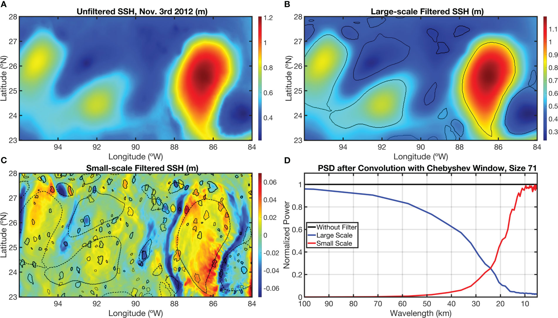
Figure 1 The SSH fields (m) in the central Gulf of Mexico for Nov. 3^rd, 2012, showcasing the filtering process and eddy detection methodologies. (A) The total scale model outputs; (B) the large scale filtered SSH after convolution with the Dolph-Chebyshev window and corresponding mesoscale eddy edge detections (black lines); (C) the small scale filtered SSH after subtracting (B) from (A) along with both detections of large and small scale eddies (black lines). (D) The normalized power spectrum for the large scale field (in blue) and the small scale field (in red) demonstrating a crossover point near 25 km.

2.3 Eddy detection and tracking

In order to detect eddy-like features, we employ an eddy detection and tracking algorithm first developed by Chaigneau et al, 2008; Chaigneau et al, 2009), expanded by Pegliasco et al. (2015), and employed by Trott et al, 2018; Trott et al, 2019), Roman-Stork et al, 2021; Roman-Stork et al, 2023), and Ernst et al. (2022). Notably for our purposes, this algorithm was also successfully used by Brokaw et al. (2020) to examine mesoscale eddy characteristics in the GoM. This algorithm detects eddies using closed contours of SSH. We use SSH instead of other fields (i.e. Vorticity or the Okubo-Weiss parameter) as SSH will provide the best comparison to forthcoming SWOT data, which is limited by noise effects such that only SSH will be effective below a 25 km resolution (Chelton et al., 2019; Chelton et al, 2022). Upon isolating local extrema in the SSH field (maxima for anticyclonic eddies and minima for cyclonic eddies), closed contours are drawn around them and expanded until the closed contour breaks, resulting in the final eddy edge detections laying upon the largest closed contours. This method does not require an arbitrary threshold for initial detection and results in a more accurate eddy shape than traditional thresholded methods.

Eddy trajectories over time are formed based upon a cost function that compares overlapping contours from adjacent time steps. Those overlapping closed contours that are minimally costed based upon radius, amplitude, and EKE are considered to be a part of the same trajectory. For more information on this cost function, see Pegliasco et al. (2015) or Trott et al. (2018). Given the hourly nature of the estimates used in this study, we discard any eddy trajectories that are not coherent over at least a 12 hour timespan. This helps reduce the likelihood of false instantaneous detections and retains features that are coherent in the Eulerian sense over at least this length of time.

For additional accuracy in the context of elongated false detections upon fronts, we apply a shape-constraining test that compares the length of the longest axis across the center (major axis) to the shortest axis across the center (minor axis) of each eddy. In this context, the ratio of the major axis to the minor axis determines the circularity of the eddy: a ratio of 1 indicates a perfect circle. We choose a cutoff ratio of 0.35, which helps eliminate most of the frontal structures and filaments within our results. This is broadly similar to the classic circularity test (see Kurian et al., 2011 for details) and achieves comparable results to their circularity threshold of 50% shape error, e.g. Figure 1C. The ratio test is significantly faster computationally than the circularity test over a high resolution domain given the simplicity of the calculation and the number of eddies detected versus the need to draw and compare a perfect circle to every contour.

Eddies are detected and tracked on both the large and small scale fields (see Figures 1B–C). Large scale eddies are hereafter referred to as ‘mesoscale’ eddies, while small scale eddy-like features are referred to as submesoscale eddy-like variabilities or SEVs. Large scale features are not tracked on the unfiltered field, as submesoscale variabilities can interrupt the formation of closed contours and falsely reduce or eliminate detections of eddy contours.

Given that these smaller scale features do not often have rotation velocities that exceed their translation velocities, it is unlikely that these can trap fluids for greater lengths of time. While they may still provide loci for particle attraction, deflection, and leakage, they are isolated through the filtering process, not prevalent in the total-scale, and as of yet lack observation from satellite altimetry, so we will not refer to SEVs as true coherent submesoscale vortices. In a physical sense, the process of SEV classification is meant to extract eddies with a predominant submesoscale signature. However, this will also include other persistent submesoscale circular structures. We address the most likely causes and classifications of SEVs in Section 4.1.

3 Results

3.1 Mean characteristics of SEVs

Before an understanding of the characteristics of SEVs internal to mesoscale eddies can be constructed, the general distributions of eddy properties must be noted. In this way, we may draw comparisons between the performance of the LLC4320 simulation and both observations and other operational models (Brokaw et al., 2020). In keeping with a comparison to established eddy characteristics in the GoM, we annotate the locations of eddy generation, called generation numbers, the locations of all eddy detections, eddy radius, eddy amplitude, and EKE (Figure 2).

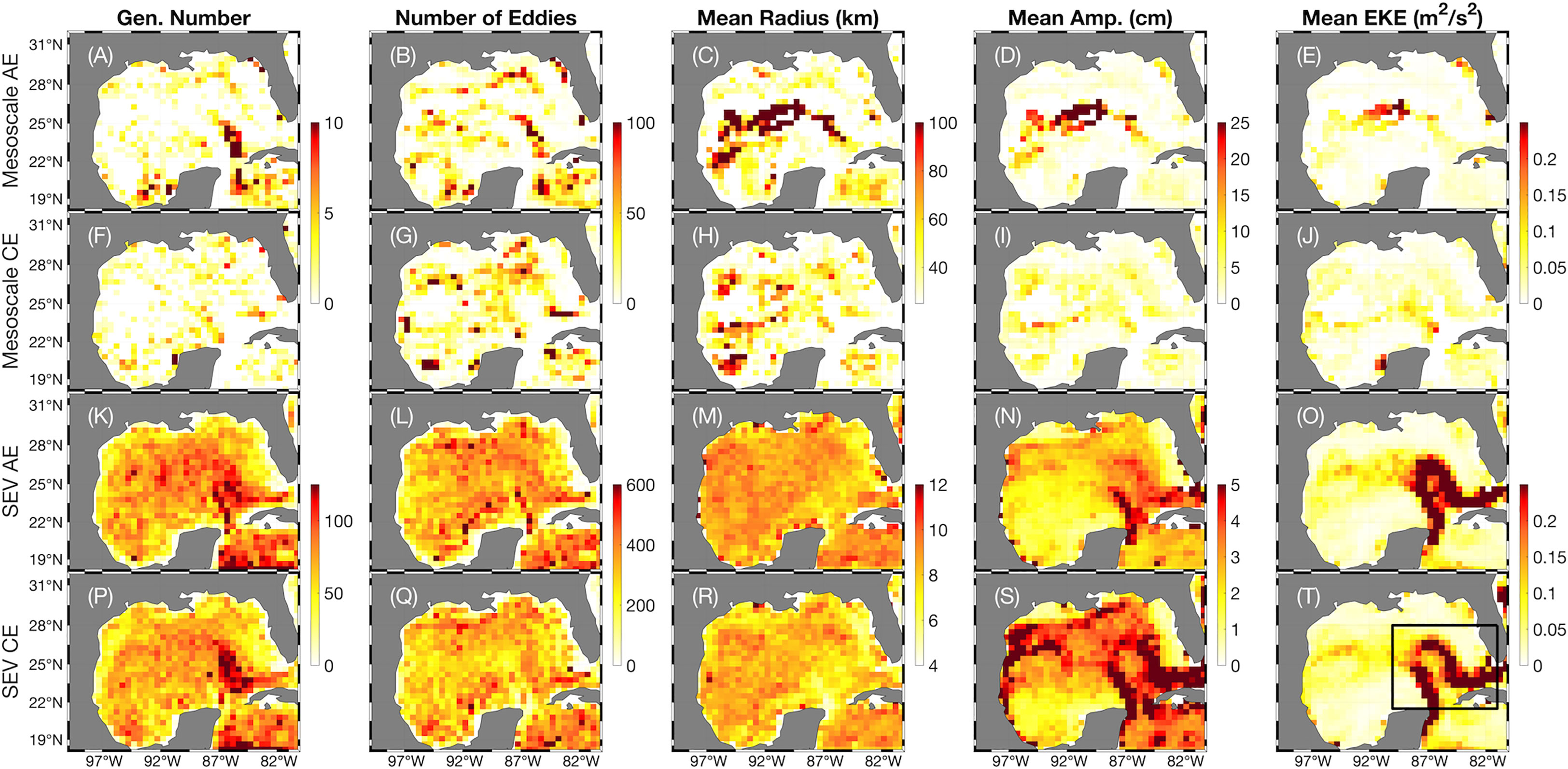
Figure 2 The properties of all mesoscale eddies and SEVs broken down geographically by eddy center location and binned into ½° pixels. (A–E) The generation number, i.e. number of eddies the originated in the pixel, the number of all eddy detections, the mean eddy radius (km), the mean eddy amplitude (cm), and the mean EKE (m² s^-2) for all mesoscale AEs. (F–J) As in (A–E) but for mesoscale CEs. (K–O) As in (A–E) but for SEV-AEs. (P–T) As in (A–E) but for SEV-CEs. The black box in (T) denotes the Loop Current region.

We find that the characteristics of the mesoscale-filtered eddies closely match those of both altimetry and the Hybrid Coordinate Ocean Model (HYCOM) as reported by Brokaw et al. (2020). There is a locus of eddy generation for Anticyclonic Eddies (AEs) in the extended Loop Current region (Figure 2A); these eddies propagate westward, with large radii (> 125 km), amplitudes (> 25 cm), and EKEs (> 0.2 m² s^-2) reported in the central to western GoM (Figures 2B–E). CEs, meanwhile, are less frequent and more prevalent throughout the basin’s edges (Figures 2F, G), with a notable persistently large CE in the southwest (Figure 2H). We find that our model does overestimate the EKE intensity of central GoM eddies as compared to observations, but that the relative distribution of properties is otherwise comparable.

The occurrences of SEVs, both AE and CE, are spread across the entire basin but are concentrated in the center and east with certain pixels of the Loop Current generating over 200 SEVs over the course of the 14-month simulation (Figures 2K, L, P, Q). SEV radii are near uniform, with the entire basin averaging 7-8 km (Figures 2M, R) while there is a trend for SEV amplitudes and EKEs to follow the path of the extended Loop Current and its LCEs (Figures 2N, O, S, T). High amplitudes and EKEs are also exhibited to the north of the LCE track and along the western coast of the GoM. It is worth noting that the areas of highest EKE intensity only outline the extended Loop Current and not its retracted state, mirroring the energy analysis of Loop Current instabilities conducted by Yang et al. (2020). Given that submesoscale eddies are often generated by such instabilities, it follows that SEVs would be observed along the Loop Current front (Buckingham et al., 2017). Beyond the geographic distribution of SEV characteristics, it is helpful to examine the timewise variability of SEVs over the 14-month duration of the simulation (Figure 3).

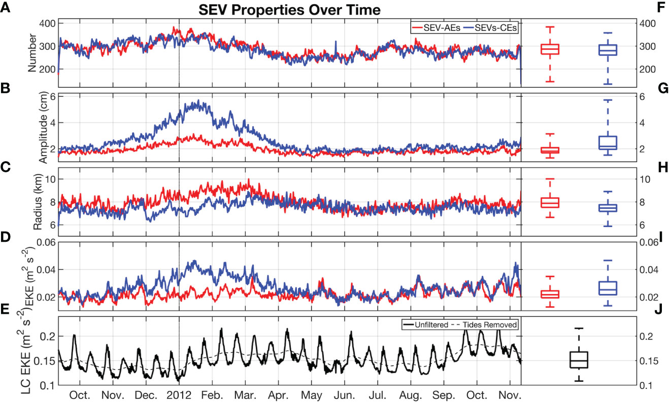
Figure 3 The properties of all SEVs over time from the beginning of the model simulation to its end, separated into AEs and CEs and binned into 12-hour increments. (A) The number of eddies per increment; (B) the median eddy amplitude (cm); (C) the median eddy radius (km); (D) the median eddy EKE (m² s^-2). (E) The EKE for the Loop Current region as defined by Brokaw et al. (2020): 21.5°N - 28°N and 81°W-90°W, both with and without tidal variability (as removed by a low-pass Gaussian filter with a half-window of 28 days). (F–J) As in (A–E) but using a box plot to show the median, quartiles, and extremes of the data upon which the time series is constructed.

The number of SEVs across the basin is relatively consistent, with a grouping around 280 SEVs of each rotational tendency per day (Figures 3A, F). That stated, there is some degree of variability present, with the highest number of SEVs observed in January (~320) and the lowest number in April-June (~250) before rising slightly (~280) to the end of the simulation. SEV amplitudes are consistently lower than those of mesoscale eddies at around 2 cm (calculated between the eddy center and contour, Figures 3B, G) which follows from the magnitude of the submesoscale filtered SSH field being roughly an order of magnitude less than the large-scale field (Figures 1B, C). Between the middle of October and the end of March, the amplitude and EKE of SEV-CEs nearly double those of SEV-AEs even as SEV-AE amplitude increases, while median SEV-CE radius actually declines below that of the median SEV-AE radius (Figures 3C, D, H, I). This is most likely due to the increase in instabilities caused during the generation and separation of a major LCE, as we discuss later.

Finally, we note that the EKE of the Loop Current itself follows a periodic pattern that matches with fortnightly tidal variability associated with neap and spring tides (Figures 3E, J). Once this variability is removed, it is clear that the EKE of the Loop Current reaches its greatest extents between February-May 2012 and September-November 2012. These coincide with the periods of greatest Loop Current extension during the simulation. To investigate how the intensity of the Loop Current and the tidal frequencies interact with the characteristics displayed in Figure 3, we perform a wavelet coherence analysis using the analytic Morlet wavelet (Figure 4, Grinsted et al., 2004).

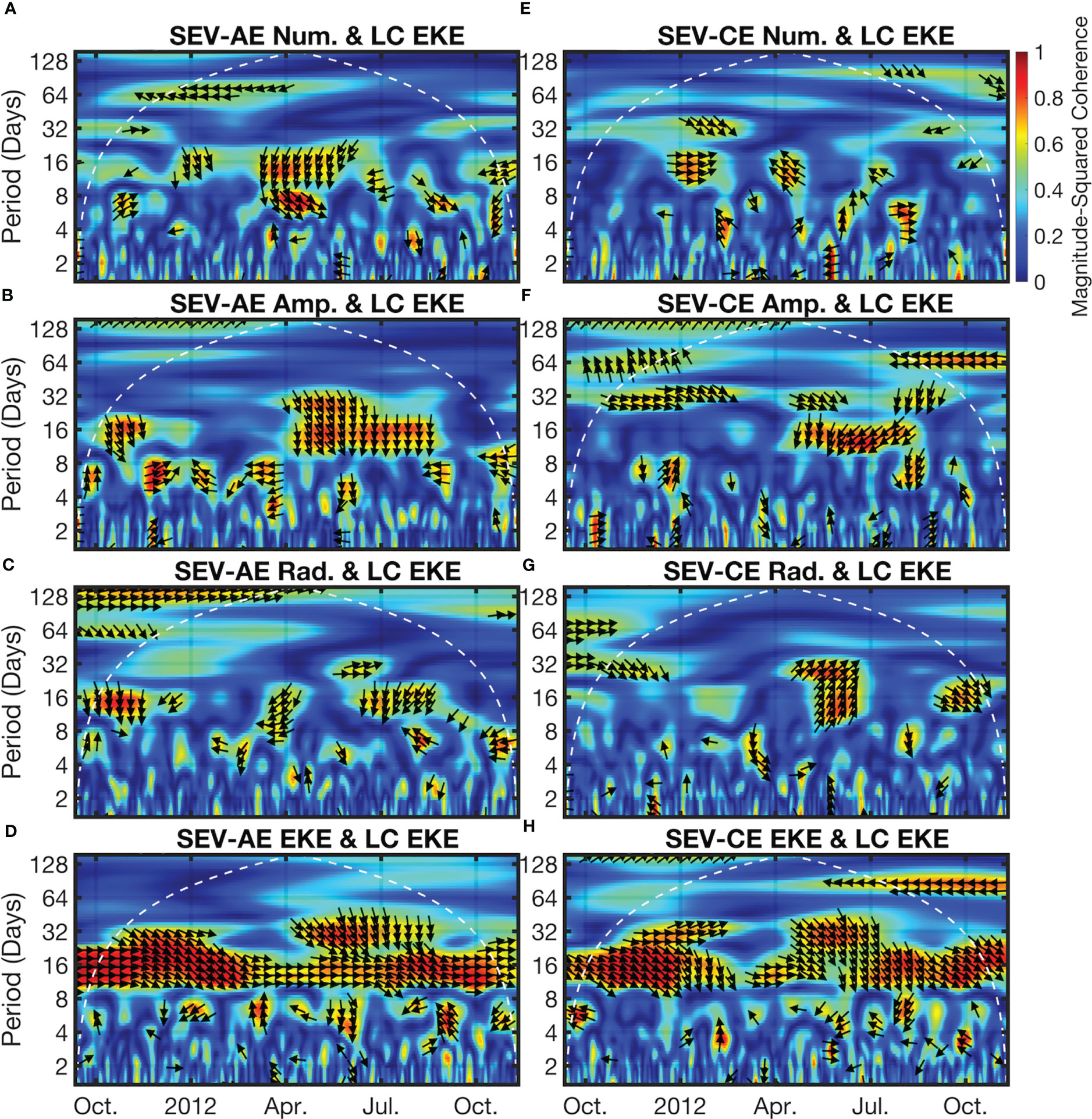
Figure 4 The magnitude-squared wavelet coherence computed using the analytic Morlet wavelet between each of the time series in Figures 3A-D, E. The white dashed line shows the cone of influence, after which edge effects dominate, while the black arrows show the direction of phase for coherence > 0.5. Rightward-facing arrows indicate the time series are in-phase, leftward facing arrows indicate the time series are anti-phase, downward facing arrows generally indicate that the first time series leads the second by 90 degrees, and upward facing arrows generally indicate that the second time series leads the first by 90 degrees. (A–D) The coherence between SEV-AEs number, amplitude, radius, and EKE time series and the Loop Current time series. (E–H) As in (A–D) but for SEV-CEs.

The primary period of coherence between the energetics of the Loop Current and the characteristics of SEVs occurs in the 10-20 day range, with some degree of significant coherence across all properties at some point during the simulation. Among the characteristics highlighted, amplitude and EKE are most frequently significant, with the EKE of the Loop Current and the EKE of SEV-AEs being persistently in phase (rightward pointing phase arrows) throughout the entire simulation. By contrast, the amplitudes of most SEVs, where notable, lie either slightly against phase or lagged by 90 degrees (downward pointing arrows). In this context, the most important implication is that the fortnightly tidal cycle is immediately influencing the EKE of SEVs.

3.2 Characteristics of internal SEVs

With the general properties of SEVs laid out in the previous section, we may turn our attention to the prospect of SEVs internal to mesoscale eddies. In this analysis, we collocate SEVs whose contours enclose an area that is within a ‘parent’ mesoscale eddy. There are therefore 4 combinations of SEVs and mesoscale eddies: SEV-AEs within mesoscale AEs (abbreviated M-AE where appropriate), SEV-CEs within M-AEs, SEV-AEs within mesoscale CEs (abbreviated M-CE where appropriate), and SEV-CEs within mesoscale CEs. Of the 54,330 SEV-AE trajectories identified, 8,958 (16.5%) contain at least one timestep where they are mostly within a mesoscale eddy; of the 54,951 SEV-CE trajectories identified, 7,346 (13.4%) contain at least one timestep where they are identified within a mesoscale eddy. Thus, around 85% of SEV trajectories belong outside mesoscale eddies. For mesoscale eddies, 1038 of the total 1266 (81.99%) of M-AEs contain at least one SEV internally during their lifetimes. For M-CEs, 622 of the 789 (78.83%) M-CEs identified contain at least one SEV internally. It is worth noting that of the ~20% of mesoscale eddies that do not contain an SEV at any point in their lifetimes, none of them have a lifetime of greater than 7 days, indicating that all long lived eddies are subject to SEV-based variability at some point in their lives. On average, internal SEV-AEs (CEs) live for 2.8 (2.5) days, spending an average of 1.8 (1.6) of those days within a mesoscale eddy and propagating an average of 14.3 (12.7) km away from their origin point. The longest lived internal SEV-AE (CE) lasts for 61.5 (96.0) days and propagates 245.6 (295.6) km away from its origin. The other mean characteristics of SEVs are given in Table 1.

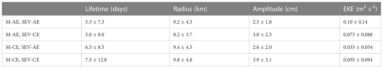
Table 1 The arithmetic means and standard deviations of Internal SEV lifetimes (column 1), radii (column 2), amplitudes (column 3), and EKE (column 4) for SEV-AEs internal to mesoscale AEs (row 1), SEV-CEs internal to mesoscale AEs (row 2), SEV-AEs internal to mesoscale CEs (row 3) and SEV-CEs internal to mesoscale CEs (row 4).

Overall, while there is substantial variance in all parameters, SEVs within M-CEs have the longest lives, SEVs within M-AEs have the highest EKEs, and SEV-CEs have greatest amplitudes. We break these characteristics down geographically in the same manner as all SEVs (Figure 5).

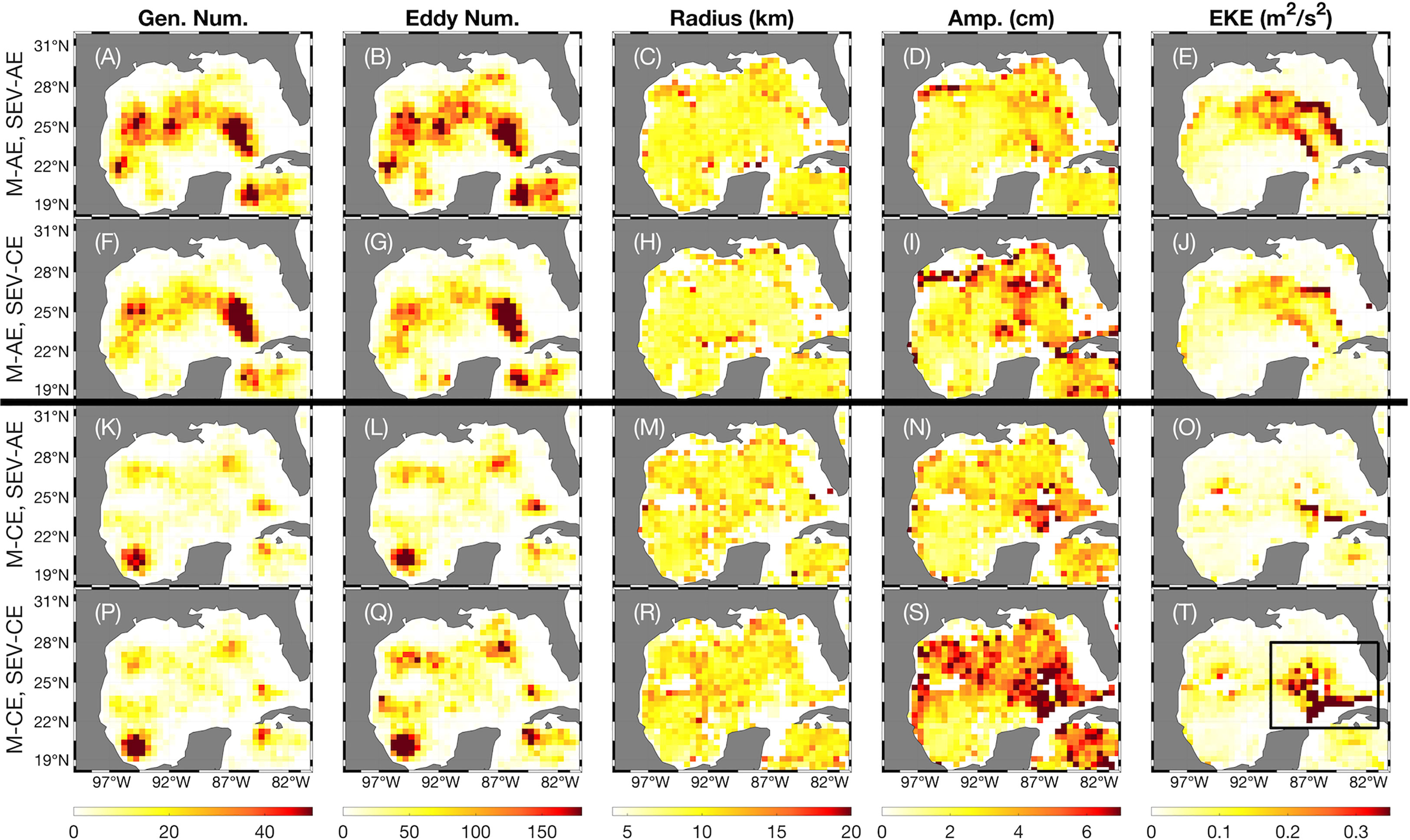
Figure 5 The geographic properties, as in Figure 2, for each type of internal SEV-outer mesoscale eddy combination pair. (A–E) The generation number, the mean eddy radius (km), the mean eddy amplitude (cm), and the mean EKE (m² s^-2) for all SEV-AEs internal to mesoscale AEs. (F–J) As in (A–E) but for SEV-CEs internal to mesoscale AEs. (K-O) As in (A–E) but for SEV-AEs internal to mesoscale CEs. (P–T) As in (A–E) but for SEV-CEs internal to mesoscale CEs. The black box in (T) denotes the Loop Current region.

We note that the geographic distribution of internal SEVs within M-AEs closely follows the track of LCEs (Figures 5A–B, F–G), with an additional increased concentration within the western Caribbean Sea. M-CE internal SEVs are most frequent within the southwestern corner of the GoM, corresponding to an intense, persistent M-CE (Figures 5K-L, P–Q). Three other loci of SEV-CE formation are notable: the eastern bend of the Loop Current, the tip of the extended Loop Current, and the northern Caribbean. As before, these all correspond to M-CE hotspots, both in our simulation (Figure 2) and in observations (Brokaw et al., 2020). Internal SEVs of all types on the boundaries are comparatively rare. This may be due in part to the filtering process, since results towards the boundaries are less reliable where there is insufficient data to fill the full filter window and so there are less mesoscale eddy detections. The distribution, then, of internal SEVs closely follows the areas of large parent eddy formation, an unsurprising result. The same trends are seen in the amplitude and EKE of internal SEVs, though it is notable that the most intense M-CE, SEV-CEs are found not in the extended Loop Current but at the base of the Loop Current, itself not a hotspot of M-CE EKE (Figure 5T). The properties of internal SEVs are further laid out over the duration of the dataset in Figure 6.

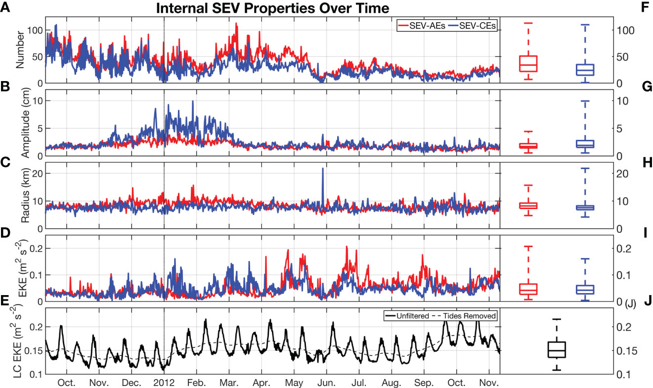
Figure 6 The time series of SEV properties, exactly as in Figure 3, but for only internal SEVs. Loop Current EKE is repeated without alterations. (A) The number of eddies per increment; (B) the median eddy amplitude (cm); (C) the median eddy radius (km); (D) the median eddy EKE (m² s^-2). (E) The EKE for the Loop Current region both with and without tidal variability. (F–J) As in (A–E) but using a box plot to show the median, quartiles, and extremes of the data upon which the time series is constructed.

We note a much more intense variability in the characteristics of internal SEVs as opposed to all SEVs, with the number of daily internal SEVs at one point dropping to just 4, causing the median radius spike at the end of May (Figures 6A, C). In contrast to Figure 3, there is also a prolonged period of time where internal SEV-AE numbers exceed those of SEV-CEs between the beginning of January and mid-May. After this point, the number of all internal SEVs never exceeds 50 of either type, despite having regularly exceeded this value previously. During this second half of the simulation, internal SEV-AE EKE rises, more often exceeding that of internal SEV-CEs. The increase in SEV-CE amplitude between December and March is also present here, though with more inherent variability (Figure 6B). As in Figure 4, we wish to determine whether there is significant coherence between the energy of the Loop Current and the energy of SEVs (Figure 7).

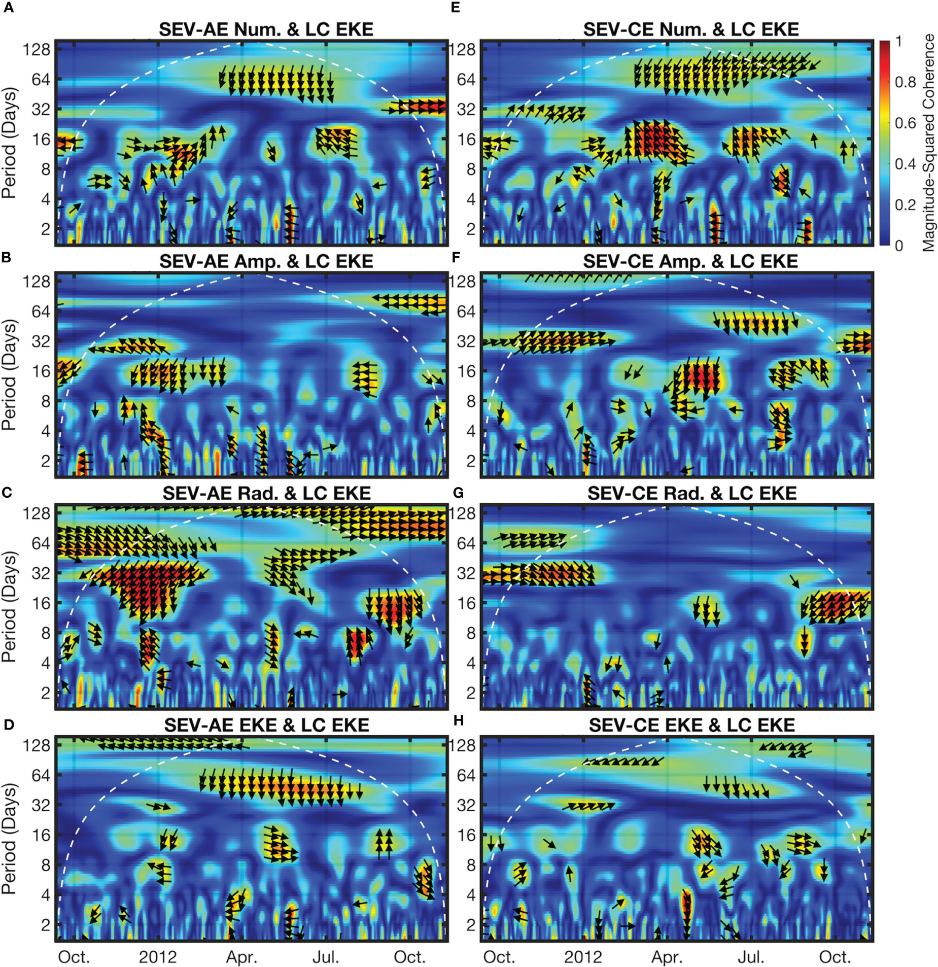
Figure 7 The Morlet wavelet coherence, exactly as in Figure 4, but for the internal SEV time series in Figure 6. The white dashed line shows the cone of influence, after which edge effects dominate, while the black arrows show the direction of phase for coherence > 0.5. (A–D) The coherence between internal SEV-AEs number, amplitude, radius, and EKE time series and the Loop Current time series. (E–H) As in (A–D) but for internal SEV-CEs.

While there is significant coherence at the 32-day period near the beginning of the simulation for all non-EKE characteristics, there is a distinct lack of coherence at the 16-day period for EKE as there was in Figure 4 (Figures 7D, H). Interestingly, there is a particularly strong coherence between internal SEV-CE number and the 16 day period between February and April, with the phase arrows showing both the number of SEV-CEs leading Loop Current EKE (upwards arrows) and the two being anti-phase. This is the only relation of all those seen in Figures 4, 7 that demonstrates a significant lead from SEV properties to Loop Current properties. This also partially coincides with the increase in SEV-CE amplitudes observed in Figures 3, 6, indicating a possible relationship between the generation of instabilities in the Loop Current and its strength. However, there is no significant coherence between internal SEV-CE amplitudes and Loop Current EKE at this time. With the general characteristics of internal SEVs established, we turn our attention to the relationship between the properties of parent mesoscale eddies and their internal SEVs (Figure 8).

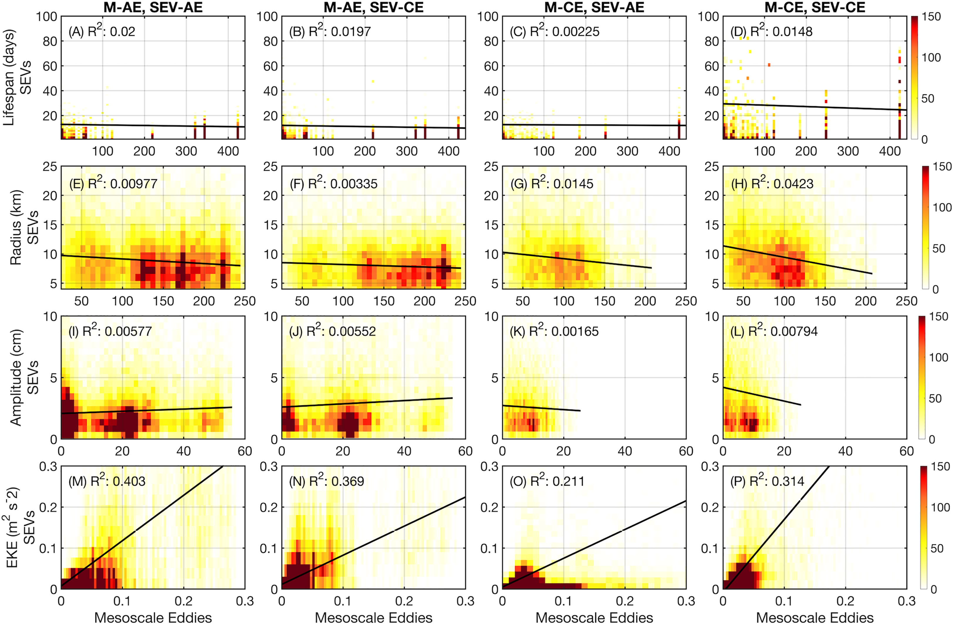
Figure 8 The binned histograms, in number of eddies, between the coincident properties of parent mesoscale eddies (x-axes) and their internal SEVs (y-axes) for each type of internal SEV-outer mesoscale eddy combination pair (columns 1-4). (A–D) The lifespans (days) of SEVs versus their parent mesoscale eddy lifespans. (E–H) The radii (km) of SEVs versus their parent mesoscale eddy radii. (I–L) The amplitudes (cm) of SEVs versus their parent mesoscale eddy amplitudes. (M–P) The EKEs (m² s^-2) of SEVs versus their parent mesoscale eddy EKEs. Linear regressions are shown as black lines with R² values annotated.

The lifespans of internal SEVs range between the minimum coherence interval (12 hours) and 80 days, with the longest-lived SEVs being those CEs internal to mesoscale CEs (Figures 8A–D). In particular, due to the length of the simulation, there are a handful of major mesoscale eddies that remain coherent for over half of the simulation, standing out clearly as sources of internal SEVs. There are in fact two mesoscale eddies whose lifespans cover the entirety of the simulation, one AE and one CE. The CE in particular is clearly visible in Figure 8D, as it contains a large number of long-lived internal SEVs. While some longer lived SEVs are present in shorter lived mesoscale eddies, demonstrating the capability for submesoscale structures to persist through the dissipation of a mesoscale eddy, all longer lived (lifespan > 10 days) SEVs whose trajectories are over 50% internal to mesoscale eddies are logically only found in longer-lived mesoscale eddies. The overall correlation between SEV and mesoscale eddy lifetimes is not significant (p < 0.05).

The same relationship does not hold true for radius (Figures 8E–H) or amplitude (Figures 8I–L), with the mean radius of SEVs (~8 km) remaining relatively constant for all radii of parent eddy with very low R² values on a slightly negative trend; trends for radius and amplitude are also not statistically significant. Amplitude for SEVs internal to M-AEs follows a dipolar pattern, with a grouping of SEVs in low-amplitude M-AEs (~5 cm) and another in high-amplitude M-AEs (~23 cm). By contrast, SEVs internal to M-CEs mostly cluster around 10 cm in the parent eddy, without a spike in SEV number at lower amplitudes. Finally, the relationship between SEV and mesoscale eddy EKE is mostly focused around the origin, with lower EKE mesoscale eddies unable to host SEVs of higher EKE, and the number of high-EKE SEVs peaking around a parent eddy mean EKE of around 0.03 m² s^-2 in all cases (Figures 8M–P). All correlations between SEV and mesoscale eddy EKEs are statistically significant. Another important element to examine in the relationship between mesoscale eddies and SEVs is how this relation changes over the course of the parent eddy lifetime (Figure 9).

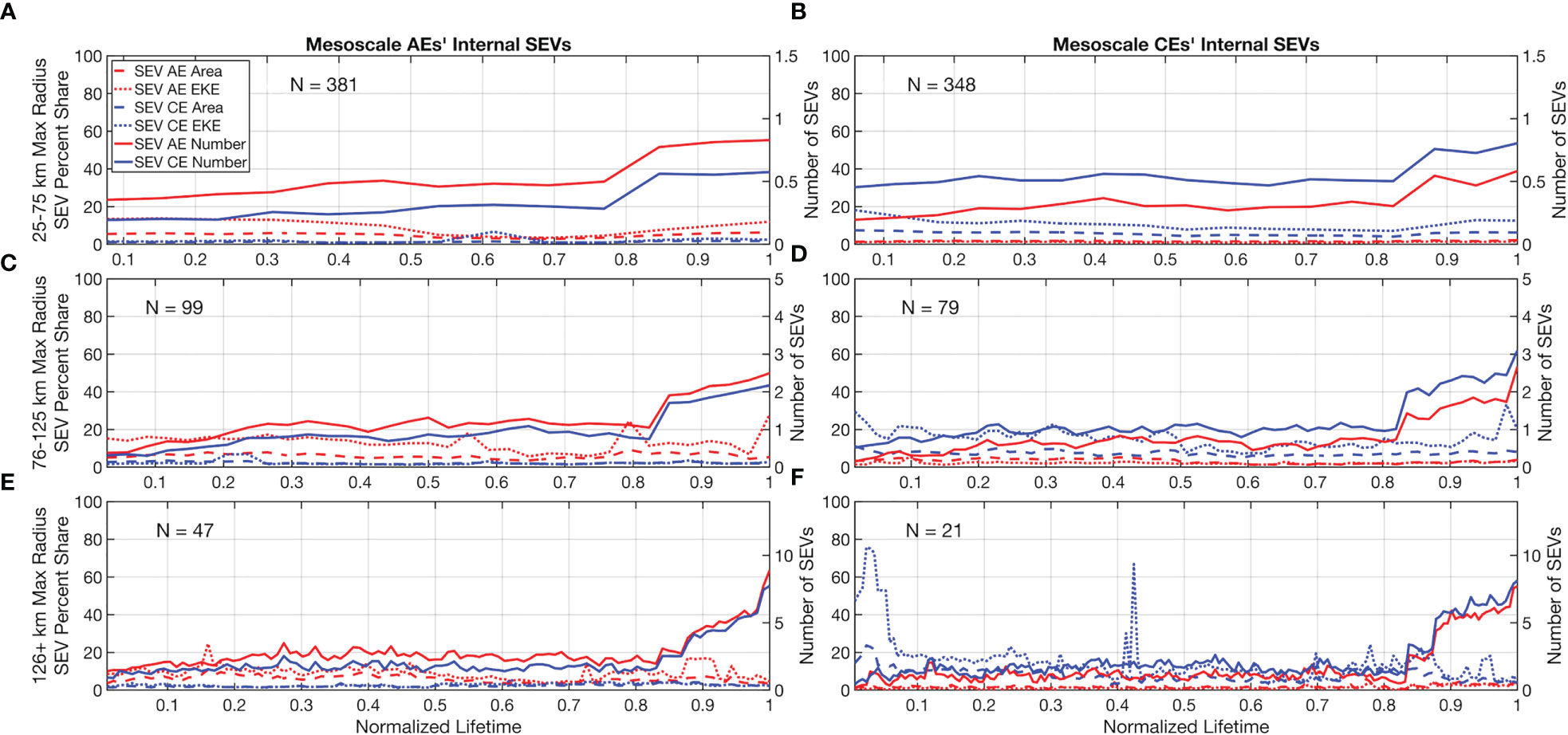
Figure 9 The numbers, fractions of parent eddy area, and fractions of parent eddy EKE taken up by internal SEVs over the normalized lifespan of their parent eddies. Number of parent eddies in each figure is shown. The left y-axes depict the percentage statistics, while the right y-axis depict the number of SEVs. (A) The statistics for parent AEs with a maximum trajectory radius of between 25 and 75 km. (B) As in (A) but for parent CEs. (C) As in (A) but for eddies whose maximum radius lies between 76 and 125 km. (D) As in (C) but for parent CEs. (E) As in (A) but for eddies whose maximum radius lies above 126 km. (F) As in (E) but for parent CEs.

Based upon the statistics of our mesoscale eddy detections, we separate the parent mesoscale eddies into classes based upon their maximum radii: 25-75 km covers eddies up until roughly the mean, 76-125 km covers eddies between 1 and 2 standard deviations above the mean, and 126+ km covers eddies with maximum radii above 2 standard deviations above the mean. For all sizes of mesoscale eddies, we catalogue the number of internal SEV-AEs and SEV-CEs along with the percent of the parent eddy that is taken up by the internal SEVs in both spatial area and EKE. We find in all sizes of mesoscale eddies that the number of internal SEVs begins to rise at around 80% through the parent eddy’s lifetime. Towards the end of an average large eddy lifetime, between 8 to 9 internal SEVs of each type are expected as the eddy decoheres (Figures 9E–F). The EKE and area shares only slightly increase during this time, without the same rapid increase. A notable exception is in mid-size M-CEs, where SEV-CE EKE share rises to 35% of the parent eddy total (Figure 9D).

In all cases, the same rotation direction between SEV and mesoscale eddy (CE-CE or AE-AE) is more likely to be found within an eddy, rather than the counterrotating opposite (CE-AE or AE-CE). Similarly, the EKE and area shares are dominated by same-direction rotating pairs, with an average value for same-direction pairs lying between 10 and 20% of the parent eddy, while opposite-direction pairs average between 0 and 10% for all eddy sizes. One last anomaly is in the lowest sample size category, large M-CEs: there are intense spikes in SEV-CE EKE share at the beginning and middle of the M-CE normalized lifetime (Figure 9F). Given that the figure shown is of an arithmetic mean, this is more likely to be contaminated by a handful of outliers; however, the values shown (76.7% at the beginning and 67.9% in the mid-life) are too high for a single outlier to be fully responsible. Additionally, we do see an early-life trend for higher SEV-CE EKE share in smaller M-CEs (Figures 9B, D). This indicates that there may be a relationship between M-CE and SEV-CE EKE in the formation stages in addition to death stages; this relationship is not present in M-AEs and SEV-AEs. While the previous figures have indicated the characteristics of SEVs inside of parent eddies, the probabilities of the locations of the SEVs have yet to be interrogated. We examine this distribution in Figure 10.

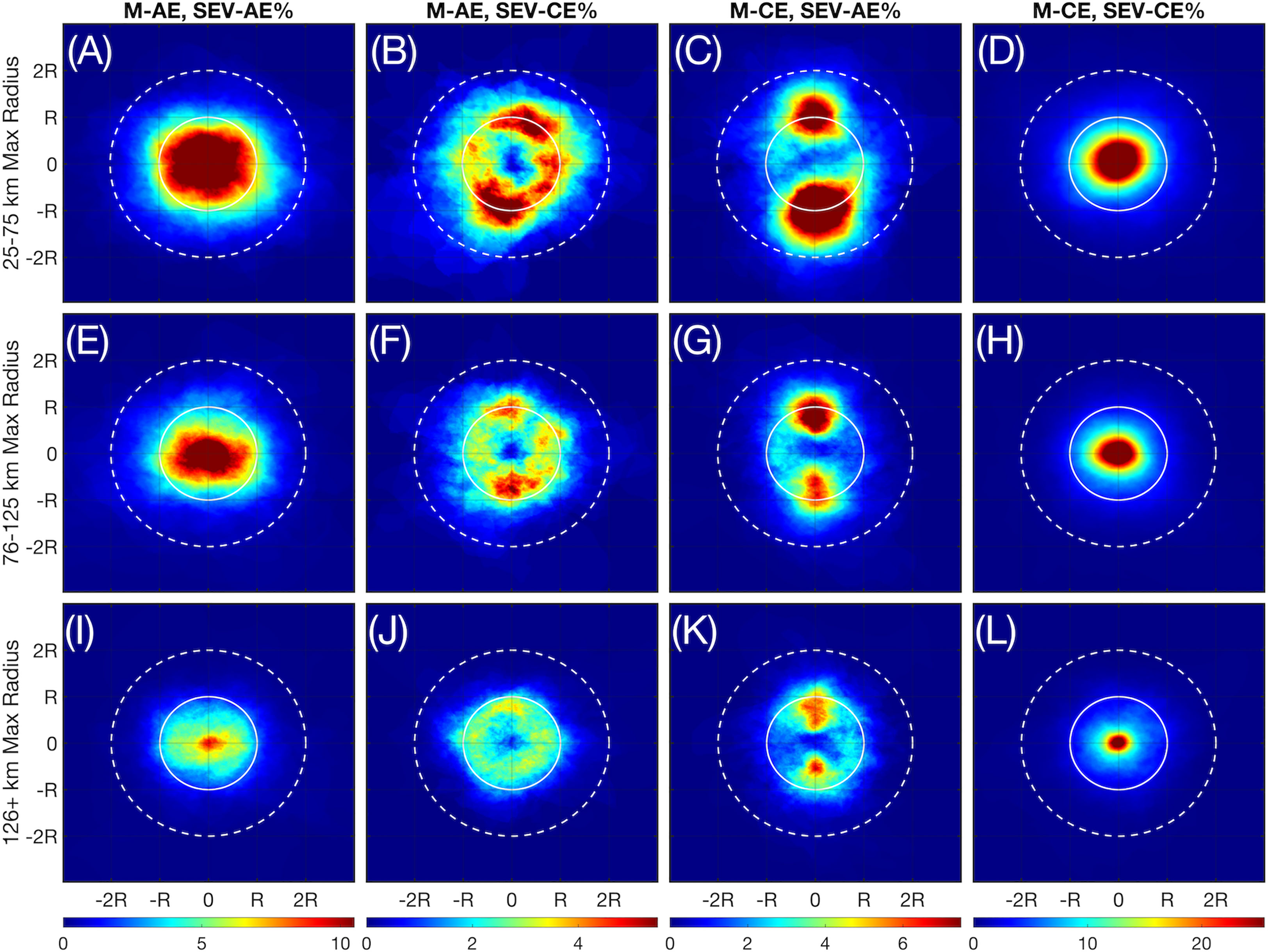
Figure 10 The locational composites for all instances of internal SEVs, showing the likelihood of a SEV covering a given pixel in a mesoscale eddy in percentage points for each type of internal SEV-outer mesoscale eddy combination pair. (A–D) The composites for eddies of maximum radius between 25 and 75 km. (E–H) As in (A–D) but for eddies of maximum radius between 76 and 125 km. (I–L) As in (A–D) but for eddies whose maximum radius lies above 126 km.

The rows of Figure 10 are broken down as in Figure 9 for eddies of increasing maximum radii. The greatest probability of SEV occurrence is for M-CEs and SEV-CEs, where there is over a 25% chance of finding an SEV-CE at any given timestep in the center of any given M-CE (Figures 10D, H, L). This likelihood decreases away from the center of the eddy until a minimum is reached beyond 1 radius of the M-CE. Given that the size of SEVs is relatively consistent between 6 and 12 km, while the size of mesoscale eddies varies considerably, it follows that the probabilities of SEVs in larger mesoscale eddies would take up less of the overall eddy in the composite. However, the overall shape of the pattern is the same. A similar pattern is observed for M-AEs and SEV-AEs, although the likelihood is halved and the distribution is flattened longitudinally (Figures 10A, E, I). Furthermore, the pattern for M-AEs is more diffuse, reaching beyond the first radius of the M-AE for smaller eddies. It also worth noting that some of the “SEVs” observed in the centers of same-type rotation pairs are actually the centers of the original mesoscale eddy leaking through the filter.

The more intriguing of the probability patterns are those found on opposite-type rotation pairs. While the most rare to find in one particular point in the eddy, M-AEs and SEV-CEs exhibit a ringed pattern focused on the edge of the first eddy radius, gradually shifting inside the radial edge as eddy size increases (Figures 10B, F, J). This is most intense on the northern and southern edges. In a similar way, M-CEs and SEV-AEs exhibit a stricter dipolar pattern with two loci to the direct north and south of the eddy center and lying once again on or slightly in from the first eddy radius (Figures 10C, G, K). Interestingly, smaller M-CEs have a larger focus of SEV-AE activity on their southern edge; however, this reverses for larger eddies, with a more intense focus of SEV-AEs on the northern edge. In both opposite-type pairs, the center of the eddy is the least likely location for an SEV to occur, with a probability close to 0. The impacts of SEVs on mesoscale eddies may be evaluated not only through their location within mesoscale eddies, but also with their temperature and salinity signatures at the surface. We begin with sea surface temperature anomalies (SSTAs) of SEVs, computed as the difference between the center SST and the mean SST out to a distance of 3 radii (Figure 11).

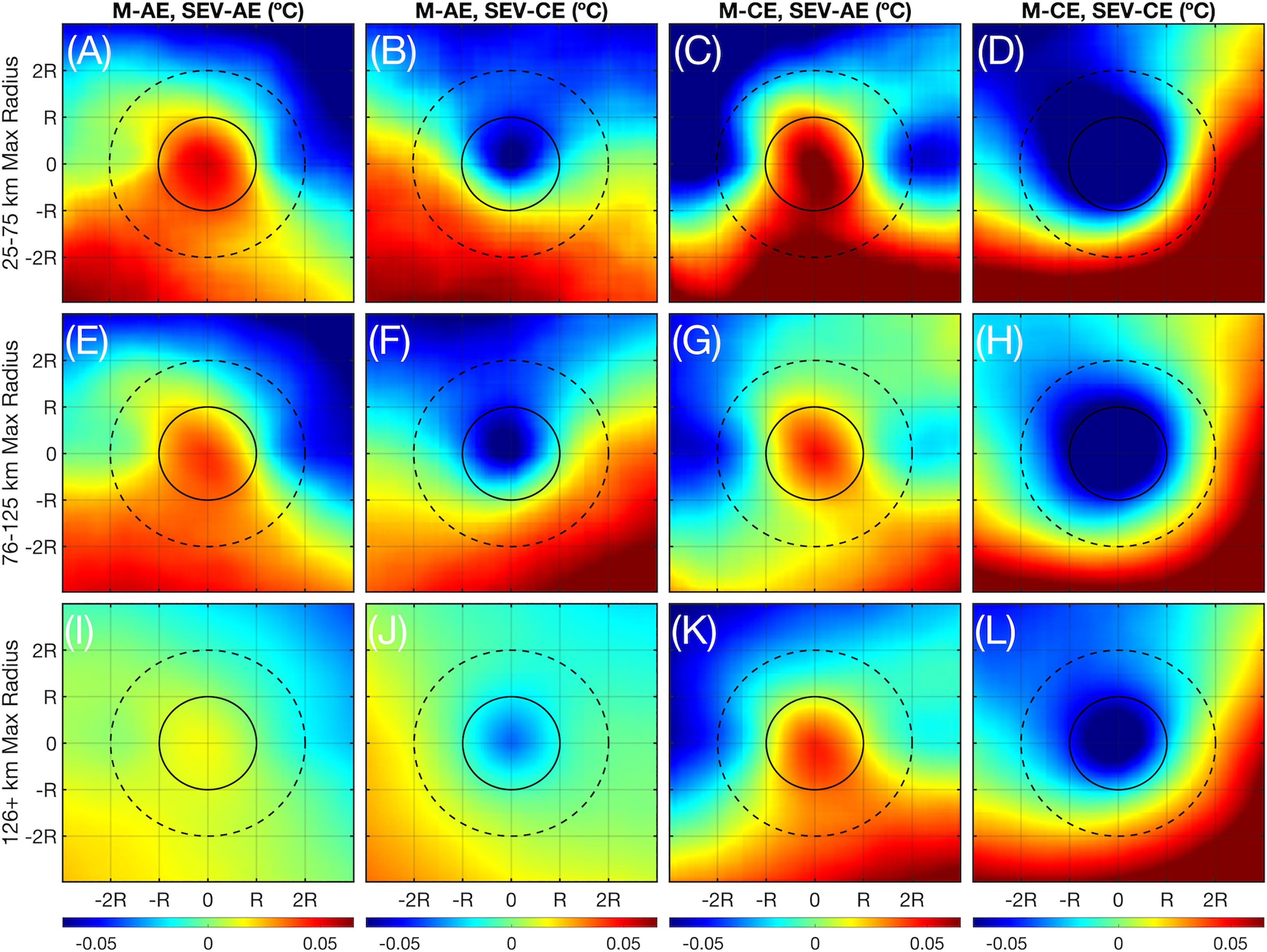
Figure 11 The composites for all SST anomalies (°C) associated with internal SEVs (difference between center SEV temperature and mean temperature computed up to 3 radii) for each type of internal SEV-outer mesoscale eddy combination pair. (A–D) The composites for eddies of maximum radius between 25 and 75 km. (E–H) As in (A–D) but for eddies of maximum radius between 76 and 125 km. (I–L) As in (A–D) but for eddies whose maximum radius lies above 126 km.

The general trend of the anomalies of the SEVs are as expected: the cyclonic, upwelling motion of SEV-Ces in all cases create a negative SSTA versus the background, while the anticyclonic, downwelling motion of SEV-AEs create a positive SSTA. This is most intense in the case of M-CEs, where SEV-AEs are associated with an SSTA of up to 0.06 °C and SEV-CEs are associated with an SSTA of up to -0.07 °C (Figures 11C, D, G, H, K, L). By contrast, the anomalies associated with M-AE internal SEVs are less intense but still present (Figures 11A, B, E, F, I, J). For all combinations, the anomalies are generally an order of magnitude less than those SSTAs associated with mesoscale eddies from observations (Brokaw et al., 2020). The general shape of the background SST is also comparable to those from observations, with a cooler flank generally to the north and a warmer flank to the south, attributable to the warmer Loop Current bringing warmer water to the south. As with SSTA, we compute the sea surface salinity anomalies (SSSAs) for SEVs of each type (Figure 12).

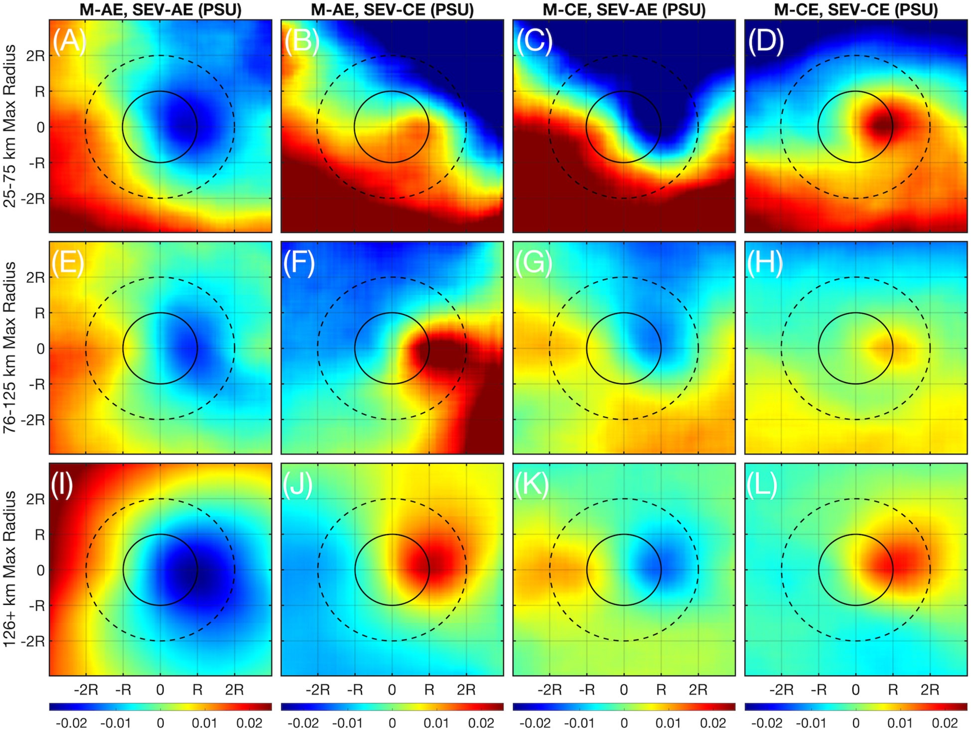
Figure 12 The composites for all SSS anomalies (PSU) associated with internal SEVs (difference between center SEV salinity and mean salinity computed up to 3 radii) for each type of internal SEV-outer mesoscale eddy combination pair. (A–D) The composites for eddies of maximum radius between 25 and 75 km. (E–H) As in (A–D) but for eddies of maximum radius between 76 and 125 km. (I–L) As in (A–D) but for eddies whose maximum radius lies above 126 km.

Interestingly, none of the SEVs exhibit a clear SSSA at their centers. Rather, each combination leads to a different arrangement of anomalies around the SEV center. In general, M-AEs and SEV-AEs lead to a negative SSSA to the direct east of the SEV center, being more intense with larger M-AEs (Figures 12A, E, I) while M-AEs and SEV-CEs demonstrate a positive SSSA to the east, with the most intense anomalies associated with mid-size eddies (Figures 12B, F, J). A similar set of patterns is exhibited for M-CEs and their constituent SEVs. However, the most intense SSSAs for M-CEs and both SEV-AEs and SEV-CEs is in smaller eddies rather than large ones (Figures 12C, D). While these patterns are similar in some respects to the patterns exhibited by observed mesoscale eddies in the GoM, such as the fact that the eddy center does not show a clear anomaly and that fresher water tends to originate to the north due to the Mississippi river outflow, the off-center anomaly is unusual (Brokaw et al., 2020).

As our results have indicated, internal SEVs are most often found within large eddies and induce anomalies in both SSTA and SSSA while they are present. Therefore, the last analysis we conduct is on the subject of the relationship between LCEs and SEVs using the major LCE of the simulation (Figure 13).

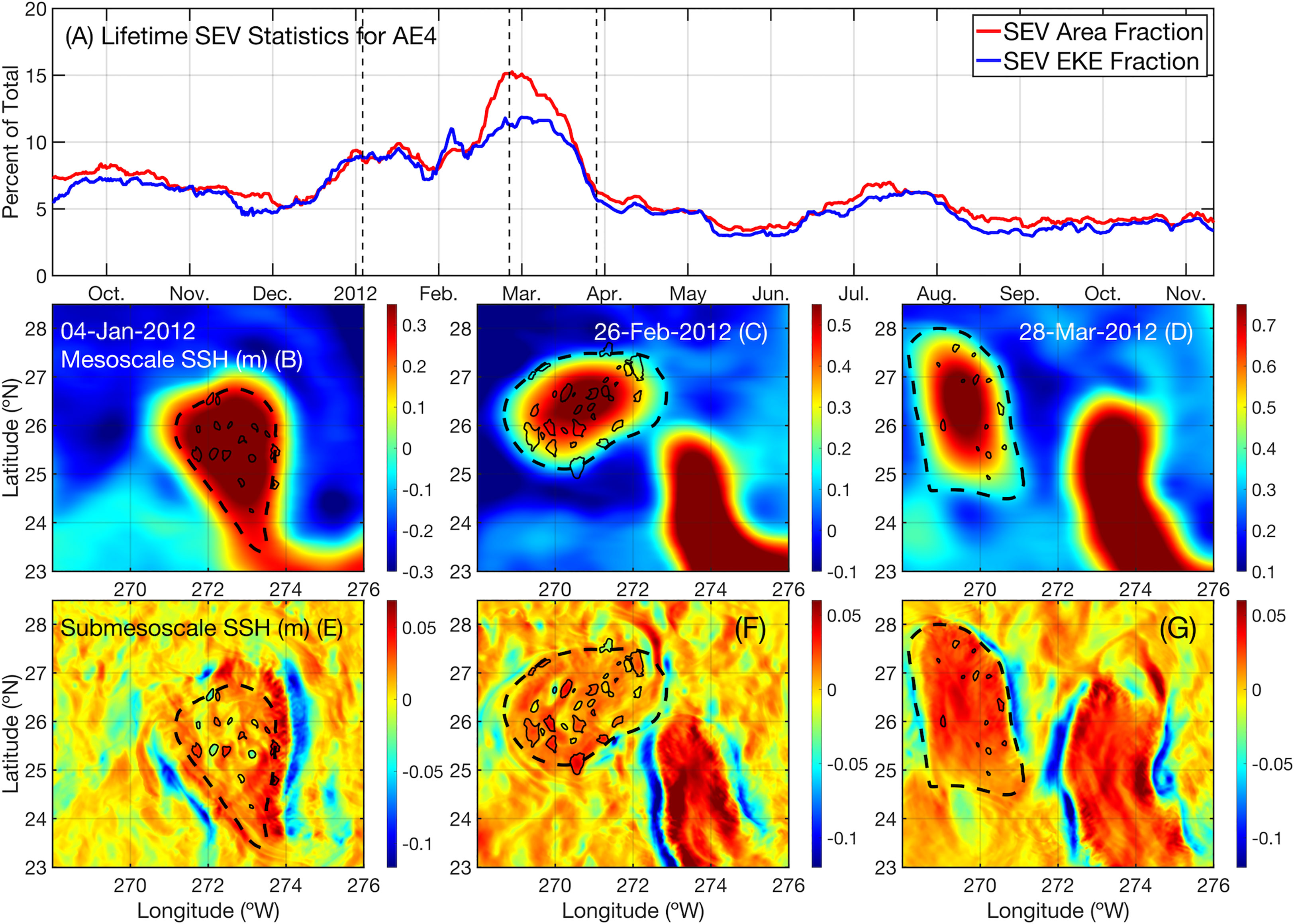
Figure 13 The separation of the Loop Current Eddy AE trajectory #4, or AE4. (A) The percent of AE4’s area and EKE taken up by SEVs over its lifespan, with black dashed lines showing the dates of the following snapshots. (B) The large-scale SSH (m) field associated with Jan. 4^th, 2012 showing AE4 (dashed line) and its internal SEVs (solid lines). (C) As in (B) but for Feb. 26^th, 2012. (D) As in (B) but for Mar. 28^th, 2012. (E–G) As in (B–D) but showing the small-scale SSH (m) field instead. .

This LCE is noteworthy for being identifiable from the beginning of the simulation (as the Loop Current begins in an extended state) all the way through the end, not actually dissipating during the duration of the simulation. It separates fully from the Loop Current in early February before propagating westward and resting on the western boundary. This particular LCE was the fourth AE identified by the eddy detection algorithm, and so is assigned the identifier AE4. Over the course of its life, AE4 always has at least 3 SEVs inside it, with at least 4% of its area and EKE devoted to these SEVs (Figure 13A). We showcase three snapshots of AE4 in relation to the Loop Current: one snapshot as the Loop Current is still extending in January (Figure 13B, E), one just after separation in late February (Figure 13C, F), and one a month after separating in late March (Figure 13D, G). As shown by the dashed lines in Figure 13A, these dates coincide with a middle, high, and low relative internal SEV composition respectively. We therefore observe that the SEVs reach a peak intensity inside AE4 just after separation from the Loop Current and rapidly fall thereafter as AE4 begins propagating westward.

4 Discussion

In our results we have emphasized the characteristics of SEVs and their relationships with mesoscale eddies. Generally, SEVs are short-lived (on the order of a week lifetime) structures that are ubiquitous in long-lived (longer than a week lifetime) mesoscale eddies. They are most concentrated in the Loop Current and in the LCEs that spawn from it, but their general characteristics are similar across all types of eddies. SEVs increase in number both in the splitting of LCEs from the Loop Current as well as towards the end of the lifetimes of mesoscale eddies. The amplitude of SEV-CEs in particular is a strong signal produced by an extending Loop Current about to shed an LCE (Figures 3B, 5B). The EKE of such SEVs strongly follows a fortnightly tidally induced signal apparent in the Loop Current. It is possible that, as suggested by previous literature, some of these SEVs are produced by barotropic tides near the coast (Callendar et al., 2011; Nakamura et al., 2012). Regardless of when they appear, SEVs induce submesoscale temperature and salinity variabilities in their parent mesoscale eddies. With this general breakdown, however, arises questions that we have not yet fully addressed in our analysis.

4.1 Proposed generation mechanisms of SEVs

We begin with an assessment of likely SEV generation mechanisms. One explanation particularly relevant for SEV-AEs, previously described by Brannigan (2016) and observed by Brannigan et al. (2017), is symmetric instabilities in the mixed layer. In this process, an instability is generated in the mixed layer, primarily driven by vertical buoyancy fluxes and vertical velocity shear, ultimately leading to a negative potential vorticity region at the surface. The number of filaments and structures generated through this process are shown to be highly resolution-dependent, first resolvable at the 2-km scale. As this is the scale resolved by our simulation, filaments, fronts, and eddy-like structures associated with symmetric instabilities may be associated with SEV-AEs found in the cores of M-AEs. Symmetric instabilities are also observed by de Marez et al., (2020b) to act at the northern edge of a simulated eddy, which then induces diapycnal mixing. Therefore, symmetric instabilities may explain the dipolar distribution of SEV-AEs within M-CEs. However, the coastal nature of the most numerous SEV-AEs within M-CEs (i.e. Figure 5K, L, P, Q) may also play a role in forcing this distribution. The intense vertical velocities associated with such structures, robust throughout studies of the submesoscale, may explain also the coherency of the SSTA observed in their cores (Figure 11).

Symmetric instabilities as a possible cause for SEV generation is also supported by the instability analysis of Lahaye and Zeitlin (2015), but alongside baroclinic and barotropic instabilities. The dominance of baroclinic and barotropic instabilities in the generation of submesoscale structures is likewise supported by the observations of Buckingham et al. (2017). Similarly, Yang et al. (2020) report that baroclinic instabilities play a particular role in the genesis of eddies in the Loop Current region. They also observe a mechanical energy transfer between mesoscale eddies and high frequency frontal eddies as a part of an inverse energy cascade, an observation similarly reported by Lazaneo et al. (2022). The presence of SEVs, aligning with those frontal eddies described by Yang et al. (2020) correlates with the splitting of the LCE from the Loop Current as described previously (Figure 13). Therefore, through both baroclinic instabilities and the ensuing frontogenesis (i.e. Garabato et al., 2022), the generation of SEVs may indicate an intensification of the inverse energy cascade; this most likely varies in conjunction with the forward energy cascade on a seasonal basis, as highlighted by Yang et al. (2021). The concept that the inverse energy cascade might be uniquely prevalent for internal SEVs is supported by the findings in our Figure 9, as SEVs increase in number the closer a mesoscale eddy is to decoherence. These SEVs, particularly those of opposite sign that gather on eddy boundaries, may also play a role similar to the submesoscale structures noted by Haza et al. (2016), causing leakage across eddy boundaries. An eddy with more such SEVs, therefore, can be expected to fracture from within due to baroclinic and barotropic instabilities at and below the mixed layer expressed as a part of same-rotation type SEVs. At the same time, such an eddy might be leaking fluid to without due to symmetric instabilities and frontogenesis expressed by opposite-rotation type SEVs, possibly in a process similar to that described by Barkan et al. (2019) and Verma et al. (2019). The non-baroclinic processes are likely intensified as a mesoscale eddy approaches topographic features (Rosso et al., 2015; Morvan et al., 2019; Morvan et al., 2020). Lastly, it is worth noting that based upon the season and location of SEV formation the motions and predominant EKE that characterize SEVs may be either primarily balanced or unbalanced in terms of dissipation vs. atmospheric forcings; the reader is referred to Cao et al. (2023) for a more complete discussion on the nature of such motions as manifested in our model simulations.

4.2 SSSA anomaly patterns

While the SSTA patterns described in Figure 11 match those ascribed both to mesoscale eddies in the GoM and the dynamics of submesoscale vertical heat transport, the dynamical meaning behind the SSSA patterns of Figure 12 are less clear (Brokaw et al., 2020; Wang et al., 2022). As previously noted, in fact, the observed patterns are opposite of those expected in such structures from a theoretical standpoint. The SSSA signature associated with AEs is typically associated with an increased surface salinity, while the surface expression of CEs is more often associated with a decrease in surface salinity as described in mesoscale eddies throughout the world’s oceans (Melnichenko et al., 2017). The patterns seen in Figure 12, however, show an opposite effect, as SEV-AEs are associated with more intense freshwater anomalies and SEV-CEs are associated with more intense salinity anomalies. In both cases, the dipolar structure is expected, but the intensity of the poles are reversed.

The answer may be found in the work of Zhang et al. (2019). In this study, the formation of a submesoscale eddy is observed as a result of baroclinic instability in a slumping salinity front. The authors find that, due to the fresher surface layer, upwelling induced by the eddy resulted in a more saline surface layer. In the same fashion, large submesoscale salinity variations on the order of 0.05 psu at the surface as observed by Drushka et al. (2019) might be expected in the GoM due to the river plume of the Mississippi river. In effect, the decidedly fresher surface water of the GoM, especially towards its northern edge, is likely entrained by SEV-AEs, decreasing salinity adjacent to the SEV core. At the same time, SEV-CEs are responsible for upwelling through the surface layer, allowing for a more saline surface. This allows for frontal compensation across the GoM as described for freshwater-influenced regions by Spiro Jaeger and Mahadevan (2018). An intriguing connection here is made by Kobashi and Hetland (2020): the Mississippi river outflow is partially controlled by anthropogenic factors and remote interannual variabilities, e.g. the El Niño Southern Oscillation. As a result, SEVs and other structures often associated with salinity fronts may introduce an element of remote forcing into SEV variability. However, as the authors conclude, there is as of yet insufficient evidence to prove a significant link exists, especially at the under observed submesoscale.

4.3 Broader implications

The ubiquity of SEVs in the GoM and mesoscale eddies suggests that SEVs may play an important role in the biogeochemical cycling and chlorophyll dispersal within the Gulf. For example, frontal eddy structures have already been observed in the Florida Straits using ocean color data (Zhang et al., 2019). At the same time, mesoscale eddies in the Gulf have been shown to aid in the dispersal of chlorophyll-a as eddies interact and break plumes apart (Toner et al., 2003). SEVs and the frontal dynamics associated with them likely play a role in the advection and vertical movement of nutrients into and away from the surface layer, influencing the distribution of phytoplankton blooms and hypoxic zones (Rabalais et al., 2002). Internal SEVs and leakage associated with them may also complicate the transport of freshwater away from the river plume with future implications for the spread of pollutants (Özgökmen et al., 2016).

Another implication of SEV-induced variability in the Gulf is that on tropical cyclone strength. Warm sea surface temperatures associated with mesoscale eddies have been observed to correlate with an increase in storm strength (Jaimes et al., 2016). LCEs have also been drained of heat and forcibly dissipated through air-sea interactions with hurricanes (Potter et al., 2021). As we demonstrate here, the submesoscale variability of both the Loop Current and LCEs changes dramatically depending on life cycle stage. Future observations will serve to clarify the role that submesoscale oceanic variability plays in the intensification and feedbacks associated with hurricane growth.

Finally, machine learning based approaches have already demonstrated skill in the prediction of the separation of LCEs (Wang et al., 2019). The most prevalent of these approaches utilizes high resolution SSH time series to extract hidden patterns that lead to LCE separation spatiotemporal predictions. Greater resolution data and an increased understanding of the submesoscale dynamics within that data may improve the accuracy and skill of future predictions, as the separation of an LCE from the Loop current involves interactions across both the mesoscale and submesoscale that cannot be properly discerned from previously available data (Yang et al., 2020).

5 Conclusion

In this study, we have used a tailor-made filtering approach to efficiently separate the spatial scales in a high resolution modelling simulation. Through the use of an automated eddy detection and tracking algorithm, we have identified regions that, through shape, persistence, and SSH anomalies, behave like eddies. These so-called SEVs were then evaluated both across the entire spatiotemporal domain and in the context of mesoscale eddies, where SEVs were collocated within mesoscale eddy contours. To our knowledge, this is the first time this has been done algorithmically on a basin-wide scale. Through describing the characteristics of SEVs, particularly those internal to mesoscale eddies, we demonstrate that SEVs are typically responsible for up to 15% of the internal variability in terms of EKE, SSS, SST, and SSH in mesoscale eddies of all sizes throughout the GoM. We show that SEVs also correlate with the extensions of the Loop Current, with the number of SEVs internal to an LCE reaching a maximum just after separation from the loop current occurs. These findings have implications for biogeochemical processes in the Gulf, as well as Loop Current and LCE separation forecasting. Given our results’ dependence on our model’s resolution as demonstrated by previous studies, further observations are required to validate and confirm them. The SWOT mission, already in orbit and undergoing calibration and validation, promises to provide the first wide-scale SSH measurements of an effective resolution capable of resolving these SEVs.

Data availability statement

Publicly available datasets were analyzed in this study. This data can be found here: The National Aeronautics and Space Administration (NASA) Estimating the Circulation & Climate of the Ocean (ECCO) Data Portal, https://data.nas.nasa.gov/ecco/data.php?dir=/eccodata/llc_4320 .

Author contributions

BS managed the computational resources, funding acquisition, and lab space. All authors contributed to the conceptualization and design of the study. PE managed the data and wrote the software. All authors contributed to the formulation of the analysis. PE wrote the original draft of the manuscript. All authors contributed to the manuscript revision. All authors contributed to the article and approved the submitted version.

Funding

Research reported in this manuscript was supported by the Gulf Research Program of the National Academies of Sciences, Engineering, and Medicine under award #2000013149. The content is solely the responsibility of the authors and does not necessarily represent the official views of the Gulf Research Program or the National Academies of Sciences, Engineering, and Medicine. PE was funded by the U.S. Department of Defense Science, Mathematics, and Research for Transformation (SMART) Scholarship and the University of South Carolina Presidential Fellowship.

Acknowledgments

This has NRL contribution number NRL-JA-7320-23-5876. Approved for public release, distribution is unlimited. We thank the editor and three reviewers for their suggestions that significantly improved the quality of the final work.

Conflict of interest

The authors declare that the research was conducted in the absence of any commercial or financial relationships that could be construed as a potential conflict of interest.

The handling editor SM declared a shared consortium GOFFISH with the author BS at the time of review.

Publisher’s note

All claims expressed in this article are solely those of the authors and do not necessarily represent those of their affiliated organizations, or those of the publisher, the editors and the reviewers. Any product that may be evaluated in this article, or claim that may be made by its manufacturer, is not guaranteed or endorsed by the publisher.

References

Adcroft A., Hill C., Campin J.-M., Marshall J., Heimbach P. (2004). “Overview of the formulation and numerics of the MIT GCM,” in Proceedings of the ECMWF seminar series on numerical methods, recent developments in numerical methods for atmosphere and ocean modeling (ECMWF: Shinfield Park, Reading).
Arbic B. K., Elipot S., Brasch J. M., Menemenlis D., Ponte AurélienL., Shriver J. F., et al. (2022). Near-surface oceanic kinetic energy distributions from drifter observations and numerical models. J. Geophysical Research: Oceans 10, e2022JC018551. doi: 10.1029/2022JC018551
Barkan R. M., Molemaker J., Srinivasan K., McWilliams J. C., D’Asaro E. A. (2019). The role of horizontal divergence in submesoscale frontogenesis. J. Phys. Oceanography 6, 1593–1618. doi: 10.1175/JPO-D-18-0162.1
Bracco A., Liu G., Sun D. (2019). Mesoscale-submesoscale interactions in the gulf of Mexico: from oil dispersion to climate. Chaos Solitons Fractals 119, 63–72. doi: 10.1016/j.chaos.2018.12.012
Brannigan L. (2016). “Intense submesoscale upwelling in anticyclonic eddies.”Geophysical Res. Lett. 43, 3360–3369. doi: 10.1002/2016GL067926
Brannigan L., Marshall D. P., Naveira A. C., Garabato A. J., Nurser G., Kaiser J. (2017). Submesoscale instabilities in mesoscale eddies. J. Phys. Oceanography 12, 3061–3085. doi: 10.1175/JPO-D-16-0178.1
Brokaw R. J., Subrahmanyam B., Trott C. B., Chaigneau A. (2020). Eddy surface characteristics and vertical structure in the gulf of Mexico from satellite observations and model simulations. J. Geophysical Research: Oceans 2, e2019JC015538. doi: 10.1029/2019JC015538
Buckingham C. E., Khaleel Z., Lazar A., Martin A. P., Allen J. T., Naveira Garabato A. C., et al. (2017). Testing munk’s hypothesis for submesoscale eddy generation using observations in the north Atlantic. J. Geophysical Research: Oceans 8, 6725–6745. doi: 10.1002/2017JC012910
Callendar W., Klymak J. M., Foreman M. G. G. (2011). Tidal generation of Large Sub-mesoscale eddy dipoles. Ocean Sci. 4, 487–502. doi: 10.5194/os-7-487-2011
Cao H., Fox-Kemper B., Jing Z. (2021). Submesoscale eddies in the upper ocean of the kuroshio extension from high-resolution simulation: energy budget. J. Phys. Oceanography 7, 2181–2201. doi: 10.1175/JPO-D-20-0267.1
Cao H., Fox-Kemper B., Jing Z., Song X., Liu Y. (2023). Towards the upper-ocean unbalanced submesoscale motions in the oleander observations. J. Phys. Oceanography 4, 1123–1138. doi: 10.1175/JPO-D-22-0134.1
Chaigneau A., Eldin Gérard, Dewitte B. (2009). Eddy activity in the four major upwelling systems from satellite altimetr–2007). Prog. Oceanography Eastern Boundary Upwelling Ecosystems: Integr. Comp. Approaches 1, 117–123. doi: 10.1016/j.pocean.2009.07.012
Chaigneau A., Gizolme A., Grados C. (2008). Mesoscale eddies off Peru in altimeter records: identification algorithms and eddy spatio-temporal patterns. Prog. Oceanography Northern Humboldt Curr. System: Ocean Dynamics Ecosystem Processes Fisheries 2, 106–119. doi: 10.1016/j.pocean.2008.10.013
Chelton D. B., Samelson R. M., Farrar J.T. (2022). The effects of uncorrelated measurement noise on SWOT estimates of Sea surface height, velocity, and vorticity. J. Atmospheric Oceanic Technol. 7, 1053–1083. doi: 10.1175/JTECH-D-21-0167.1
Chelton D. B., Schlax M. G., Samelson R. M., Farrar J.T., Jeroen Molemaker M., McWilliams J. C., et al. (2019). Prospects for future satellite estimation of small-scale variability of ocean surface velocity and vorticity. Prog. Oceanography 173, 256–350. doi: 10.1016/j.pocean.2018.10.012
Chereskin T. K., Rocha C. B., Gille S. T., Menemenlis D., Passaro M. (2019). Characterizing the transition from balanced to unbalanced motions in the southern California current. J. Geophysical Research: Oceans 3, 2088–2109. doi: 10.1029/2018JC014583
D’Addezio J. M., Jacobs G. A., Yaremchuk M., Souopgui I. (2020). Submesoscale eddy vertical covariances and dynamical constraints from high-resolution numerical simulations. J. Phys. Oceanography 4, 1087–1115. doi: 10.1175/JPO-D-19-0100.1
de Marez C., Carton X., Corréard Stéphanie, L’Hégaret P., Morvan M. (2020a). Observations of a deep submesoscale cyclonic vortex in the Arabian Sea. Geophysical Res. Lett. 13, e2020GL087881. doi: 10.1029/2020GL087881
de Marez C., Meunier T., Morvan M., L’Hégaret P., Carton X. (2020b). Study of the stability of a Large realistic cyclonic eddy. Ocean Model. 146, 101540. doi: 10.1016/j.ocemod.2019.101540
Drushka K., Asher W. E., Sprintall J., Gille S. T., Hoang C. (2019). Global patterns of submesoscale surface salinity variability. J. Phys. Oceanography 7, 1669–1685. doi: 10.1175/JPO-D-19-0018.1
Durand M., Fu L.-L., Lettenmaier D. P., Alsdorf D. E., Rodriguez E., Esteban-Fernandez D. (2010). The surface water and ocean topography mission: observing terrestrial surface water and oceanic submesoscale eddies. Proc. IEEE 5, 766–779. doi: 10.1109/JPROC.2010.2043031
Ernst P. A., Subrahmanyam B., Trott C. B. (2022). Lakshadweep High propagation and impacts on the Somali current and eddies during the southwest monsoon. J. Geophysical Research: Oceans 3, e2021JC018089. doi: 10.1029/2021JC018089
Forget G., Campin J.-M., Heimbach P., Hill C. N., Ponte R. M., Wunsch C. (2015). ECCO version 4: an integrated framework for non-linear inverse modeling and global ocean state estimation. Geoscientific Model. Dev. 10, 3071–3104. doi: 10.5194/gmd-8-3071-2015
Fu L.-L., Christensen E. J., Yamarone C. A. Jr., Lefebvre M., Ménard Y., Dorrer M., et al. (1994). TOPEX/POSEIDON mission overview. J. Geophysical Research: Oceans 99, 24369–24381. doi: 10.1029/94JC01761
Garabato A. C.N., Yu X., Callies Jörn, Barkan R., Polzin K. L., Frajka-Williams E. E., et al. (2022). Kinetic energy transfers between mesoscale and submesoscale motions in the open ocean’s upper layers. J. Phys. Oceanography 52, 75–97. doi: 10.1175/JPO-D-21-0099.1
Grinsted A., Moore J. C., Jevrejeva S. (2004). Application of the cross wavelet transform and wavelet coherence to geophysical time series. Nonlinear Processes Geophysics 11, 561–566. doi: 10.5194/npg-11-561-2004
Gula J., Blacic T. M., Todd R. E. (2019). Submesoscale coherent vortices in the gulf stream. Geophysical Res. Lett. 5, 2704–2714. doi: 10.1029/2019GL081919
Haza A. C., Özgökmen T. M., Hogan P. (2016). Impact of submesoscales on surface material distribution in a gulf of Mexico mesoscale eddy. Ocean Model. 107, 28–47. doi: 10.1016/j.ocemod.2016.10.002
Jaimes B., Shay L. K., Brewster J. K. (2016). Observed air-Sea interactions in tropical cyclone Isaac over loop current mesoscale eddy features. Dynamics Atmospheres Oceans Loop Curr. Dynamics Experiment 76, 306–324. doi: 10.1016/j.dynatmoce.2016.03.001
Kobashi D., Hetland R. (2020). Reproducibility and variability of submesoscale frontal eddies on a broad, low-energy shelf of freshwater influence. Ocean Dynamics 70, 1377–1395. doi: 10.1007/s10236-020-01401-4
Kurian J., Colas F., Capet X., McWilliams J. C., Chelton D. B. (2011). Eddy properties in the California current system. J. Geophysical Research: Oceans 116. doi: 10.1029/2010JC006895
Lahaye Noé, Zeitlin V. (2015). Centrifugal, barotropic and baroclinic instabilities of isolated ageostrophic anticyclones in the two-layer rotating shallow water model and their nonlinear saturation. J. Fluid Mechanics 762, 5–34. doi: 10.1017/jfm.2014.631
Lazaneo C. Z., Calil P. H. R., Tandon A., da Silveira I. C. A. (2022). Submesoscale coherent vortices in the south Atlantic ocean: a pathway for energy dissipation. J. Geophysical Research: Oceans 127, e2020JC017099. doi: 10.1029/2020JC017099
Leben R. R., Born G. H. (1993). Tracking loop current eddies with satellite altimetry. Adv. Space Res. 13, 325–333. doi: 10.1016/0273-1177(93)90235-4
Liu X., Wang M., Wei S. (2009). A study of a hurricane Katrina–induced phytoplankton bloom using satellite observations and model simulations. J. Geophysical Research: Oceans 114. doi: 10.1029/2008JC004934
Liu Y., Weisberg R. H., Hu C., Kovach C., Riethmüller R. (2011). “Evolution of the loop current system during the deepwater horizon oil spill event as observed with drifters and satellites,” in Geophysical monograph series, vol. 195 . Eds. Liu Y., MacFadyen A., Ji Z.-G., Weisberg R. H. (Washington, D. C: American Geophysical Union), 91–101. doi: 10.1029/2011GM001127
Lynch P. (1997). The dolph–chebyshev window: a simple optimal filter. Monthly Weather Rev. 125, 655–660. doi: 10.1175/1520-0493(1997)125<0655:TDCWAS>2.0.CO;2
Marshall J., Adcroft A., Hill C., Perelman L., Heisey C. (1997). A finite-volume, incompressible navier stokes model for studies of the ocean on parallel computers. J. Geophysical Research: Oceans 102, 5753–5766. doi: 10.1029/96JC02775
Melnichenko O., Amores A., Maximenko N., Hacker P., Potemra J. (2017). Signature of mesoscale eddies in satellite Sea surface salinity data. J. Geophysical Research: Oceans 2, 1416–1424. doi: 10.1002/2016JC012420
Menemenlis D., Campin J.-M., Heimbach P., Hill C., Lee T., Nguyen An, et al. (2008). ECCO2: high resolution global ocean and Sea ice data synthesis. AGU Fall Meeting 31.
Meunier T., Tenreiro M., Pallàs-Sanz E., Ochoa J., Ruiz-Angulo A., Portela E., et al. (2018). Intrathermocline eddies embedded within an anticyclonic vortex ring. Geophysical Res. 15, 7624–7633. doi: 10.1029/2018GL077527
Morvan M., Carton X., Corréard Stéphanie, Baraille Rémy (2020). Submesoscale dynamics in the gulf of Aden and the gulf of Oman. Fluids 5, 146. doi: 10.3390/fluids5030146
Morvan M., L’Hégaret P., Carton X., Gula J., Vic Clément, de Marez C., et al. (2019). The life cycle of submesoscale eddies generated by topographic interactions. Ocean Sci. 15, 1531–1543. doi: 10.5194/os-15-1531-2019
Nakamura T., Matthews J. P., Awaji T., Mitsudera H. (2012). Submesoscale eddies near the kuril straits: asymmetric generation of clockwise and counterclockwise eddies by barotropic tidal flow. J. Geophysical Research: Oceans 117. doi: 10.1029/2011JC007754
Ni Q., Zhai X., Wilson C., Chen C., Chen D. (2021). Submesoscale eddies in the south China Sea. Geophysical Res. Lett. 48, e2020GL091555. doi: 10.1029/2020GL091555
Özgökmen T. M., Chassignet E. P., Dawson C. N., Dukhovskoy D., Jacobs G., Ledwell J., et al(2016) “Over what area did the oil and gas spread during the 2010 deepwater horizon oil spill?”Oceanography 29, 96–107 doi: 10.5670/oceanog.2016.74
Pegliasco C., Chaigneau A., Morrow R. (2015). Main eddy vertical structures observed in the four major Eastern boundary upwelling systems. J. Geophysical Research: Oceans 9, 6008–6033. doi: 10.1002/2015JC010950
Potter H., Hsu C.-Y., DiMarco S. F. (2021). Rapid dissipation of a loop current eddy due to interaction with a severe gulf of Mexico hurricane. Ocean Dynamics 71, 911–922. doi: 10.1007/s10236-021-01471-y
Qiu Bo, Chen S., Klein P., Wang J., Torres H., Fu L.-L., et al. (2018). Seasonality in transition scale from balanced to unbalanced motions in the world ocean. J. Phys. Oceanography 48, 591–605. doi: 10.1175/JPO-D-17-0169.1
Rabalais N. N., Turner R.E., Wiseman W. J. (2002). Gulf of Mexico hypoxia, A.K.A. ‘The dead zone. Annu. Rev. Ecol. Systematics 1, 235–263. doi: 10.1146/annurev.ecolsys.33.010802.150513
Rocha C. B., Gille S. T., Chereskin T. K., Menemenlis D. (2016). Seasonality of submesoscale dynamics in the kuroshio extension. Geophysical Res. Lett. 43, 11,304–11,311. doi: 10.1002/2016GL071349
Roman-Stork H. L., Byrne D. A., Leuliette E. W. (2023). MESI: a multiparameter eddy significance index. Earth Space Sci. 10, e2022EA002583. doi: 10.1029/2022EA002583
Roman-Stork H. L., Subrahmanyam B., Trott C. B. (2021). Mesoscale eddy variability and its linkage to deep convection over the bay of Bengal using satellite altimetric observations. Adv. Space Research 25 Years Prog. Radar Altimetry 68, 378–400. doi: 10.1016/j.asr.2019.09.054
Rosso I., Hogg A. M., Kiss A. E., Gayen B. (2015). Topographic influence on submesoscale dynamics in the southern ocean. Geophysical Res. Lett. 4, 1139–1147. doi: 10.1002/2014GL062720
Spiro Jaeger G., Mahadevan A. (2018). Submesoscale-selective compensation of fronts in a salinity-stratified ocean. Sci. Adv. 4, e1701504. doi: 10.1126/sciadv.1701504
Tedesco P., Gula J., Ménesguen C., Penven P., Krug M. (2019). “Generation of submesoscale frontal eddies in the agulhas current.”J. Geophysical Research: Oceans 124, 7606–7625. doi: 10.1029/2019JC015229
Toner M., Kirwan A. D. Jr., Poje A. C., Kantha L. H., Müller-Karger F. E., Jones C. K. R. T. (2003). Chlorophyll dispersal by eddy-eddy interactions in the gulf of Mexico. J. Geophysical Research: Oceans 108. doi: 10.1029/2002JC001499
Trott C. B., Subrahmanyam B., Chaigneau A., Delcroix T. (2018). Eddy tracking in the northwestern Indian ocean during southwest monsoon regimes. Geophysical Res. Lett. 13, 6594–6603. doi: 10.1029/2018GL078381
Trott C. B., Subrahmanyam B., Chaigneau A., Roman-Stork H. L. (2019). Eddy-induced temperature and salinity variability in the Arabian Sea. Geophysical Res. Lett. 5, 2734–2742. doi: 10.1029/2018GL081605
Verma V., Pham H. T., Sarkar S. (2019). The submesoscale, the finescale and their interaction at a mixed layer front. Ocean Model. 140, 101400. doi: 10.1016/j.ocemod.2019.05.004
Wang Q., Dong C., Dong J., Zhang H., Yang J. (2022). Submesoscale processes-induced vertical heat transport modulated by oceanic mesoscale eddies. Deep Sea Res. Part II: Topical Stud. Oceanography 202, 105138. doi: 10.1016/j.dsr2.2022.105138
Wang J. L., Zhuang H., Chérubin L. M., Ibrahim A. K., Muhamed Ali A. (2019). Medium-term forecasting of loop current eddy Cameron and eddy Darwin formation in the gulf of Mexico with a divide-and-Conquer machine learning approach. J. Geophysical Research: Oceans 8, 5586–5606. doi: 10.1029/2019JC015172
Xia Q., Li G., Dong C. (2022). Global oceanic mass transport by coherent eddies. J. Phys. Oceanography 52, 1111–1132. doi: 10.1175/JPO-D-21-0103.1
Yang Y., McWilliams J. C., Liang X.S., Zhang H., Weisberg R. H., Liu Y., et al. (2021). Spatial and temporal characteristics of the submesoscale energetics in the gulf of Mexico. J. Phys. Oceanography 51, 475–489. doi: 10.1175/JPO-D-20-0247.1
Yang Y., Weisberg R. H., Liu Y., Liang X.S. (2020). Instabilities and multiscale interactions underlying the loop current eddy shedding in the gulf of Mexico. J. Phys. Oceanography 50, 1289–1317. doi: 10.1175/JPO-D-19-0202.1
Yao W., Teng Z., Tang Q., Zuo P. (2014). Adaptive dolph–chebyshev window-based s transform in time-frequency analysis. IET Signal Process. 9, 927–937. doi: 10.1049/iet-spr.2013.0400
Zamuda Aleš, Daniel José, Sosa Hernández, Adler L. (2016). Constrained differential evolution optimization for underwater glider path planning in Sub-mesoscale eddy sampling. Appl. Soft Computing 42, 93–118. doi: 10.1016/j.asoc.2016.01.038
Zhang X., Dai H., Zhao J., Yin H. (2019). Generation mechanism of an observed submesoscale eddy in the chukchi Sea. Deep Sea Res. Part I: Oceanographic Res. Papers 148, 80–87. doi: 10.1016/j.dsr.2019.04.015
Zhang Y., Hu C., Liu Y., Weisberg R. H., Kourafalou V. H. (2019). Submesoscale and mesoscale eddies in the Florida straits: observations from satellite ocean color measurements. Geophysical Res. Lett. 22, 13262–13270. doi: 10.1029/2019GL083999
Zhang Z., Qiu Bo (2018). Evolution of submesoscale ageostrophic motions through the life cycle of oceanic mesoscale eddies. Geophysical Res. Lett. 45, 11,847–11,855. doi: 10.1029/2018GL080399
Keywords: submesoscale, eddies, mesoscale, energy cascade, Gulf of Mexico, high resolution modelling simulations, loop current, satellite oceanography
Citation: Ernst PA, Subrahmanyam B, Trott CB and Chaigneau A (2023) Characteristics of submesoscale eddy structures within mesoscale eddies in the Gulf of Mexico from 1/48° ECCO estimates. Front. Mar. Sci. 10:1181676. doi: 10.3389/fmars.2023.1181676
Received: 07 March 2023; Accepted: 17 May 2023;
Published: 31 May 2023.
Edited by:
Steven L. Morey, Florida Agricultural and Mechanical University, United StatesReviewed by:
Wei Huang, Oak Ridge National Laboratory (DOE), United StatesCharly De Marez, California Institute of Technology, United States
Copyright © 2023 Ernst, Subrahmanyam, Trott and Chaigneau. This is an open-access article distributed under the terms of the Creative Commons Attribution License (CC BY). The use, distribution or reproduction in other forums is permitted, provided the original author(s) and the copyright owner(s) are credited and that the original publication in this journal is cited, in accordance with accepted academic practice. No use, distribution or reproduction is permitted which does not comply with these terms.
*Correspondence: Paul A. Ernst, pernst@seoe.sc.edu