Satellite-Based Lagrangian Model Reveals How Upwelling and Oceanic Circulation Shape Krill Hotspots in the California Current System

Introduction

Euphausiids (hereafter krill) are integral to ecosystem function and trophic transfer in many upwelling and polar ecosystems that support a myriad of ecosystem services (Siegel, 2000, Atkinson et al., 2008, Santora et al., 2021). Their population dynamics reflect regional and basin-scale ocean/climate conditions that relate to the feeding ecology and productivity of their predators (Brinton and Townsend, 2003; Croll et al., 2005; Abraham and Sydeman, 2006). Krill are inherently patchy and dense concentrations of their swarms (herein hotspots) vary in intensity and persistence and often attract high concentrations of predators (Santora et al., 2017). Within the California Current Ecosystem, krill hotspots are often located adjacent to strong upwelling centers, and concentrated throughout the continental shelf-break slope regions and especially within submarine canyon systems (Santora et al., 2011; Santora et al., 2018). Given their ecological importance, significant effort is made to monitor the status of krill populations in the region using a variety of ecosystem survey data ranging from trawls, acoustics, and diet of predators (Ainley et al., 1996; Fiedler et al., 1998; Brinton and Townsend, 2003; Croll et al., 2005; Santora et al., 2012). Monitoring and predicting changes in krill distribution and abundance provides important reference points for assessment of ecosystem status for fishery management councils (Harvey et al., 2020). Krill observations have been critical for building and refining ecosystem models to predict hotspot dynamics (Messié and Chavez, 2017; Fiechter et al., 2020; Cimino et al., 2020), but challenges remain, such as prediction at seasonal and near-real time scales. Such predictions would benefit several fishery management challenges, including those associated with temporal and spatial variations in salmon and whale populations (Wells et al., 2016; Santora et al., 2020).

Observations of krill hotspots are currently mostly restricted to yearly spring surveys, and hindered by krill’s inherent patchiness and by a collection schedule that reflects the timing of upwelling-mediated processes impacting hotspot formation. Seasonal upwelling, advection and retention dynamics are all critical factors that influence where and how krill respond to environmental forcing and where, when and how hotspots may form. Therefore, ecosystem surveys do not offer a complete enough picture of krill dynamics or their sensitivity to climate variability. Models are a logical answer to these challenges, providing synoptic spatio-temporal coverage and potential to forecast the future. Several models have been recently developed that successfully simulate broad (mesoscale) krill spatial patterns. These models range from a relatively complex mechanistic coupled physical-biogeochemical model (ROMS-NEMUCSC, Fiechter et al., 2020) to a purely statistical species distribution model (SDM, Cimino et al., 2020), and also include individual-based models (IBM, Dorman et al., 2015b; Santora et al., 2017) and a Lagrangian growth-advection model (GA, Messié and Chavez, 2017). Two of these models (ROMS-NEMUCSC and SDM) also successfully demonstrated skill in simulating krill temporal variability. These models identified several key processes driving krill mesoscale distribution: upwelling (all models), oceanic advection (all models), diel vertical migration (IBM), temporal decoupling due to growth and grazing dynamics (ROMS-NEMUCSC and GA), winter upwelling conditions (SDM), bathymetry (SDM), subsurface oceanic conditions (ROMS-NEMUCSC), and phytoplankton biomass (ROMS-NEMUCSC and SDM).

Among these models, the growth-advection approach, first introduced by Messié and Chavez (2017), is a mechanistic model that only includes a few key processes: wind-driven nutrient supply, oceanic advection, and the temporal decoupling of upwelling and zooplankton due to plankton growth and grazing dynamics. These processes were sufficient to represent the average spatial distribution of zooplankton hotspots in the California Current and likely (given data paucity) in other major upwelling systems (Messié and Chavez, 2017). However, whether the method can reproduce zooplankton temporal variability remains an open question. Both ROMS-NEMUCSC and SDM can predict krill temporal variability; however, the first relies on a computer-intensive 3 km resolution configuration nested within a data-assimilated model (Fiechter et al., 2018), and the second is a statistical model trained during one season that may become unreliable under changing conditions (Muhling et al., 2020).

The goal of this paper is to extend the study by Messié and Chavez (2017) by incorporating a time-varying element to the GA framework and assessing whether the model can reproduce krill spatio-temporal variability in the California Current. By doing so, we are testing the hypothesis that upwelling, horizontal advection, and plankton dynamics drive not only krill spatial patterns (as demonstrated by Messié and Chavez, 2017) but also temporal variability. We establish GA skills using two configurations: GA-ROMS driven by ROMS-NEMUCSC outputs which we evaluate against NEMUCSC krill, and GA-sat driven by satellite products which we evaluate against in situ krill surveys. We then use the GA-sat output to describe krill hotspot spatio-temporal variability over the 1993-2022 time period, analyze sensitivity experiments to determine how upwelling and oceanic advection drive hotspot interannual variability, exploit the GA Lagrangian framework to investigate the role of water mass origin in shaping hotspots latitudinal patterns, and finally assess ecosystem implications by comparing GA krill model output to whale survey data.

Materials and Methods

Data Sets

GA Forcing Fields

Forcing fields for the GA model include satellite-derived winds, surface geostrophic currents, total near-surface currents, nitrate at 60 m, mixed layer depth, and primary production (Table 1). Winds were obtained from the Cross-Calibrated Multi-Platform (CCMP) version 2.0 product at 1/4° and 1 day resolution, produced using satellite, moored buoy, and model wind data (https://www.remss.com/measurements/ccmp/ Atlas et al., 2011). Both reanalysis (until April 2019) and near real time (NRT) CCMP products were used. Wind stress was calculated following Large and Pond (1981). Ssalto/Duacs gridded multimission surface geostrophic currents were developed by AVISO at 1/4° resolution daily, and downloaded from the Copernicus website (https://marine.copernicus.eu/access-data). We used both reprocessed (SEALEVEL_GLO_PHY_L4_REP_OBSERVATIONS_008_047 until December 2020) and NRT (SEALEVEL_GLO_PHY_L4_NRT_OBSERVATIONS_008_046) products. Near-surface currents are the GlobCurrent 15 m daily 1/4° product, downloaded from the Copernicus website both for reprocessed (MULTIOBS_GLO_PHY_REP_015_004 until December 2020) and NRT (MULTIOBS_GLO_PHY_NRT_015_003) products. These currents combine satellite geostrophic surface currents with Ekman currents at 15m depth modeled using ERA5 wind stress (Rio et al., 2014). Nearshore gaps in near-surface current were filled at each latitude by using the first available grid cell, keeping its along-shore component and linearly interpolating its cross-shore component down to 0 at the coast. Current trajectories headed onshore thus bifurcate north or south at the coast, until they reach a grid cell with an offshore current (which is much more common than onshore due to upwelling). We also used satellite primary production computed using the Vertically Generalized Production Model (VGPM, Behrenfeld and Falkowski, 1997) and downloaded from the Ocean Productivity website (http://sites.science.oregonstate.edu/ocean.productivity), monthly at 16 km resolution. SeaWiFS- and MODIS-based primary production were combined to cover the time period 1997-2018.

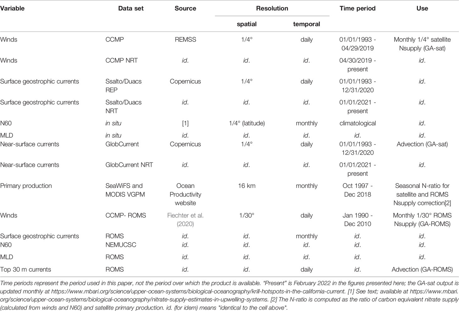
Table 1 List of datasets used as inputs forcing the GA model (GA-sat and GA-ROMS runs described in section Runs and Sensitivity Experiments).

Several of these fields were combined into a monthly, 1/4° resolution coastal nitrate supply product (Nsupply) used to force the GA model. Climatological in situ data sets were also used for nitrate concentration at 60 m depth (N60) and mixed layer depth (MLD). These products were described by Messié et al. (2009) and Messié and Chavez (2015), respectively, although here the MLD criterion was lowered from 0.8°C to 0.2°C (de Boyer Montégut et al., 2004) which, being more sensitive, better captures mixed layer variability in the California Current region. Wind-driven coastal nitrate supply (expressed per meter of coastline) was derived from CCMP wind stress, AVISO surface geostrophic currents, and in situ N60. The method considers both geostrophic and coastal Ekman transports, and was described previously (Messié et al., 2009; Messié and Chavez, 2015; Messié and Chavez, 2017). Coastal upwelling was computed weekly, then positive vertical transports were averaged monthly and multiplied by N60 to estimate coastal nitrate supply. Monthly nitrate supply was corrected for unused nitrate using a seasonal N-ratio (ratio of potential new production and primary production), computed from nitrate supply and satellite primary production over the 1997-2018 time period (see Messié and Chavez, 2015; Messié and Chavez, 2017 for details). Finally, nitrate supply (expressed per m of coast) was converted into a flux per unit volume (hereafter Nsupply, in units of mmolC m^-3 d^-1) by dividing vertically by the seasonal MLD and horizontally by an offshore distance set as the distance between shore and the first wind grid cell (Messié and Chavez, 2017) or 15 km, whichever was higher. Using the first wind grid cell is appropriate for satellite winds but gives unrealistic values for high-resolution ROMS winds available close to shore. The 15-km minimum distance was chosen such that nitrate supply remains consistent when computed from different wind products (QuikSCAT in Messié and Chavez, 2017; 1/4° CCMP and 3 km ROMS post-assimilation winds here), and is similar to the width over which coastal upwelling occurs in ROMS (Jacox et al., 2014, their Figure 1). The CCMP monthly nitrate supply estimates are available at https://www.mbari.org/science/upper-ocean-systems/biological-oceanography/nitrate-supply-estimates-in-upwelling-systems.

ROMS-NEMUCSC

A historical simulation using a coupled physical-biogeochemical model for the central California Current Ecosystem at 1/30° (~3 km) horizontal resolution (Fiechter et al., 2020) was used to evaluate krill distributions predicted by the GA model. The physical component is an implementation of the Regional Ocean Modeling System (ROMS) (Haidvogel et al., 2008) and the biogeochemical component, called NEMUCSC, is a customized version of the North Pacific Ecosystem Model for Understanding Regional Oceanography (NEMURO) model (Kishi et al., 2007) specifically parameterized for the California Current Ecosystem (Fiechter et al., 2018; Fiechter et al., 2020). NEMUCSC includes three limiting macronutrients, two phytoplankton (nanophytoplankton and diatoms), and three zooplankton (micro, meso, and predatory) functional groups. The predatory zooplankton group was parameterized to represent Euphausia pacifica, the numerically dominant euphausiid in the region. The historical ROMS-NEMUCSC solution demonstrated substantial skill in reproducing observed krill hotspots and identified strong patterns of alongshore and seasonal variability in the intensity of these hotspots (Fiechter et al., 2020).

In Situ Surveys

The Rockfish Recruitment Ecosystem Assessment Survey (RREAS) monitors epipelagic micronekton using a mid-water trawl (towed for 15 minutes targeting a 30 m headrope depth at nightime), acoustic surveys to monitor krill distribution and abundance, and visual surveys to map distribution and abundance of seabirds and marine mammals, during late April-June throughout the coast of California (Sakuma et al., 2016; Santora et al., 2021). Acoustic surveys of krill hotspots are summarized by Santora et al. (2018) and visual surveys of top predators are described by Santora et al. (2020) and Santora et al. (2021). Briefly, daytime acoustic and visual surveys are conducted in between hydrographic sampling stations and are standardized by survey effort. For model evaluation purposes, we focused on several applications of this ecosystem monitoring dataset to assess general performance of the GA model in terms of spatial and temporal dynamics involving krill and their predators (Santora et al., 2013; Santora et al., 2017; Fiechter et al., 2020). First, we used the long-term time series of total krill abundance from a subset of consistently sampled 34 stations within the Greater Gulf of the Farallones and Monterey Bay (between 36.6-38.2°N) in late spring (May-June, 1990 to 2019). Standardized mid-water trawls allow for relative total krill abundance estimates based on catch-per-unit-effort (CPUE). Second, for hotspot locations, acoustic measures of the spatial maximum krill abundance (Nautical Area Scattering Coefficient, per 25 km², 2000 to 2015) were compared to model predictions to assess location and occurrence of hotspots (Santora et al., 2011; Santora et al., 2018; Fiechter et al., 2020). Due to the nature of krill aggregation intensity, acoustics are preferred for identifying the location, scale and sizing of krill hotspots, and maximum NASC values are a better representation of hotspots than the mean NASC values. Third, to extend our assessment of observed and modeled krill hotspots to upper trophic levels, we assessed the overall similarity of humpback whale sightings and modeled krill hotspots as a function of latitude (Santora et al., 2017; Cimino et al., 2020; Fiechter et al., 2020; Santora et al., 2020). Counts of humpback whales and model estimates of krill were both binned into 1/4° latitudinal bins and whale sightings were smoothed using a Gaussian weighted 3-point moving average.

Growth-Advection Method

The GA method was developed to simulate zooplankton hotspots in all upwelling systems on a climatological basis (Messié and Chavez, 2017). The method considers the evolution of plankton communities within the surface mixed layer of a water mass advected by near-surface currents, following an input of nutrients by a given process (here coastal upwelling, Figure 1). This is conceptually similar to the idealized mixed-layer conveyor model (Botsford et al., 2003; Botsford et al., 2006), the main difference being that the conveyor model only considered cross-shore displacements while here near-surface currents are used to advect and displace water masses in two dimensions. The GA method was further adapted to include time-varying conditions and applied to island mass effects using a different plankton model initialized by island-driven fertilization (Messié et al., 2020). Here, we combine the plankton model and upwelling initiation process from Messié and Chavez (2017) with the time-varying GA method from Messié et al. (2020) to model zooplankton hotspots off California during the 1993-present time period.

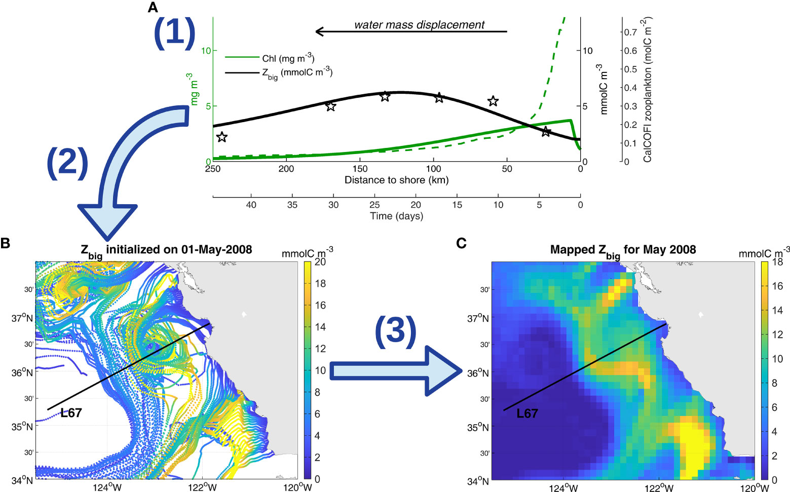
Figure 1 Growth-advection method schematic. (A) Example of NPZ model output (step 1), initialized using the mean nitrate supply off Monterey Bay at 36.8°N (11 mmolC m^-3 d^-1). Z_big (black line) and chlorophyll (green line) outputs are given as a function of time and distance to shore, the correspondence being obtained using a mean offshore speed of 5.6 km d^-1 as in Messié and Chavez (2017). The result is compared to data collected along L67: CalCOFI meso- and macrozooplankton (black stars, see Messié and Chavez, 2017) and MODIS satellite chlorophyll (dashed green line, averaged within 5 km of L67). (B) Example of a daily run (initialized on May 1st, 2008) where the NPZ model is initialized at each latitude using the local CCMP wind-driven nitrate supply (step 1), and Z_big output is mapped onto corresponding 60-day Lagrangian GlobCurrent trajectories initialized at the coast for that latitude (step 2). (C) Example of a monthly map (May 2008) obtained by combining all daily runs into daily maps, further averaged monthly (step 3). The map for May 2008 encompasses runs starting from March 2nd to May 31st, extracting the parts of the trajectories belonging to May.

Specifically, large zooplankton biomass (Z_big) was simulated over time using a simple nutrient, phytoplankton, zooplankton (NPZ) model initialized by Nsupply (GA step 1, Figure 1A). The NPZ model includes new and regenerated nutrients, 2 phytoplankton functional groups, and 2 zooplankton functional groups and was described by Messié and Chavez (2017). This model is slightly simpler than NEMUCSC as it does not include silicate nor detritus, and only includes 2 zooplankton functional groups instead of 3. Z_big was previously parameterized based on copepods (Messié and Chavez, 2017); here all Z_big-related parameters (maximum grazing rate, mortality rate, and excretion rate) were multiplied by 0.6 so that Z_big represents krill (e.g., maximum grazing rate set to 0.36 d^-1 instead of 0.6 d^-1). As a consequence, the Z_big maximum occurs ~ 1 week later and ~ 40 km further offshore relative to Messié and Chavez (2017) (Figure 1A). These new parameters were chosen to match the temporal evolution of the NEMUCSC predatory zooplankton functional group (parameterized to represent E. pacifica, Fiechter et al., 2020) (Figure 2). The plankton model reproduces the average offshore evolution of surface chlorophyll and meso/macrozooplankton well (Figure 1A), except close to shore where satellite chlorophyll is subject to caution and may be enhanced by small-scale retention not captured in Lagrangian trajectories. In both the NPZ model and NEMUCSC, simulated krill peaks ~ 3 weeks after upwelling (Figure 2).

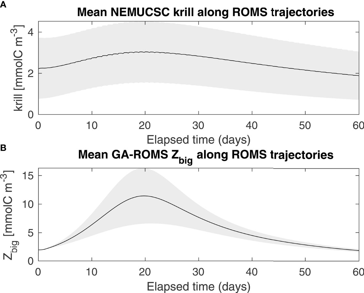
Figure 2 Averaged krill concentration along ROMS trajectories, as represented by NEMUCSC-traj (A) and GA-ROMS (B), originating between 34-44°N between April and August.

The plankton model was initialized using the Nsupply product described above, for a range of dates (daily resolution) and latitudes (3 km resolution) covering the Nsupply spatio-temporal domain. For each day and latitude, plankton concentrations were calculated over time (for 60 days) as a function of Nsupply interpolated in time and latitude. The Z_big output was then mapped onto 60-day near-surface current trajectories originating at the coast at each corresponding 3-km latitude (GA step 2, Figure 1B). The 3-km latitude resolution was chosen to match the ROMS-NEMUCSC model and to ensure sufficient spatial coverage by Lagrangian trajectories. The daily resolution was chosen to better capture temporal variability in horizontal advection rather than in Nsupply (originally monthly). Because of the inherent lag between wind forcing and oceanic response (Service et al., 1998), using a monthly Nsupply reduces the potential mismatch between nutrient delivery and horizontal advection in the model and, thus, produces better estimates of zooplankton distributions compared to using a weekly Nsupply. Current trajectories were computed using the Lagrangian computational tool Ariane (Blanke and Raynaud, 1997). We used a custom version of Ariane specifically designed for surface 2D trajectories (Maes et al., 2018; Messié et al., 2020).

Finally, daily along-trajectory Z_big outputs were combined into 1/8° daily gridded maps by averaging, for each day and each grid cell, all data points from all runs found within this time and space using the Matlab function histcn (Luong, 2011). The daily map grid cells that did not have any coastal trajectory going through were set to 0. Daily maps were further averaged into a monthly product (GA step 3, Figure 1C). The Matlab functions used to run the full GA method are available at https://github.com/messiem/toolbox_GrowthAdvection (doi: 10.5281/zenodo.6494127).

Runs and Sensitivity Experiments

The primary run used in this study, termed GA-sat, was forced using the satellite-based products described above (April 1993-present, 30-46.5°N). While inputs are available starting in January, monthly averages are only calculated when the full Lagrangian temporal coverage is available (i.e., past 60 days). Results until February 2022 are presented here, and GA-sat is updated monthly at https://www.mbari.org/science/upper-ocean-systems/biological-oceanography/krill-hotspots-in-the-california-current. The Nsupply product used to force GA-sat is based on CCMP wind stress, AVISO surface geostrophic currents, climatological in situ N60, climatological in situ MLD, and climatological N-ratio, and is available at https://www.mbari.org/science/upper-ocean-systems/biological-oceanography/nitrate-supply-estimates-in-upwelling-systems. Lagrangian trajectories were computed using GlobCurrent 15-m currents.

A second run, termed GA-ROMS, was computed using forcing from ROMS-NEMUCSC fields (April 1990–December 2010, 32-44°N). The GA-ROMS output was used to assess whether the GA method is able to reproduce results from a fully coupled physical-biogeochemical model (ROMS-NEMUCSC), despite being much simpler and Lagrangian instead of Eulerian. The GA-ROMS forcing fields were derived from ROMS-NEMUCSC outputs and forcing fields so that GA-ROMS and NEMUCSC outputs are directly comparable. The Nsupply product used to force GA-ROMS is based on CCMP-ROMS wind stress after corrections from data assimilation (Neveu et al., 2016), ROMS surface geostrophic currents, monthly NEMUCSC N60, climatological ROMS MLD, and climatological N-ratio computed from satellite primary production over the 1997-2010 time period. Lagrangian trajectories in GA-ROMS were computed using ROMS currents averaged over the top 30m of the water column.

An additional Lagrangian product was derived from the NEMUCSC output by extracting daily NEMUCSC krill along the ROMS Lagrangian trajectories calculated for GA-ROMS. These along-trajectory NEMUCSC krill time series were used to tune the GA model by ensuring that the timing of the offshore maximum predicted by the NPZ model approximately matches that of NEMUCSC (Figure 2). In addition, along-trajectory NEMUCSC krill values were averaged into daily, then monthly, maps following the GA mapping method (GA step 3 in Figure 1). This monthly mapped product, termed NEMUCSC-traj, is useful for two reasons. First, compared to NEMUCSC, NEMUCSC-traj represents krill present only in water masses originating at the coast. Differences between NEMUCSC and NEMUCSC-traj are thus due either to the GA mapping method (GA step 3) or to water masses that did not originate at the coast within the domain (hereafter referred to as “process set #1”). Second, NEMUCSC-traj represents an upper bound for GA-ROMS performance, meaning what GA-ROMS would be if Nsupply and the NPZ model were able to perfectly reproduce the NEMUCSC along-trajectory krill output. Differences between GA-ROMS and NEMUCSC-traj are thus due to differences in the NPZ model formulation relative to the NEMUCSC formulation, offshore nutrient supply, or horizontal mixing between trajectories (hereafter referred to as “process set #2”). For instance, the narrower GA zooplankton peak relative to NEMUCSC (Figure 2) is likely due to the lack of horizontal mixing. The percentage of NEMUCSC variance explained by process set #1 for a given hotspot time series was computed as varex₁ = 1-r₁², where r₁ is the correlation coefficient between NEMUCSC and NEMUCSC-traj. The percentage of NEMUCSC variance explained by process set #2 was computed as varex₂ = 1-varex₁-r₂², where r₂ is the correlation coefficient between NEMUCSC and GA-ROMS.

The GA method allows for sensitivity experiments where environmental drivers can be perturbed independently from one another (Messié and Chavez, 2017). This would not be possible with a coupled model such as ROMS-NEMUCSC, where (for instance) a perturbation of the winds (i.e., upwelling) would also impact other variables such as near-surface currents and subsurface nutrient concentrations including N60. Sensitivity studies considered the effect of upwelling, near-surface currents, and source waters (via N60). They were conducted for both GA-ROMS and GA-sat to explore the role of different predictors in shaping the interannual variability of krill hotspots. For these experiments, a given forcing variable was replaced by its climatology (perturbed run), and the perturbed run was compared to its reference run (GA-ROMS or GA-sat). For each predictor and hotspot, the percentage of GA interannual variance explained exclusively by that predictor was computed as 1-r², where r is the correlation coefficient between the hotspot time series in the perturbed vs reference run.

Results

GA Proof-of-Concept: NEMUCSC “Twin Experiment”

The GA-ROMS model output was compared to that from NEMUCSC to assess the skill of the Lagrangian GA method in representing krill hotspots computed from an Eulerian physical-biogeochemical model. Overall, both spatial and temporal patterns are well represented by GA-ROMS (Figures 3, 4). Modeled biomass is substantially higher for GA, which is not surprising since NEMUCSC includes 3 zooplankton functional groups while GA only represents 2. This is not a significant issue as our goal is to represent krill spatio-temporal variability, such as hotspot location and timing, rather than actual biomass. Both GA-ROMS and NEMUCSC display three major hotspots (areas of elevated krill concentration): one north of Point Conception, one off Monterey and San Francisco Bays, and one between Cape Blanco and Cape Mendocino (Figure 3, hereafter southern, central, and northern hotspots). The location of these hotspots is variable from year to year and as such, a formal definition of hotspot location is challenging. In the following, hotspot boundaries were defined based on coastline features, such as capes, that have been shown to impact biological activity (Fiechter et al., 2018): northern 40.4-42.8°N, central 36.3-38.9°N, and southern 34.5-36°N (Figure 3). The krill patterns produced by GA-ROMS indicate that the GA model correctly reproduces hotspot locations (Figures 3A vs B), seasonal cycle and northward intensity shift (Figure 3C vs D), and interannual variability (Figure 4) identified in the ROMS-NEMUCSC simulation and reported by Fiechter et al. (2020). In particular, GA was able to capture close to 90% of the central and southern hotspot interannual variability. A smaller hotspot is also visible near 40°N in NEMUCSC (discussed by Fiechter et al., 2020), and is underestimated in GA-ROMS. However, interannual variability in the region is correctly represented (r² = 0.57 between Pt Arena and Cape Mendocino, not shown).

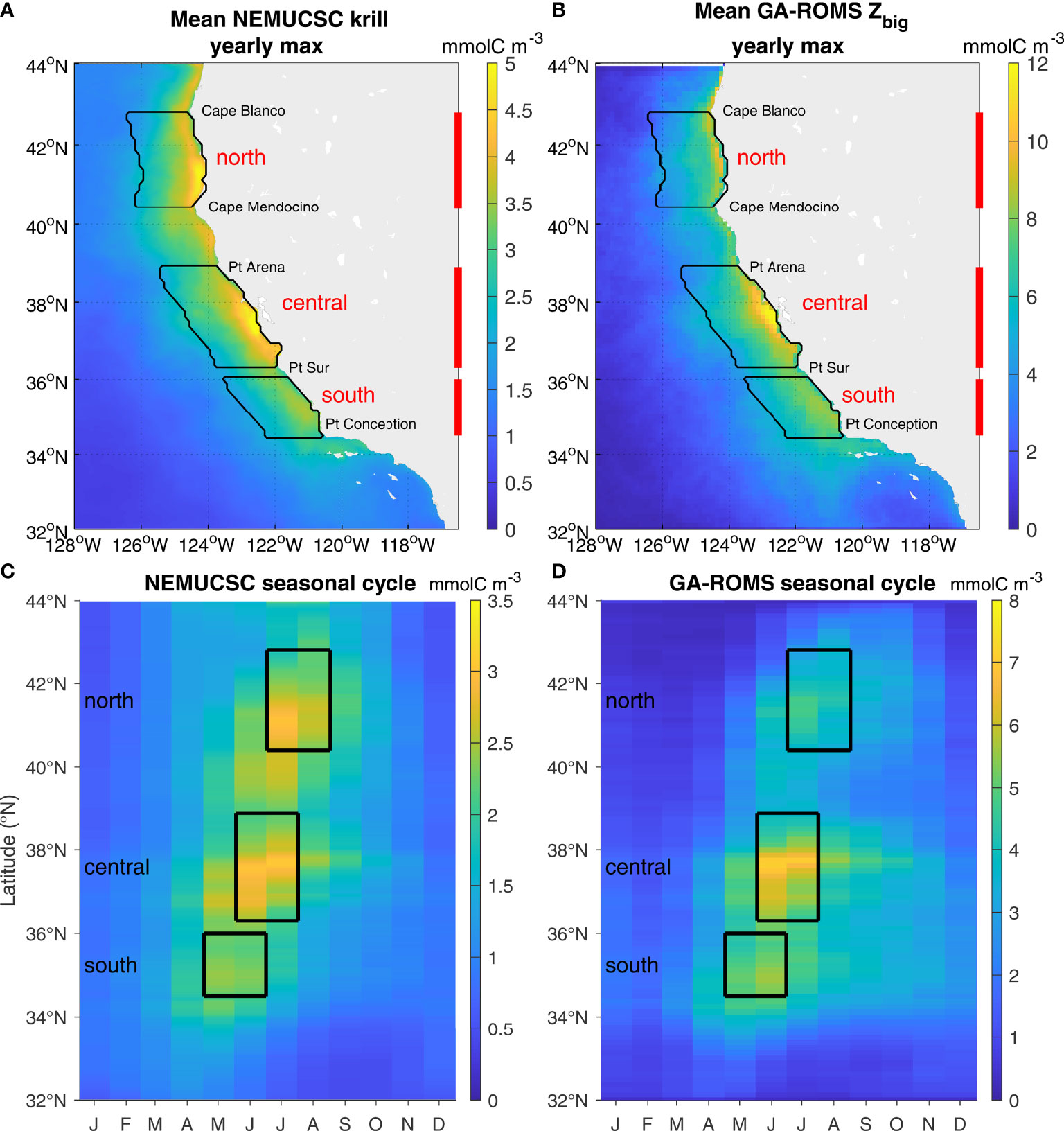
Figure 3 Seasonal distribution of krill hotspots in NEMUCSC and GA-ROMS. (A, B) Spatial patterns: maximum yearly values computed at each grid cell each year, and averaged over all years (1990-2010 time period) for NEMUCSC (A) and GA-ROMS (B). The three main hotspots are contoured in black (north 40.4-42.8°N between Cape Mendocino and Cape Blanco, central 36.3-38.9°N between Point Sur and Point Arena, south 34.5-36°N between Point Conception and Lopez Point, up to 150 km offshore). (C, D) Monthly climatological values averaged within the 150 km coastal band for NEMUCSC (C) and GA-ROMS (D). Black boxes indicate the latitudinal range and peak months of hotspots used to compute the time series presented in Figure 4.

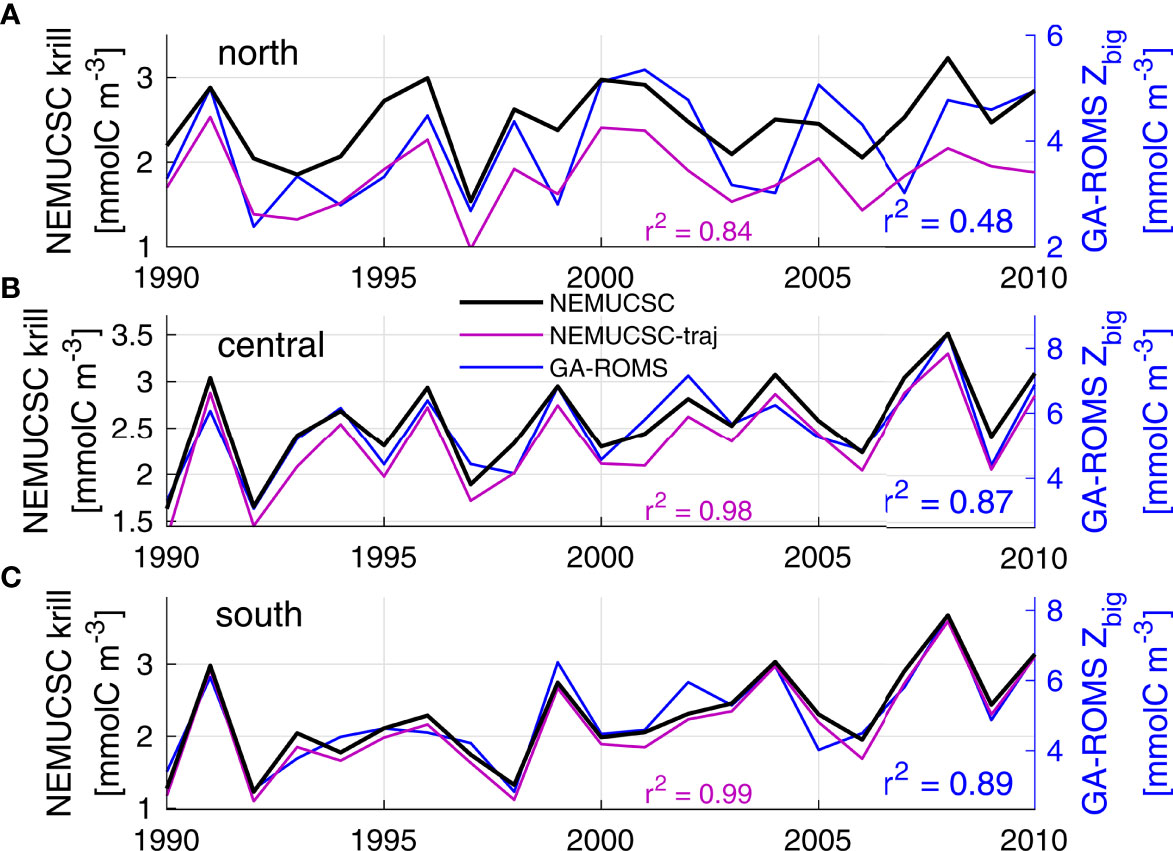
Figure 4 Validation of GA-ROMS interannual variability against NEMUCSC. Panels display yearly time series for each hotspot for NEMUCSC (black), NEMUCSC-traj (purple, same y-axis) and GA-ROMS (blue), obtained by averaging the hotspot region for the peak months each year (see Figure 3): (A) north 40.4-42.8°N July-August, (B) central 36.3-38.9°N June-July, (C) south 34.5-36°N May-June, all up to 150 km offshore. Correlations against NEMUCSC are given for NEMUCSC-traj (purple) and GA-ROMS (blue).

The northern hotspot is less well represented; relative to other hotspots, it is much weaker in GA-ROMS than NEMUCSC (Figure 3) and only 48% of its interannual variability was captured (Figure 4A). The primary reason can be identified by looking at NEMUCSC-traj (Figure 4, purple). Indeed, NEMUCSC-traj almost perfectly represents NEMUCSC for the central and southern hotspot, thereby justifying the use of a Lagrangian method that only considers water masses originating at the coast, and validating the GA mapping method. In contrast, the NEMUCSC-traj krill values are considerably lower than those from NEMUCSC for the northern hotspot, and NEMUCSC-traj represents a lower percentage of NEMUCSC interannual variance than for the central and southern hotspots. This suggests that in NEMUCSC, the northern hotspot is partly driven by water masses that did not originate at the coast. This is not surprising considering how close the northern hotspot is to the ROMS domain boundary at 44°N (Figure 3A); water masses flowing southward through the northern boundary likely contribute to the hotspot (see also section Hotspot Water Mass Origin) and are not represented in NEMUCSC-traj nor by the GA method (no boundary forcing). This is not an issue at the southern boundary since currents are predominantly southward, nor in GA-sat where the latitudinal domain extends to 48°N.

GA-sat Output Evaluation Against In Situ Data

Evaluation of krill spatio-temporal patterns predicted by GA-sat was made with ecosystem survey data spanning multiple decades, but that are restricted seasonally and regionally. GA-sat springtime spatial and temporal patterns are consistent with in situ data (Figures 5, 6). Similar to GA-ROMS and NEMUCSC, GA-sat displays two springtime hotspots also visible in in situ data (Figure 5): a southern hotspot near 35°N (most visible in acoustic sampling) and a central hotspot near 37°N (most visible in trawl sampling). These hotspots are located slightly further offshore in GA-sat relative to in situ data and to NEMUCSC/GA-ROMS, but their alongshore location is correctly represented.

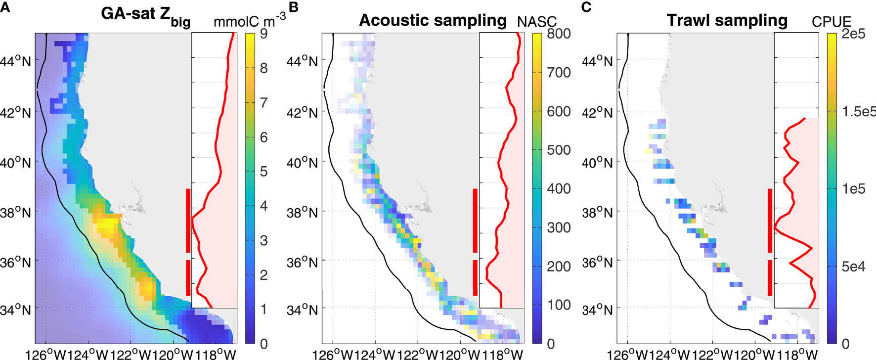
Figure 5 GA-sat krill springtime spatial pattern evaluation against in situ surveys. All panels are May/June averages, and display as an insert the latitudinal profile averaged in the 150 km coastal band (black contour). Red bars indicate the central and southern hotspots (northern hotspots occur later in the year). (A) GA-sat restricted to non-NRT years; pixel transparency indicates the region sampled in situ. (B) Acoustic and (C) trawl in situ data averaged onto the GA-sat grid (data restricted to 2004-2019 when surveys expanded beyond the central region); pixel transparency is inversely proportional to the number of years sampled at each grid cell.

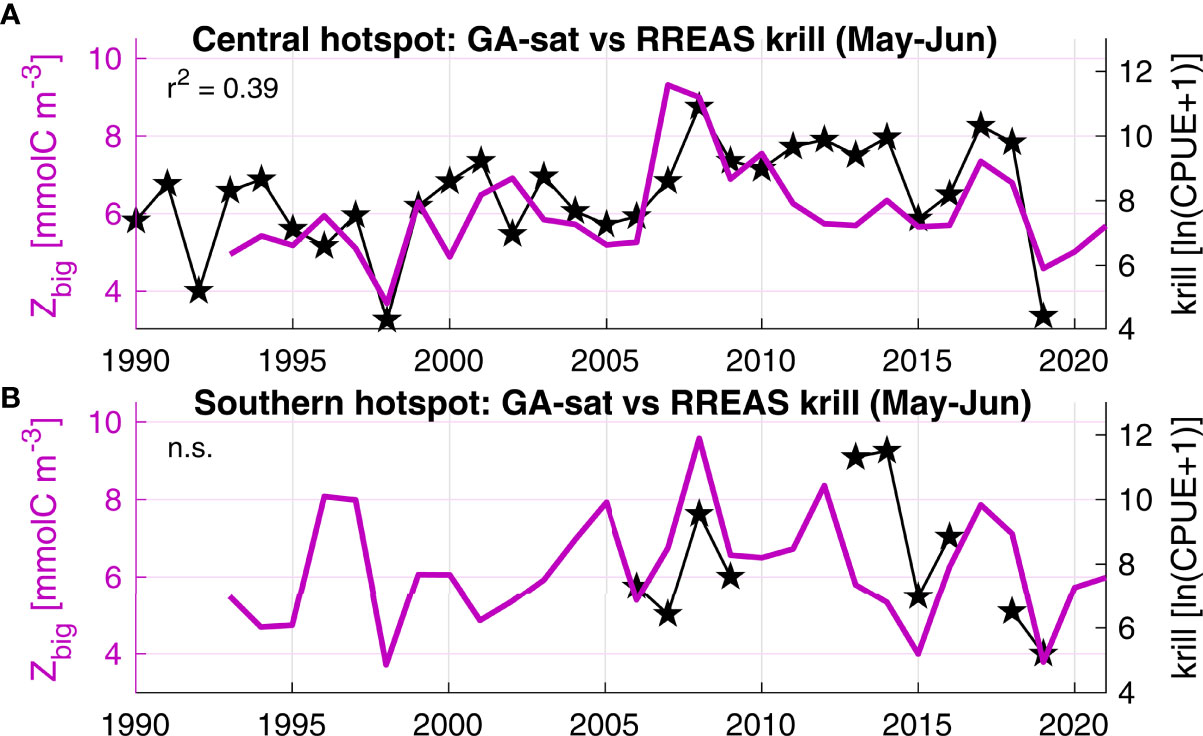
Figure 6 GA-sat temporal variability (purple) evaluated with RREAS trawl krill survey (black). (A) The central hotspot overlaps with the RREAS core area continuously sampled since 1990. Both datasets were averaged during May-June, up to 150 km offshore for GA-sat Z_big. (B) The RREAS also surveys the southern hotspot, although more recently and with less coverage (years with less than 10 trawl stations were excluded). In this region GA-sat Z_big was averaged up to 100 km offshore (the southern hotspot is closer to shore than the central hotspot in GA-sat). The correlation between krill and Z_big is non-significant (n. s.) for the southern hotspot, partly due to the low number of data points.

The time series of modeled and in situ krill data are significantly correlated for the central hotspot (most extensively surveyed, Figure 6A). Broad patterns are correctly represented, including the central hotspot springtime increasing trend identified by Fiechter et al. (2020) over the 1990-2010 time period (and shown here to extend until at least 2018) and the 1998 and 2019 very low krill concentrations. Correlations are non-significant for the southern hotspot for which in situ spatial (Figure 5C) and temporal (Figure 6B) coverage is lower. It is worth noting that the GA and in situ time series remain very similar except in 2013-14, two years that were also underestimated by GA for the central hotspot. Unfortunately, limited survey data is available to evaluate hotspots north of 40°N which are predicted to peak in July-August after the survey (Figure 7).

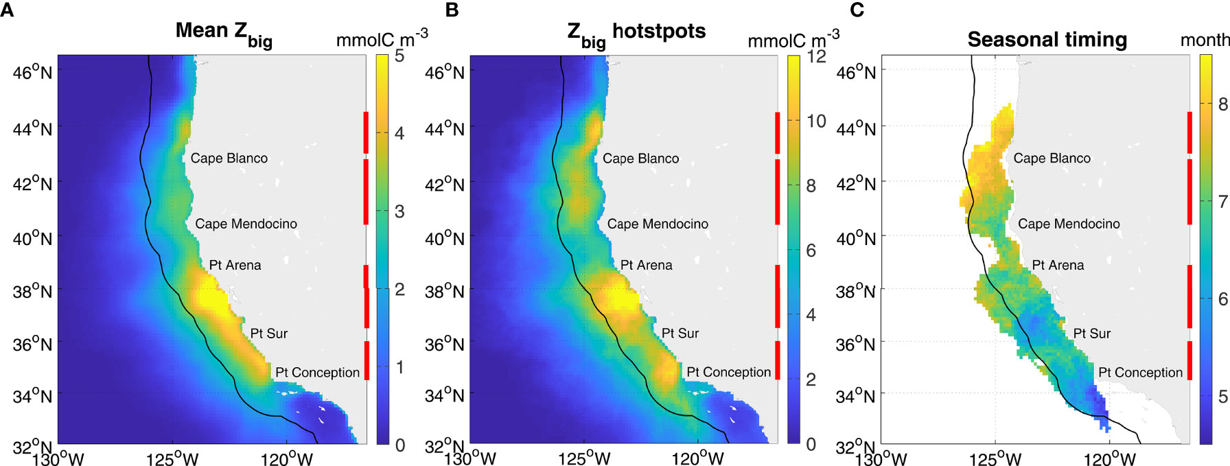
Figure 7 Krill hotspots spatial distribution and timing in GA-sat (1993-2018). The maps display: (A) the mean Z_big, (B) the mean yearly maximum Z_big, and (C) the mean timing of the yearly maximum. For B, C values were computed at each grid cell each year, and averaged over all years. Only grid cells where the mean yearly maximum is over its 80th percentile were retained for seasonal timing. The black contour indicates the 150 km coastal band, and the red bars indicate zooplankton hotspots: northernmost 43-44.5°N, north 40.4-42.8°N, central 36.3-38.9°N, and south 34.5-36°N.

Krill Spatio-Temporal Patterns in the California Current

As a mechanistic model and given its extended spatio-temporal coverage relative to in situ data and to NEMUCSC, GA-sat provides a useful framework to gain new insights on krill broad spatial patterns and temporal variability in the California Current. GA-sat Z_big maps computed over the 1993-2018 time period (excluding NRT forcing fields) indicate that on average, krill concentrations are highest between Point Conception (34.4°N) and Point Arena (38.9°N) (Figure 7). Spatial and seasonal patterns in GA-sat are very similar to features described previously (Figure 3; Fiechter et al., 2020), including the seasonal northern propagation of hotspots, with the caveat that GA-sat hotspots are located slightly too far offshore. In addition to the 3 major hotspots identified previously (Figures 3, 5; Fiechter et al., 2020), a small new hotspot is revealed by GA-sat just north of Cape Blanco near 44°N (hereafter northernmost hotspot), peaking in August. This hotspot is located in a retentive area over a submarine shelf bank (Heceta Bank) where high zooplankton biomass including krill was previously measured in late summer (Ressler et al., 2005; Keister et al., 2009).

The main value of the GA-sat run arguably resides in its representation of krill temporal variability, available from 1993 to present. The GA-sat output represents a 29-year retrospective analysis of krill hotspots in the California Current and indicates strong interannual variability in the strength and location of hotspots (Figure 8). While the central hotspot appears to remain fairly consistent (i.e., visible most years), the other hotspots are more intermittent. Some broad patterns are identifiable at the interannual to decadal time scales including high concentrations from 2007-2013 and overall lower concentrations south of 40°N in 2014-16 during an unusually strong marine heatwave (Di Lorenzo and Mantua, 2016). These patterns are also visible in the May-June RREAS survey (Figure 6). Northern hotspots appear to be particularly intense when the central and southern hotspots are weaker (e.g., 2006, 2014-16), consistent with the second mode of variability in NEMUCSC (Fiechter et al., 2020).

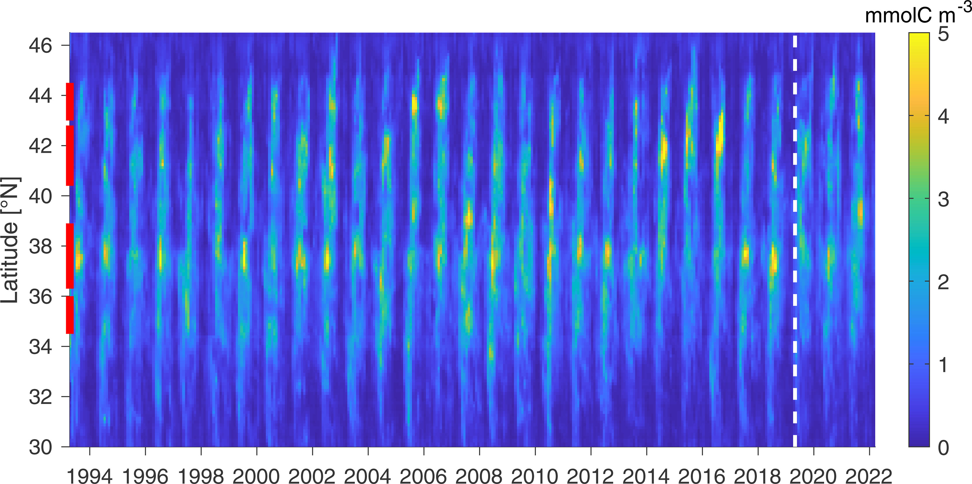
Figure 8 Krill temporal variability: Z_big averaged in a 150 km coastal band (GA-sat, monthly 1/8° resolution). The white dashed line indicates when Z_big became based on NRT satellite products.

In addition, Z_big exhibits significant trends over 1993-2018 (Figure 9). Trends appear strongest in May-June across the domain, while other months see a decrease in Z_big concentrations (e.g., September). Sensitivity experiments using climatological Nsupply or advection indicate that upwelling is the primary driver of spring/summer increases, while advection may be responsible for the fall decrease (not shown). As a consequence of these patterns, stronger trends present during May-June for both Z_big and RREAS krill (Figure 6) are not representative of overall trends. The May-June increasing trend may indicate a shift in the krill seasonal cycle rather than an overall increase in krill concentration (Figure 9A), although overall trends over the entire year remain positive north of 35°N (Figure 9B). The strongest trends are observed near the northern limit of each hotspot, suggesting a northward displacement of each hotspot. The northern hotspot is the only one where peak intensity increased (i.e., positive trend during the hotspot peak, Figure 9A). Trends are slightly stronger in the northern part of the domain, despite being stronger in the southern part during the pre-2010 time period (Fiechter et al., 2020; Figure 8). As a consequence, there is an overall northward displacement of Z_big concentrations across hotspots over the full time period, with northern hotspots increasing faster than southern ones. In summary, Z_big seasonal trends suggest krill hotspots have been shifting northward and occurring progressively earlier in the year. Whether these changes are part of natural low frequency variability or a manifestation of long-term change cannot be determined.

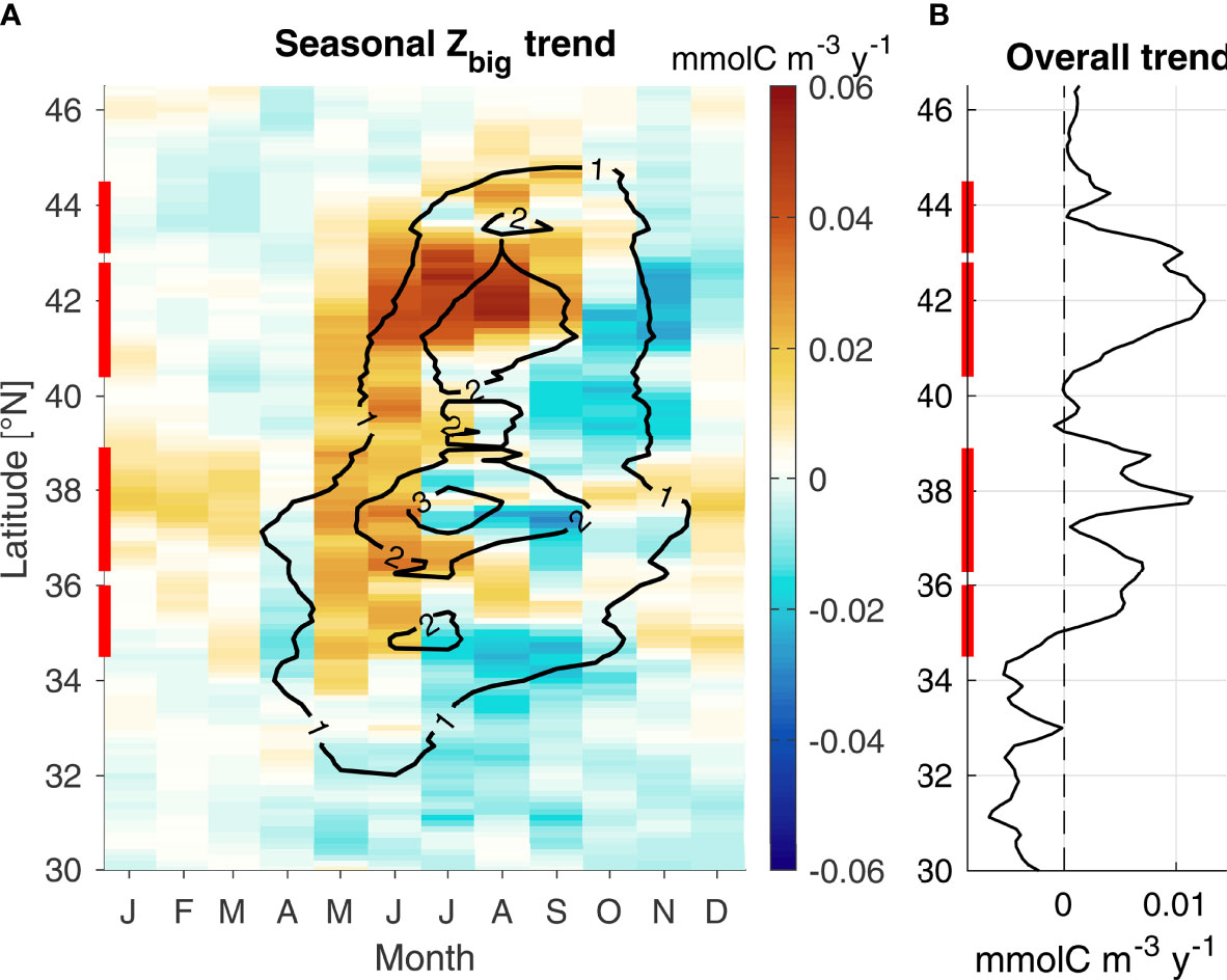
Figure 9 GA-sat Z_big trend (1993-2018). (A) Trend as a function of latitude and month of the year (colors); black contours display the Z_big seasonal cycle (mmolC m^-3). (B) Overall trend calculated at each latitude. Red bars indicate the hotspot locations.

Hotspot Interannual Drivers

Sensitivity studies were conducted for both GA-ROMS and GA-sat using runs where one forcing variable (upwelling, currents, or N60) was replaced by its climatology (see Materials and Methods). Comparing the hotspot yearly variability in the perturbed run versus its reference run (GA-sat or GA-ROMS) reveals how much each forcing variable controls the interannual variability of each hotspot (Table 2). Comparisons for the ROMS forcing runs (left column) provide the most complete picture, because of the availability of the NEMUCSC and NEMUCSC-traj products, and of N60 forcing (the reference GA-sat run is already forced by climatological N60). Comparing hotspot time series in NEMUCSC, NEMUCSC-traj, and GA-ROMS provides information on the impact of non-coastal water masses, the GA mapping method, the use of a simpler time-only plankton model relative to NEMUCSC, and processes represented in ROMS-NEMUCSC that are not represented in GA such as offshore nutrient supply and horizontal/vertical mixing.

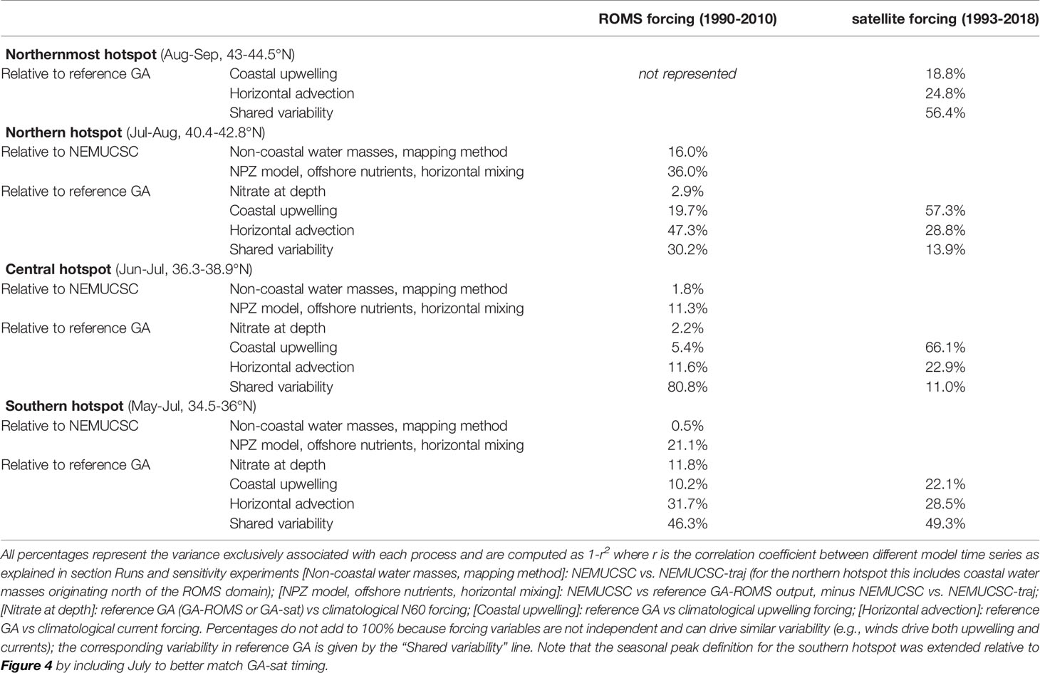
Table 2 Percentage of variance explained by various processes for each yearly hotspot time series.

Comparing NEMUCSC and NEMUCSC-traj confirms that Lagrangian trajectories originating at the coast are sufficient to reproduce most of the hotspots’ interannual variability, except for the northern hotspot where coastal water masses originating north of 44°N are not accounted for. This indicates that hotspot water masses are primarily of coastal origin. Other processes not included in the GA method are responsible for a larger proportion of the variance, including NEMUCSC processes not included in the simpler NPZ model (e.g., detritus), horizontal mixing between Lagrangian trajectories, and along-trajectory offshore nutrient sources (e.g., Ekman pumping or vertical mixing). Overall, processes not represented in the GA method are responsible for 13.1% of the central hotspot and 21.6% of the southern hotspot interannual variability when using ROMS forcing.

Regarding GA drivers (upwelling, advection, and N60), the GA-ROMS sensitivity runs indicate that nitrate at depth plays a minor role in hotspot interannual variability for the central and northern hotspot (< 3%, Table 2). The impact is larger for the southern hotspot but remains relatively small (11.8%). Advection was found to drive hotspot variability more than upwelling for all hotspots in GA-ROMS, while in GA-sat upwelling strongly dominated the central and northern hotspot variability. Despite these differences, some results are consistent between GA-sat and GA-ROMS. First, horizontal advection is identified as a strong driver of hotspot interannual variability: its impact is around 20-30% for all hotspots in GA-sat. Second, the impact of horizontal advection relative to upwelling (e.g., ratio of the two) appears to be strongest for the southern hotspot (and northernmost, not represented in GA-ROMS).

Hotspot Water Mass Origin

The impact of advection on hotspot location was investigated by analyzing Lagrangian trajectories initialized from April to August, which includes all trajectories that contribute to the peak hotspot time period. Trajectories were simplified by only analyzing their origin and destination, defined here as the location where Z_big peaks (Z_peak, observed after ~ 3 weeks, Figure 2B). The latitudinal distribution of trajectory destination for high Z_peak trajectories reproduces the four previously identified hotspots (Figure 10A, yellow and green). When considering all trajectories (dark blue), the figure highlights where trajectories converge or diverge (i.e., latitudes where, respectively, more or less Z_peak locations were found than the number of initialized trajectories). The four major hotspots are observed in convergence regions, although not all convergence regions lead to a hotspot. For instance, convergence regions are visible near 45°N and south of 34°N, but their trajectories were characterized by low Z_peak values and are thus not hotspot regions. In summary, the latitudinal distribution of hotspots predicted by the GA model is driven by current convergence and divergence, along with coastal nitrate supply.

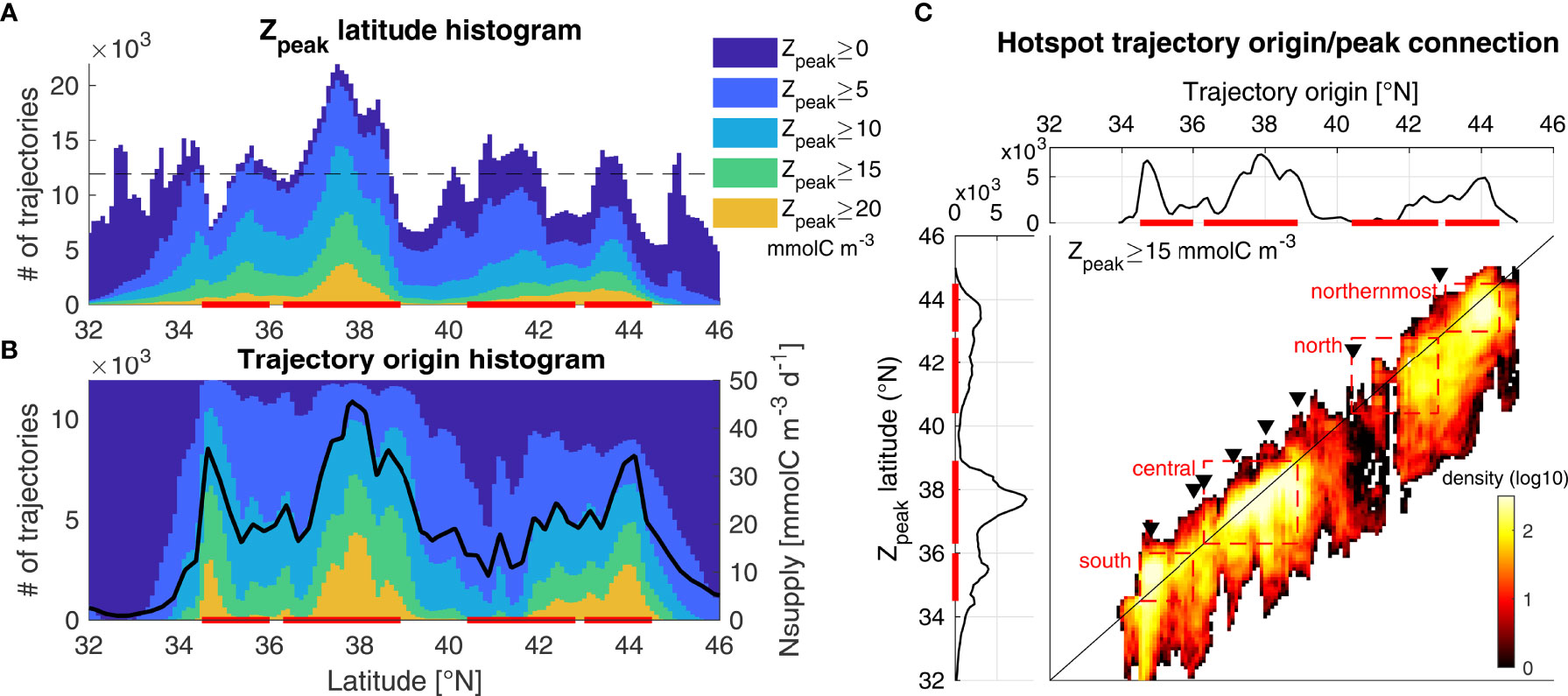
Figure 10 Origin of krill hotspots. The figure connects, for each trajectory initialized from April to August, the latitudes of its coastal origin and its Z_big peak (Z_peak, observed after ~ 3 weeks). (A) Histogram of Z_peak latitudes, where dark blue encompasses all trajectories and successive colors restrict trajectories to those where Z_peak is above a given threshold. The dashed line represents the number of trajectories initialized at each latitude bin, meaning that waters converge wherever the dark blue histogram (all trajectories) is above and diverge where it is below. (B) Corresponding histogram of water mass origin for the same thresholds. The dark blue histogram is flat since the same number of trajectories is initialized in each latitude bin. The dark line represents the mean nitrate supply during April-August. (C) Example of connection between Z_peak and trajectory origin for the 15 mmolC m^-3 threshold (corresponding to the green color in a and b), where the x-axis (and top horizontal panel) is the trajectory origin, the y-axis (and left vertical panel) is the Z_peak latitude, and colors indicate the number of corresponding trajectories. Each row in the density plot displays where hotspot water masses at that latitude originated from, and each column displays where Z_big peaks along water masses originating from that latitude. Black triangles indicate major capes, from south to north: Pt Conception, Lopez Pt, Pt Sur, Pt Ano Nuevo, Pt Reyes, Pt Arena, Cape Mendocino, and Cape Blanco. The strong upwelling near 44°N is not associated with a cape. The Z_peak latitudes were smoothed using a 3-point window in all plots, and histograms were constructed at 1/10° resolution. Red bars highlight the hotspots’ latitude.

While Z_peak is proportional to the initial Nsupply input, high nitrate supply regions do not always coincide with high Z_peak regions (Figure 10B). For example, the Point Conception upwelling center (~ 34.5°N) is characterized by a strong nitrate supply peak (black line) that led to a large number of high Z_peak trajectories originating there (yellow and green colors); however, no peak is evident at that location in the Z_peak histogram (Figure 10A). In general, the distribution of high Z_peak trajectory origins is very similar to the latitudinal nitrate supply profile (Figure 10B), but different from the hotspot distribution (trajectory destination, Figure 10A). In particular, the distribution of high Z_peak trajectory destinations is characterized by broader peaks than the distribution of high Z_peak trajectory origins, indicating that surface currents tend to spread hotspots rather than concentrate them (except for the central hotspot).

The link between trajectory origin and destination can be visualized for one Z_peak category (corresponding to green+yellow colors in Figures 10A, B) in Figure 10C. Most of the trajectory locations (colors) are found below the 1:1 line (black) indicating that the trajectory destination is most often south of the trajectory origin, which is not surprising as near-surface currents are mostly equatorward. As a consequence, most hotspots (y-axis distribution) are located near or to the south of upwelling centers (x-axis distribution). An exception is the Point Conception upwelling center, where trajectory destinations are mostly found north of the 1:1 line, indicating poleward displacement. Water masses originating from Point Conception get displaced both northward and southward, with a large proportion exiting south of the southern hotspot (red box), which can explain why surface advection plays such a strong role driving this hotspot’s temporal variability (Table 2). While trajectory origin and destination are spatially separated, the separation is small enough that most trajectories remain within the same hotspot region they originated from (Figure 10C red boxes and Table 3). This indicates that hotspot regions account for the majority of their own hotspot production and that there is relatively little water mass exchange between hotspots at the time scales investigated here (~ 3 weeks between upwelling and Z_peak). An exception is the northern hotspot, for which almost half of water masses originate from further north, largely from the northernmost hotspot. This supports the assumption that the poor representation of the northern hotspot in GA-ROMS was due to the 44°N ROMS boundary. This also suggests that the northern and northernmost hotspots may be considered as one with variable location (see also Figure 8A: rarely are 2 separate hotspots visible north of 40°N). The southern hotspot also has a significant contribution from the central hotspot, but not as large (22%).

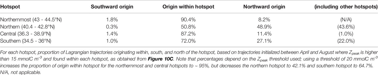
Table 3 Hotspot origin statistics.

Discussion

GA Skills and Implications for Hotspot Drivers

The GA skills in reproducing krill spatio-temporal patterns were assessed using GA-ROMS as a proof of concept (evaluated against NEMUCSC) and GA-sat comparisons against in situ krill surveys. The level of agreement between GA-ROMS and NEMUCSC model simulations indicates that the GA method can simulate krill hotspots that are predicted by a more complex coupled physical-biogeochemical model (except for the northern hotspot near the model boundary), including close to 90% of their interannual variance (Figure 4). This is remarkable considering that the GA method only considers upwelling and advection processes acting on a plankton model itself solely based on temporal dynamics. These results lend confidence that GA-sat can be used to represent krill hotspots, and justifies some of the choices made (or indicates that these have little impact on results) such as the nitrate supply calculation using a fixed 60 m depth for upwelled water mass origin and the use of a time-dependent simpler NPZ model. In addition, the GA skills relative to NEMUCSC indicate that processes not included in the GA method, such as horizontal and vertical mixing and offshore nutrient supply, are of lesser importance.

GA-ROMS sensitivity experiments also suggest that N60 is not a strong driver of interannual hotspot variability, which was unexpected because winter pre-conditioning has been shown to impact the California Current food chain (Schroeder et al., 2013) including krill (Cimino et al., 2020). In the GA model, N60 is the only forcing variable that would be impacted by winter conditions as stronger winter upwelling would result in higher nitrate concentration at depth. Our results suggest that either N60 is not strongly impacted by winter upwelling in ROMS (but rather by contemporary upwelling or source waters), or that winter conditions are a minor contributor to krill variability relative to conditions 2-4 weeks before (lag between upwelling and high Z_big in the model, Figure 2). Regardless, this finding also implies that the lack of interannual N60 forcing in GA-sat probably has little impact on model results. The relatively low degree of importance of N60 and the high percentage of shared variability in GA-ROMS (Table 2) likely mean that upwelling and N60 have similar effects on krill in the California Current (increase or decrease). This may not be the case in other upwelling systems, particularly off Peru where coastal upwelling winds intensify during El Niño while N60 decreases dramatically (Barber and Chavez, 1983).

Comparisons of GA-sat simulations and in situ krill (Figures 5, 6) indicate that overall, GA-sat succeeds in representing broad springtime krill spatial patterns and temporal variability, and suggests that GA-sat should also correctly reproduce broad krill patterns for other seasons and spatial locations. One exception may be the Channel Islands region, where acoustic data reveal a krill hotspot not well represented by the models (Figure 7B; Santora et al., 2011), perhaps due to some island-specific processes. Moreover, it should be noted that GA only captures krill mesoscale variability, not small-scale distribution and patchiness that are tied to bathymetric features such as submarine canyons (Santora et al., 2018). These would be strongly driven by krill behavior (diel vertical migration and swimming) and small-scale currents, currently unresolved by satellites. The advent of new satellites such as the Surface Water and Ocean Topography (SWOT) satellite (launch date fall 2022) will provide a view of oceanic circulation at high spatial resolution, which could help better characterize the impact of topographically-driven currents on krill concentrations. Nevertheless, even at the mesoscale, near real-time prediction of krill hotspots would greatly benefit ecosystem-based management and potential status and health of krill-dependent species and fisheries.

The GA framework highlights the role of upwelling, oceanic circulation, and plankton temporal dynamics in shaping krill mesoscale distribution, seasonal northward propagation, and interannual variability. Plankton dynamics create a temporal decoupling between upwelling and peak krill biomass of ~ 3 weeks in the model (Figure 2), which matches increased calls and aggregations of blue whales, a krill predator, ~ 2-3 weeks after upwelling events in New Zealand (Barlow et al., 2021). This temporal decoupling translates into a spatial decoupling driven by near-surface currents. Assessing the relative importance of upwelling vs horizontal advection in driving krill hotspots is challenging due to conflicting results between GA-ROMS and GA-sat (Table 2). This discrepancy is partly explained by the higher current resolution in GA-ROMS (3 km) than GA-sat (25 km), resulting in smaller scale circulation features (and hence higher variability) being included in GA-ROMS. Another complicating factor is that upwelling- and advection-driven variability are strongly correlated in GA-ROMS, resulting in small percentages of variance explained (particularly for the central hotspot with percentages below 12%). Regardless, even at the mesoscale, our results highlight ocean circulation as a strong driver of krill spatial and interannual variability. The impact of horizontal advection on hotspot location had been shown previously (Dorman et al., 2015a; Messié and Chavez, 2017; Fiechter et al., 2020), but its impact on temporal variability had not yet been identified to our knowledge. Mathematically in the GA method, advection impacts hotspot temporal variability by controlling the area where high concentrations are observed (i.e., trajectory destination). Oceanic circulation is also tied to habitat compression (via the offshore spreading of cold waters), which may explain why the availability of forage species (krill and anchovy) was better related to the area of thermal upwelling habitat than to upwelling indices (Santora et al., 2020).

GA Method Strengths and Weaknesses

The GA method is a fairly simple model in a Lagrangian framework that exclusively represents upwelling, advection, and biological processes in a 2D (horizontal) setting. This simplicity was deliberate, because the results are then less sensitive to parameterization and arguably easier to interpret. Despite its simplicity, the method succeeds in reproducing results from a more complex coupled physical-biological model and observed in situ krill patterns. The potential loss in performance relative to fully coupled physical-biogeochemical models is offset by several advantages. The model does not require high computing power (i.e., it can be run on a laptop) and the satellite-based model enables near real-time calculations. The GA method also allows for independent manipulation of forcing variables which helps separate and quantify drivers (Table 2). Finally, the Lagrangian framework provides a novel view of water mass pathways as they relate to plankton concentration and hotspot formation (Figure 10).

Despite its success in representing broad krill patterns in the California Current, the model has several caveats that should be kept in mind (see also discussion in Messié and Chavez, 2017). Several important processes are not included in the model, in particular those related to krill life cycle and behavior. Diel vertical migration (DVM) is not represented and including DVM could help retain krill closer to shore (Carr et al., 2008; Dorman et al., 2015a), although impacts on temporal variability are less clear. The lack of “biological memory” can impact temporal variability and could play an important role (see discussion in Dorman et al., 2015b). Here, Z_big only depends on conditions up to 2 months prior, while E. pacifica has a lifespan of ~ 2 years (Shaw et al., 2021). However, in situ krill interannual autocorrelation is even weaker than for Z_big (for time series in Figure 6B: 0.18 for RREAS krill, 0.36 for GA-sat Z_big), suggesting biological memory can be neglected for interannual variations. Despite the lack of DVM and life cycle parameterization, GA-sat very satisfactorily represents in situ krill temporal variability considering krill patchiness and survey resolution. Taken together, these results suggest that biological processes such as DVM and life cycle may be of secondary importance when considering broad krill spatio-temporal patterns.

Ecosystem Considerations

Krill is a key trophic link in the California Current, being important grazers of phytoplankton and the primary food source for small pelagic fish and top predators (Croll et al., 2005; Espinoza et al., 2009; Pikitch et al., 2014). Krill hotspots are critical to the functioning of marine ecosystems because their dense aggregations serve as conduits for trophic transfer in marine food webs (Field et al., 2006). Consequently, krill hotspots often coincide with increased abundance of higher trophic level species (Sigler et al., 2012; Santora et al., 2014; Santora et al., 2017; Fiechter et al., 2020). Recently, Santora et al. (2021) identified a suite of seabirds and mammals belonging to a ‘coastal species assemblage’ whose spatial patterns resemble krill hotspots. The same authors identified high biodiversity areas of top predators that are located within krill hotspot regions. These results are based on mean conditions during the springtime RREAS survey; however, similarities between Z_big and latitudinal distributions of whale for individual surveys (Figure 11) suggest that temporal variability in predator distribution may be tied to krill distribution as represented by GA-sat. Therefore, krill model output can inform studies of krill-predators through providing indices for assessing functional relationships (i.e., predator diet and reproduction), and for monitoring near real time ecosystem shifts related to krill availability that result in changes in predator distribution. For example, recent increases in whale entanglements were related to changes in krill hotspot availability where a decline in krill abundance (hotspot intensity) resulted in a shoreward shift of whales inshore, resulting in increased overlap with commercial fishing gear (Santora et al., 2020). A management challenge of protected species within the California Current is determining resource needs as a function of prey availability to prevent adverse impacts on either recovering or commercially important species. Whale migrations to and from the seasonally productive California Current likely depend on the timing, duration and formation of prey hotspots. Humpback whales migrating north in the spring encounter the southern hotspot first and may defer northward movements depending on the concentration of prey available (or vice versa). This may explain some of the patterns visible in yearly whale distributions (e.g., 2004 to 2006, Figure 11). Therefore, the operational GA satellite model provides predictions that could be a potentially powerful tool for ecosystem assessments and monitoring, as well as making predictions about changes in marine food webs due to both natural and anthropogenic climate change.

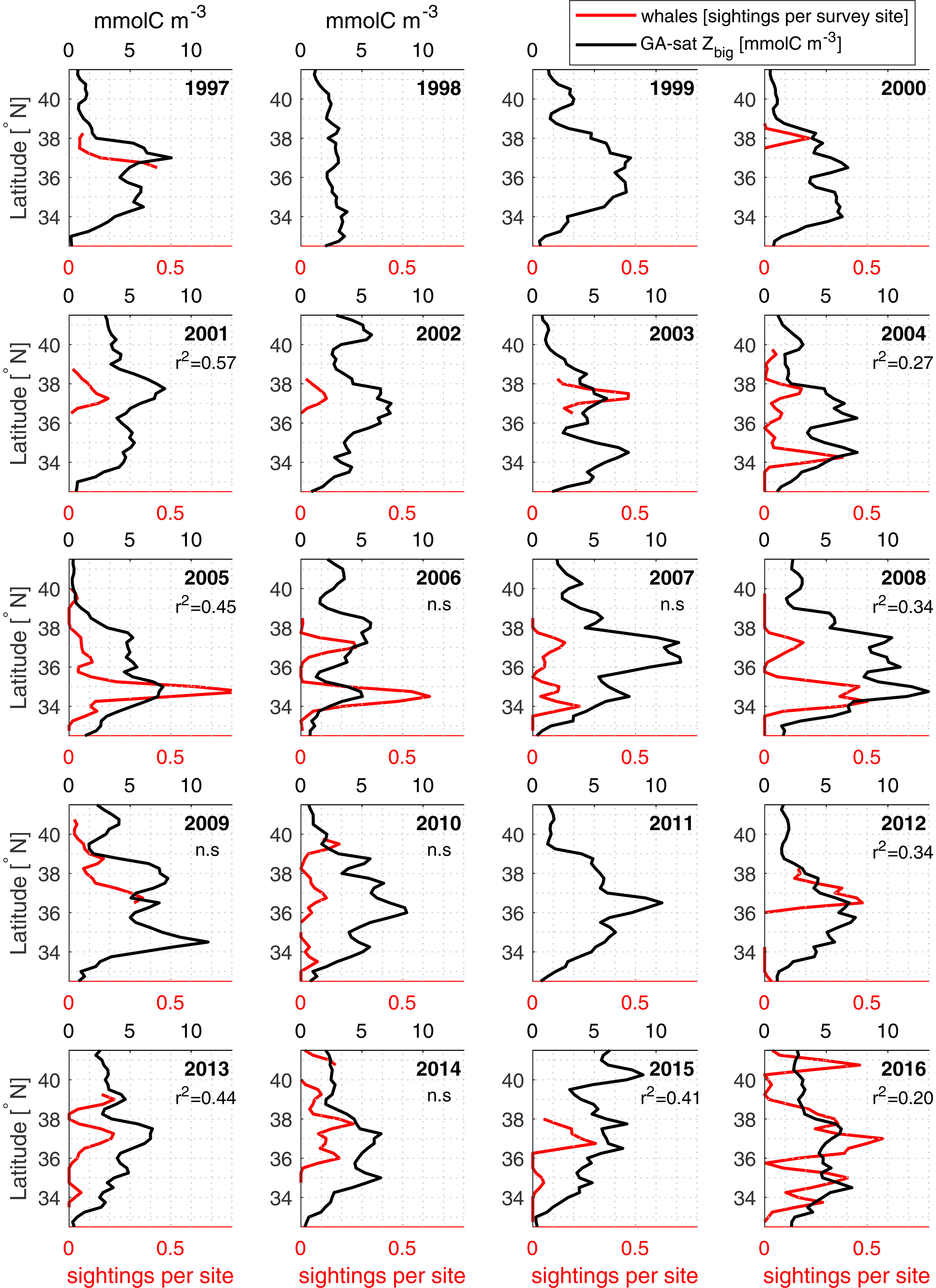
Figure 11 Comparison of GA-sat output and humpback whale sightings. Yearly latitudinal profiles comparing humpback whale sightings from RREAS divided by total sites surveyed (red) against GA-sat Z_big (black). Whale surveys occurred predominantly in May (74% of samples) but also include sightings from late April (9%) and early June (17%). GA-sat Z_big was averaged within 150 km from shore during the month of May. Correlation squared are reported when whale sightings are available over at least 2° latitude; n.s. indicates non-significant correlations (p > 0.05). As explained in text, a direct correspondence is not expected.

Conclusion

This study demonstrates that the GA model, previously shown to be able to reproduce average krill hotspot spatial patterns off California (Messié and Chavez, 2017), can also reproduce krill spatio-temporal variability when using time-varying forcing fields. Interannual variability in the GA-sat output is only driven by satellite-derived upwelling and near-surface oceanic currents, highlighting the importance of both upwelling and horizontal advection in shaping zooplankton spatial and temporal patterns. Connecting hotspots with their coastal origin within the GA Lagrangian framework suggests that two conditions are necessary for a hotspot to form: a convergence of coastal water masses, and above average coastal nutrient supply where these water masses originated from. Our analysis also indicates that zooplankton hotspots are decoupled in time (~ 3 weeks) and space (mostly up to ~ 2° latitude) from upwelling centers (Fiechter et al., 2020). We found that > 70% of water masses originate from within each hotspot (with the exception of the northern hotspot ~ 50%), the rest being of northern origin.

Our results can have significant implications for ecosystem management since krill hotspots (both observed and modeled) coincide with important ecosystem characteristics such as biodiversity and species assemblage (Santora et al., 2021). Whether these relationships hold for temporal variability remains to be demonstrated, but simple comparisons with whale sightings suggest that they may. The GA-sat output is available online and updated monthly (https://www.mbari.org/science/upper-ocean-systems/biological-oceanography/krill-hotspots-in-the-california-current).

Data Availability Statement

The datasets presented in this study can be found in online repositories. The names of the repository/repositories and accession number(s) can be found below: The primary data sets used in this study are available for the 1993-2018 time period (excluding NRT forcing) at https://doi.org/10.5281/zenodo.6415214. They include the GA-sat Zbig model output and the CCMP-based nitrate supply used to force the model. Both are available up to present (using NRT forcing) and uploaded monthly at https://www.mbari.org/science/upper-ocean-systems/biological-oceanography/krill-hotspots-in-the-california-current and https://www.mbari.org/science/upper-ocean-systems/biological-oceanography/nitrate-supply-estimates-in-upwelling-systems, respectively. Data origin for forcing fields is given in section "Materials and Methods". ROMS-NEMUCSC outputs can be accessed at https://doi.org/10.7291/D1KD4J, and RREAS catch data at https://coastwatch.pfeg.noaa.gov/erddap/tabledap/FED_Rockfish_Catch.html.

Author Contributions

MM conceived and designed the study, developed the Growth-Advection model, and led the interpretations and writing. MM and DS-G performed the data analyses. JF provided the ROMS-NEMUCSC outputs and JS provided the RREAS data; both significantly contributed to the paper writing. MM, DS-G, JF, JAS, and FPC contributed to discussions and interpretations that shaped the study and the manuscript. All authors contributed to the article and approved the submitted version.

Funding

This study was primarily funded by a grant from the National Aeronautics and Space Administration (80NSSC17K0574), with additional support by the David and Lucile Packard Foundation and by the US Marine Biodiversity Observation Network jointly funded by NOAA, NASA, and the National Oceanographic Partnership Program (80NSSC20M0001).

Conflict of Interest

The authors declare that the research was conducted in the absence of any commercial or financial relationships that could be construed as a potential conflict of interest.

Publisher’s Note

All claims expressed in this article are solely those of the authors and do not necessarily represent those of their affiliated organizations, or those of the publisher, the editors and the reviewers. Any product that may be evaluated in this article, or claim that may be made by its manufacturer, is not guaranteed or endorsed by the publisher.

Acknowledgments

We thank Devon Northcott for early analyses and discussions that helped shape the results presented here, and Nicolas Grima for his help with Ariane. This study has been conducted using E.U. Copernicus Marine Service Information (GlobCurrent and AVISO geostrophic currents). CCMP Version-2.0 vector wind analyses are produced by Remote Sensing Systems.

Abbreviations

CPUE, Catch Per Unit Effort; GA, Growth-Advection; GA-ROMS, GA model forced using ROMS-NEMUCSC fields; GA-sat, GA model forced using satellite fields; NEMUCSC, custom NEMURO version for the California Current System; NEMUCSC-traj, NEMUCSC krill extracted alongside coastal ROMS trajectories; NEMURO, North Pacific Ecosystem Model for Understanding Regional Oceanography; ROMS, Regional Ocean Modeling System; RREAS, Rockfish Recruitment Ecosystem Assessment Survey; Z_big, large zooplankton simulated by the GA model, representing krill; Z_peak, Z_big peak along current trajectories.

References

Abraham C., Sydeman W. (2006). Prey-Switching by Cassin's Auklet Ptychoramphus Aleuticus Reveals Seasonal Climate-Related Cycles of Euphausia Pacifica and Thysanoessa Spinifera. Mar. Ecol. Prog. Ser. 313, 271–283. doi: 10.3354/meps313271
Ainley D., Spear L., Allen S. (1996). Variation in the Diet of Cassin's Auklet Reveals Spatial, Seasonal, and Decadal Occurrence Patterns of Euphausiids Off California, USA. Mar. Ecol. Prog. Ser. 137, 1–10. doi: 10.3354/meps137001
Atkinson A., Siegel V., Pakhomov E., Rothery P., Loeb V., Ross R., et al. (2008). Oceanic Circumpolar Habitats of Antarctic Krill. Mar. Ecol. Prog. Ser. 362, 1–23. doi: 10.3354/meps07498
Atlas R., Hoffman R. N., Ardizzone J., Leidner S. M., Jusem J. C., Smith D. K., et al. (2011). A Cross-Calibrated, Multiplatform Ocean Surface Wind Velocity Product for Meteorological and Oceanographic Applications. Bull. Am. Meteorol. Soc. 92 (2), 157–174. doi: 10.1175/2010BAMS2946.1
Barber R. T., Chavez F. P. (1983). Biological Consequences of El Niño. Science 222, 1203–1210. doi: 10.1126/science.222.4629.1203
Barlow D. R., Klinck H., Ponirakis D., Garvey C., Torres L. G. (2021). Temporal and Spatial Lags Between Wind, Coastal Upwelling, and Blue Whale Occurrence. Sci. Rep. 11 (1):6915. doi: 10.1038/s41598-021-86403-y
Behrenfeld M. J., Falkowski P. G. (1997). Photosynthetic Rates Derived From Satellite-Based Chlorophyll Concentration. Limnol. Oceanogr. 42 (1), 1–20. doi: 10.4319/lo.1997.42.1.0001
Blanke B., Raynaud S. (1997). Kinematics of the Pacific Equatorial Undercurrent: An Eulerian and Lagrangian Approach From GCM Results. J. Phys. Oceanogr. 27 (6), 1038–1053. doi: 10.1175/1520-0485(1997)027<1038:KOTPEU>2.0.CO;2
Botsford L. W., Lawrence C. A., Dever E. P., Hastings A., Largier J. (2003). Wind Strength and Biological Productivity in Upwelling Systems: An Idealized Study. Fish. Oceanogr. 12 (4-5), 245–259. doi: 10.1046/j.1365-2419.2003.00265.x
Botsford L. W., Lawrence C. A., Dever E. P., Hastings A., Largier J. (2006). Effects of Variable Winds on Biological Productivity on Continental Shelves in Coastal Upwelling Systems. Deep Sea Res. Part II: Topical Stud. Oceanogr. 53 (25-26), 3116–3140. doi: 10.1016/j.dsr2.2006.07.011
Brinton E., Townsend A. (2003). Decadal Variability in Abundances of the Dominant Euphausiid Species in Southern Sectors of the California Current. Deep Sea Res. Part II: Topical Stud. Oceanogr. 50 (14-16), 2449–2472. doi: 10.1016/s0967-0645(03)00126-7
Carr S. D., Capet X. J., McWilliams J. C., Pennington J. T., Chavez F. P. (2008). The Influence of Diel Vertical Migration on Zooplankton Transport and Recruitment in an Upwelling Region: Estimates From a Coupled Behavioral-Physical Model. Fish. Oceanogr. 17 (1), 1–15. doi: 10.1111/j.1365-2419.2007.00447.x
Cimino M. A., Santora J. A., Schroeder I., Sydeman W., Jacox M. G., Hazen E. L., et al. (2020). Essential Krill Species Habitat Resolved by Seasonal Upwelling and Ocean Circulation Models Within the Large Marine Ecosystem of the California Current System. Ecography 43 (10), 1536–1549. doi: 10.1111/ecog.05204
Croll D. A., Marinovic B., Benson S., Chavez F. P., Black N., Ternullo R., et al. (2005). From Wind to Whales: Trophic Links in a Coastal Upwelling System. Mar. Ecol. Prog. Ser. 289, 117–130. doi: 10.3354/meps289117
de Boyer Montégut C., Madec G., Fischer A. S., Lazar A., Ludicone D. (2004). Mixed Layer Depth Over the Global Ocean: An Examination of Profile Data and a Profile-Based Climatology. J. Geophys Res. 109, C12003. doi: 10.1029/2004JC002378
Di Lorenzo E., Mantua N. (2016). Multi-Year Persistence of the 2014/15 North Pacific Marine Heatwave. Nat. Climate Change 6 (11), 1042–1047. doi: 10.1038/nclimate3082
Dorman J. G., Sydeman W. J., Bograd S. J., Powell T. M. (2015b). An Individual-Based Model of the Krill Euphausia Pacifica in the California Current. Prog. Oceanogr. 138, 504–520. doi: 10.1016/j.pocean.2015.02.006
Dorman J. G., Sydeman W. J., Garcia-Reyes M., Zeno R. A., Santora J. A. (2015a). Modeling Krill Aggregations in the Central-Northern California Current. Mar. Ecol. Prog. Ser. 528, 87–99. doi: 10.3354/meps11253
Espinoza P., Bertrand A., van der Lingen C. D., Garrido S., de Mendiola B. R. (2009). Diet of Sardine (Sardinops Sagax) in the Northern Humboldt Current System and Comparison With the Diets of Clupeoids in This and Other Eastern Boundary Upwelling Systems. Prog. Oceanogr. 83 (1-4), 242–250. doi: 10.1016/j.pocean.2009.07.045
Fiechter J., Edwards C. A., Moore A. M. (2018). Wind, Circulation, and Topographic Effects on Alongshore Phytoplankton Variability in the California Current. Geophys Res. Lett. 45 (7), 3238–3245. doi: 10.1002/2017gl076839
Fiechter J., Santora J. A., Chavez F., Northcott D., Messié M. (2020). Krill Hotspot Formation and Phenology in the California Current Ecosystem. Geophys Res. Lett. 47 (13). doi: 10.1029/2020gl088039
Fiedler P. C., Reilly S. B., Hewitt R. P., Demer D., Philbrick V. A., Smith S., et al. (1998). Blue Whale Habitat and Prey in the California Channel Islands. Deep Sea Res. Part II: Topical Stud. Oceanogr. 45 (8-9), 1781–1801. doi: 10.1016/s0967-0645(98)80017-9
Field J., Francis R., Aydin K. (2006). Top-Down Modeling and Bottom-Up Dynamics: Linking a Fisheries-Based Ecosystem Model With Climate Hypotheses in the Northern California Current. Prog. Oceanogr. 68 (2-4), 238–270. doi: 10.1016/j.pocean.2006.02.010
Haidvogel D., Arango H., Budgell W., Cornuelle B., Curchitser E., Lorenzo E. D., et al. (2008). Ocean Forecasting in Terrain-Following Coordinates: Formulation and Skill Assessment of the Regional Ocean Modeling System. J. Comput. Phys. 227 (7), 3595–3624. doi: 10.1016/j.jcp.2007.06.016
Harvey C. J., Fisher J. L., Samhouri J. F., Williams G. D., Francis T. B., Jacobson K. C., et al. (2020). The Importance of Long-Term Ecological Time Series for Integrated Ecosystem Assessment and Ecosystem-Based Management. Prog. Oceanogr. 188, 102418. doi: 10.1016/j.pocean.2020.102418
Jacox M. G., Moore A. M., Edwards C. A., Fiechter J. (2014). Spatially Resolved Upwelling in the California Current System and its Connections to Climate Variability. Geophys Res. Lett. 41 (9), 3189–3196. doi: 10.1002/2014GL059589
Keister J. E., Peterson W. T., Pierce S. (2009). Zooplankton Distribution and Cross-Shelf Transfer of Carbon in an Area of Complex Mesoscale Circulation in the Northern California Current. Deep Sea Res. Part I: Oceanogr. Res. Papers 56 (2), 212–231. doi: 10.1016/j.dsr.2008.09.004
Kishi M. J., Kashiwai M., Ware D. M., Megrey B. A., Eslinger D. L., Werner F. E., et al. (2007). NEMURO - a Lower Trophic Level Model for the North Pacific Marine Ecosystem. Ecol. Modell. 202 (1-2), 12–25. doi: 10.1016/j.ecolmodel.2006.08.021
Large W. G., Pond S. (1981). Open Ocean Momentum Flux Measurements in Moderate to Strong Winds. J. Phys. Oceanogr. 11 (3), 324–336. doi: 10.1175/1520-0485(1981)011%3C0324:OOMFMI%3E2.0.CO;2
Luong B. (2011). N-Dimensional Histogram (MATLAB Central File Exchange). Available at: https://www.mathworks.com/matlabcentral/fileexchange/23897-n-dimensional-histogram.
Maes C., Grima N., Blanke B., Martinez E., Paviet-Salomon T., Huck T. (2018). A Surface "Superconvergence" Pathway Connecting the South Indian Ocean to the Subtropical South Pacific Gyre. Geophys Res. Lett. 45 (4), 1915–1922. doi: 10.1002/2017gl076366
Messié M., Chavez F. P. (2015). Seasonal Regulation of Primary Production in Eastern Boundary Upwelling Systems. Prog. Oceanogr. 134, 1–18. doi: 10.1016/j.pocean.2014.10.011
Messié M., Chavez F. P. (2017). Nutrient Supply, Surface Currents, and Plankton Dynamics Predict Zooplankton Hotspots in Coastal Upwelling Systems. Geophys Res. Lett. 44 (17), 8979–8986. doi: 10.1002/2017GL074322
Messié M., Ledesma J., Kolber D. D., Michisaki R. P., Foley D. G., Chavez F. P. (2009). Potential New Production Estimates in Four Eastern Boundary Upwelling Ecosystems. Prog. Oceanogr. 83 (1-4), 151–158. doi: 10.1016/j.pocean.2009.07.018
Messié M., Petrenko A., Doglioli A. M., Aldebert C., Martinez E., Koenig G., et al. (2020). The Delayed Island Mass Effect: How Islands can Remotely Trigger Blooms in the Oligotrophic Ocean. Geophys Res. Lett. 47 (2), e2019GL08582. doi: 10.1029/2019gl085282
Muhling B. A., Brodie S., Smith J. A., Tommasi D., Gaitan C. F., Hazen E. L., et al. (2020). Predictability of Species Distributions Deteriorates Under Novel Environmental Conditions in the California Current System. Front. Mar. Sci. 7. doi: 10.3389/fmars.2020.00589
Neveu E., Moore A. M., Edwards C. A., Fiechter J., Drake P., Crawford W. J., et al. (2016). An Historical Analysis of the California Current Circulation Using ROMS 4d-Var. Part I: System Configuration and Diagnostics. Ocean Modell. 99, 133–151. doi: 10.1016/j.ocemod.2015.11.012
Pikitch E. K., Rountos K. J., Essington T. E., Santora C., Pauly D., Watson R., et al. (2014). The Global Contribution of Forage Fish to Marine Fisheries and Ecosystems. Fish. fish. 15 (1), 43–64. doi: 10.1111/faf.12004
Ressler P. H., Brodeur R. D., Peterson W. T., Pierce S. D., Vance P. M., Røstad A., et al. (2005). The Spatial Distribution of Euphausiid Aggregations in the Northern California Current During August 2000. Deep Sea Res. Part II: Topical Stud. Oceanogr. 52 (1-2), 89–108. doi: 10.1016/j.dsr2.2004.09.032
Rio M. H., Mulet S., Picot N. (2014). Beyond GOCE for the Ocean Circulation Estimate: Synergetic Use of Altimetry, Gravimetry, and in Situ Data Provides New Insight Into Geostrophic and Ekman Currents. Geophys Res. Lett. 41 (24), 8918–8925. doi: 10.1002/2014gl061773
Sakuma K. M., Field J. C., Mantua N. J., Ralston S., Marinovic B. B., Carrion C. N. (2016). Anomalous Epipelagic Micronekton Assemblage Patterns in the Neritic Waters of the California Current in Spring 2015 During a Period of Extreme Ocean Conditions. CalCOFI Rep. 57, 163–183.
Santora J. A., Dorman J. G., Sydeman W. J. (2017). Modeling Spatiotemporal Dynamics of Krill Aggregations: Size, Intensity, Persistence, and Coherence With Seabirds. Ecography 40, 1300–1314. doi: 10.1111/ecog.02250
Santora J. A., Field J. C., Schroeder I. D., Sakuma K. M., Wells B. K., Sydeman W. J. (2012). Spatial Ecology of Krill, Micronekton and Top Predators in the Central California Current: Implications for Defining Ecologically Important Areas. Prog. Oceanogr. 106, 154–174. doi: 10.1016/j.pocean.2012.08.005
Santora J. A., Mantua N. J., Schroeder I. D., Field J. C., Hazen E. L., Bograd S. J., et al. (2020). Habitat Compression and Ecosystem Shifts as Potential Links Between Marine Heatwave and Record Whale Entanglements. Nat. Commun. 11 (1):536. doi: 10.1038/s41467-019-14215-w
Santora J., Schroeder I., Bograd S., Chavez F., Cimino M., Fiechter J., et al. (2021). Pelagic Biodiversity, Ecosystem Function, and Services: An Integrated Observing and Modeling Approach. Oceanography 34 (2), 16–37. doi: 10.5670/oceanog.2021.212
Santora J. A., Schroeder I. D., Field J. C., Wells B. K., Sydeman W. J. (2014). Spatio-Temporal Dynamics of Ocean Conditions and Forage Taxa Reveals Regional Structuring of Seabird-Prey Relationships. Ecol. Appl. 24 (7), 1730–1747. doi: 10.1890/13-1605.1
Santora J. A., Sydeman W. J., Messié M., Chai F., Chao Y., Thompson S. A., et al. (2013). Triple Check: Observations Verify Structural Realism of an Ocean Ecosystem Model. Geophys Res. Lett. 40 (7), 1367–1372. doi: 10.1002/grl.50312
Santora J. A., Sydeman W. J., Schroeder I. D., Wells B. K., Field J. C. (2011). Mesoscale Structure and Oceanographic Determinants of Krill Hotspots in the California Current: Implications for Trophic Transfer and Conservation. Prog. Oceanogr. 91 (4), 397–409. doi: 10.1016/j.pocean.2011.04.002
Santora J. A., Zeno R., Dorman J. G., Sydeman W. J. (2018). Submarine Canyons Represent an Essential Habitat Network for Krill Hotspots in a Large Marine Ecosystem. Sci. Rep. 8 (1), 7579. doi: 10.1038/s41598-018-25742-9
Schroeder I. D., Black B. A., Sydeman W. J., Bograd S. J., Hazen E. L., Santora J. A., et al. (2013). The North Pacific High and Wintertime Pre-Conditioning of California Current Productivity. Geophys Res. Lett. 40 (3), 541–546. doi: 10.1002/grl.50100
Service S., Rice J., Chavez F. (1998). Relationship Between Physical and Biological Variables During the Upwelling Period in Monterey Bay, Ca. Deep Sea Res. Part II: Topical Stud. Oceanogr. 45 (8-9), 1669–1685. doi: 10.1016/s0967-0645(98)80012-x
Shaw C. T., Bi H., Feinberg L. R., Peterson W. T. (2021). Cohort Analysis of Euphausia Pacifica From the Northeast Pacific Population Using a Gaussian Mixture Model. Prog. Oceanogr. 191, 102495. doi: 10.1016/j.pocean.2020.102495
Siegel V. (2000). Krill (Euphausiacea) Life History and Aspects of Population Dynamics. Can. J. Fish. Aquat. Sci. 57 (S3), 130–150. doi: 10.1139/f00-183
Sigler M. F., Kuletz K. J., Ressler P. H., Friday N. A., Wilson C. D., Zerbini A. N. (2012). Marine Predators and Persistent Prey in the Southeast Bering Sea. Deep Sea Res. Part II: Topical Stud. Oceanogr. 65–70, 292–303. doi: 10.1016/j.dsr2.2012.02.017
Keywords: krill, coastal upwelling, California Current System, oceanic currents, biological hotspots, plankton, nitrate supply, Lagrangian growth-advection model
Citation: Messié M, Sancho-Gallegos DA, Fiechter J, Santora JA and Chavez FP (2022) Satellite-Based Lagrangian Model Reveals How Upwelling and Oceanic Circulation Shape Krill Hotspots in the California Current System. Front. Mar. Sci. 9:835813. doi: 10.3389/fmars.2022.835813
Received: 14 December 2021; Accepted: 14 April 2022;
Published: 26 May 2022.
Edited by:
Alberto R. Piola, Naval Hydrography Service, ArgentinaReviewed by:
Ramiro A Riquelme-Bugueño, University of Concepcion ChileMichael Bedington, Plymouth Marine Laboratory, United Kingdom
Copyright © 2022 Messié, Sancho-Gallegos, Fiechter, Santora and Chavez. This is an open-access article distributed under the terms of the Creative Commons Attribution License (CC BY). The use, distribution or reproduction in other forums is permitted, provided the original author(s) and the copyright owner(s) are credited and that the original publication in this journal is cited, in accordance with accepted academic practice. No use, distribution or reproduction is permitted which does not comply with these terms.
*Correspondence: Monique Messié, monique@mbari.org
†Present address: Diego A. Sancho-Gallegos, Save The Waves Coalition, Santa Cruz, CA, United States