Curvilinear Moderation—A More Complete Examination of Moderation Effects in Behavioral Sciences

In behavioral sciences, researchers often examine whether any moderation effects exist in their research. A moderation effect means that the effect of a continuous independent variable (X; e.g., cognitive ability) on a continuous dependent variable (Y; e.g., academic achievement) depends upon the levels of a moderator (M: either categorical or continuous). Given that a study effect (e.g., effect of ability on achievement) often differs across the levels of a moderator (e.g., ethnicity, gender), moderation analysis is highly popular and important in behavioral sciences and other fields (e.g., linguistics; [1]). John et al. [2] even stated that failing to test that a study effect remains the same or is unaffected by demographic variables (e.g., gender) is considered a questionable research practice, implying that researchers should always test for the existence of moderation effects in their research.

Despite the popularity of moderation analysis, the moderation effects that most behavioral researchers test for are limited: The typical moderation analysis is conceptualized only under the framework of linear moderation. Although the magnitudes (i.e., effect sizes; e.g., regression slopes) and directions (i.e., positive or negative) of relationships between X (e.g., ability) and Y (e.g., achievement) could vary substantially across the levels of M (e.g., gender), these relationships must meet a common, parametric assumption of linearity [3]. For linearity with a categorical moderator (e.g., gender), although the signs and magnitudes of the estimated slopes that linearly relates X (i.e., ability) to Y (e.g., achievement) could differ substantially for the male and female respondents (e.g., slopes are 0 and 0.5, respectively, as shown in Figure 1), these slopes can only detect differences in the X-Y linearity. Thus, this practice fails to signal any other types of X-Y relationships (e.g., curvilinear) that may differ across levels of M. For linearity with a continuous moderator, the effect of X on Y is modeled through its multiplicative effect with a continuous M (i.e., X multiplied by M; Figure 1).

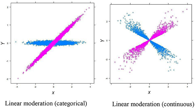
Figure 1. Diagrams that show linear moderations (with a categorical moderator M on the left and a continuous moderator M on the right). The blue dots are the selected cases with a lower value in M [i.e., M = 0 for the categorical moderation, and M = −1 (1 SD below mean) for the continuous moderation]. The purple does are the selected cases with a higher value in M [i.e., M = 1 for the categorical moderation, and M = 1 (1 SD above mean) for the continuous moderation].

Undoubtedly, examining linear moderations (either categorical or continuous) is a necessary but not sufficient practice in many research studies that examine human behaviors. For instance, in cognitive psychology, Yerkes and Dodson [4] developed the well-known Yerkets-Dodson Law, which empirically explains that the relationship between psychological arousal and performance forms an inverted U shape (curvilinear relationship), meaning that performance only increases with psychological arousal until a certain threshold, and beyond that, performance decreases with increasing arousal. In health sciences, the most optimal health status or outcome (Variable Y) is often observed at middle points of many predictors Xs (e.g., heart rate, blood pressure, weight), and hence, X and Y also form an inverted U shape pattern. In those cases, fitting a linear slope between X and Y will result in a slope of zero, which cannot signal and detect the true underlying curvilinear relationship between X and Y. As extension, we cannot detect curvilinear moderation, the extent to which the curvilinear relationship between X and Y varies across the levels of a moderator. Indeed, [5], one of the pioneers who proposed mediation and moderation analysis in psychological research, suggested that researchers may wish to examine whether quadratic or curvilinear moderation exists in their data. However, Jose [6] found that curvilinear moderation has received far less attention than linear moderation for a number of reasons. First, researchers usually do not consider and specify quadratic hypotheses to test curvilinear relationships. Jose stated that “this is a shame” (p. 214), given that many curvilinear relationships indeed exist in behavioral data. Second, researchers typically do not know how to conduct a quadratic- or curvilinear-moderation analysis in a statistical package (e.g., SPSS). Third, the existing statistical packages often do not offer clear guidelines for researchers to quickly assess and visualize data that contains curvilinear relationships.

In light of the importance of moderation analysis and the lack of attention to curvilinear moderation in the literature, I describe eight different types of nonlinear moderation that behavioral researchers may often encounter in their research, and propose algorithms for estimating the point estimates, constructing the corresponding confidence intervals, and calculating the associated p-values for testing these curvilinear moderations. I conducted a Monte Carlo simulation study to compare the results of standard linear moderation analysis to the curvilinear moderation analysis procedures that I propose.

This paper is organized into four sections. In Section 1, I review the background of linear moderation and describe curvilinear moderation models. In Section 2, I discuss the design of the simulation study and I present the simulation results in Section 3. Then, in Section 4, I discuss the implications of the findings and the importance of curvilinear moderation in behavioral research.

Background of Linear and Curvilinear Moderations

Linear Moderation (Categorical and Continuous)

In the framework of multiple regression, a linear moderation can be expressed as

where Y_i is an observed score for respondent i = 1, 2, …, n from the regression model in Equation (1), X_i is the predictor X score for respondent i, M_i is the moderator M score for respondent i, _XiMi is the multiplicative score between X and M for respondent i (i.e., moderation effect), b₀ is the intercept term, b₁ is the regression slope for predictor X, b₂ is the regression slope for moderator M, b₃ is the regression slope for the interaction term _XiMi, and _eYi is the residual score. For simplicity, the subscript i in (1) is dropped, and the equation becomes Y = b₀ + b₁X + b₂M + b₃XM + e_Y.

It is important to note that, in practice, X_i and M_i scores in Equation (1) are often substituted by their centered scores, i.e., $X_{c_i}=X_i-\overline{X}$ and $M_{c_i}=M_i-\overline{M}$, where $\overline{X}$ is the mean of all X scores and $\overline{M}$ is the mean of all M scores, for a number of reasons. First, X and M may not have a meaningful zero value (e.g., continuous X is body weight, continuous M is age, and categorical M is age group with two levels: young children of 3–6 years and old children of 7–10 years), and hence, examining the effect of X when M = 0 is meaningless. Second, multiplying raw X and M scores will likely to produce unrealistic large interaction/moderation scores (i.e., XM; e.g., X is calendar year and M is household income) that could lead to math overflow in estimation. Third, centering X and M could mitigate the issue of multicollinearity between higher-order predictors (for details regarding centering or not-centering predictors, please refer to Aiken and West [7], Cohen et al. [8]. In this study, without restricting the applicability of curvilinear algorithms to centered X and M scores only, the following equations are presented based on the generic terms of X and M, and researchers can decide whether they have to center their X and M scores in practice.

In most research situations, researchers often plot their data for better understanding moderation effects. When M is categorical, a regression line can be plotted to regress Y on X for the first and second groups, respectively. When M is continuous, there are two common approaches for categorizing continuous linear moderation for better visualization. A first approach is known as the “pick a point” approach [8–10], in which researchers arbitrarily choose two (or more values) in M (e.g., 1 SD above and below the mean of M). A second approach is known as the Johnson-Neyman approach (J-N; [3, 11, 12]), in which researchers estimate a range of values in M (based on discriminant function analysis) so that these values can maximize the differences in the conditional effects (or simple slopes) that regress Y on X. The rationale is that researchers should focus on the critical M values (e.g., personality trait) that substantially and significantly change the (simple) slope values regressing Y (e.g., performance) on X (e.g., work pressure), which is important for theory and model testing in behavioral sciences. For example, Hofmans et al. [13] stated that the existing literature often focused on linear moderation, and hence, they examined if there exists any curvilinear relationship between work pressure and momentary task performance, and how this relationship can be moderated by one's personality trait (e.g., core self-evaluations [CSE], i.e., one's appraisals about self-worth, capabilities, and competency). They found that people with a high level of CSE are less affected by work pressure (i.e., a more flattened, inverted U shape between pressure and performance) than people with a low level of CSE (i.e., a more leptokurtic, inverted U shape between pressure and performance). Indeed, Hofmans et al.'s scatterplot (Figure 2, p. 7) between work pressure and performance separated by high and low CSE (±1 SD) appears to be identical to the proposed Model 8 (Figure 2) in the present study with the blue points belong to the high CSE group, and the purple points belong to the low CSE group.

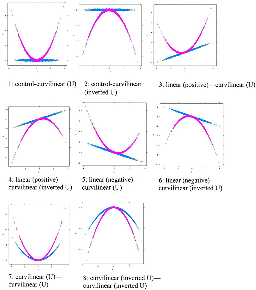
Figure 2. Eight types of Curvilinear Moderations (Categorical). The blue line shows the group of observations with a lower score in the moderator M (i.e., Group 0). The purple line shows the group of observations with a higher score in the moderator M (i.e., Group 1).

Curvilinear Moderation (Categorical and Continuous)

As noted above, there are a number of behavioral phenomena that involve bivariate relationships that are nonlinear or curvilinear (e.g., psychological arousal and performance). If a researcher fits a linear moderation model for these phenomena, the researcher will be unable to appropriately detect the underlying true curvilinear moderation. Failing to identify the true nature of the relationship poses a serious threat to the accuracy of theory testing and to the validity of implications of the findings. Based on the literature related to the inverted U-shape curve between stress and performance, Li's [14] paper summarized the algorithms and discussed the potential applications of curvilinear moderation in behavioral sciences. Specifically, Li concluded that there are eight common types of curvilinear moderations that researchers should consider in their research studies (shown in Figure 2). Li suggested that appropriate re-analysis of existing data-sets in behavioral sciences could reveal previously undetected curvilinear moderations of significant impact in behavioral science research. Despite the substantial implication of this work, Li's paper did not systematically and comprehensively compare and evaluate the results between linear and curvilinear moderations in a Monte Carlo simulation study. Moreover, the conceptual and computational details of these eight common types of curvilinear moderations were not included, which prevents researchers and practitioners to use and follow the procedures in conducting curvilinear-moderation analysis.

In the framework of multiple regression, a full model for curvilinear moderation can be expressed as

where Y_i, b₀, X_i, M_i, and e_Yi are defined in Equation (1), $X_i^2$ is the square of X_i for respondent i, b_j (where j = 1, 2 …, 7) is the regression slope that relates Y to the corresponding effect (e.g., X_i). Specifically, there are three main effects (i.e., $b_1{X}_i+b_2{M}_i+b_3{X}_i^2$), three two-way moderation effects (i.e., all possible two-way multiplications for X_i, M_i, and $X_i^2$: $b_4{X}_i{M}_i+b_5{X}_i^2{M}_i+b_6{X}_i^3$), and one three-way moderation effect (i.e., $b_7{X_i^{3}M}_i$). For simplicity, the subscript i is dropped, and (2) becomes $Y=b_0+b_{1}X+b_{2}M+b_3{X}^2+b_{4}XM+b_5{X}^{2}M+b_6{X}^3+b_7{X}^{3}M+e_Y$.

Statistically speaking, there exists many different combinations of b_j (where j = 1, 2 …, 7) in (2) leading to many different patterns of curvilinear moderations. For simplicity and better visualization, M is conceptualized as a binary or categorical moderator (or as a two-group moderator with 1 SD above and below the mean of a continuous M based on the “pick a point” approach) in Figure 2, so that a regression line for X-Y can be shown for each of the group labels of the moderator M. To make the conceptual meaning clear I hereafter refer to each type of curvilinear moderations as a pattern1—pattern 2 moderation, where pattern 1 refers to the pattern of relationship between X and Y [i.e., control, linear (positive and negative), curvilinear (U and inverted U)] for M = 1, and pattern 2 indicates the pattern of relationship between X and Y [i.e., control, linear (positive and negative), curvilinear (U and inverted U)] for M = 2.

Categorical Curvilinear Moderation

Type 1 is a control-curvilinear (U) moderation, in which X-Y shows no pattern of relationship (i.e., control) in Group 1, whereas X-Y follows a curvilinear (U shaped) relationship in Group 2 (Figure 2, Panel 1). For ease of understanding, the intercept b₀ is assumed to be zero, and the slope parameter value is assumed to be 1 if an effect exists, and 0 if an effect does not exist. The full model in Equation (2) can in this case be simplified as

Type 2 is a control-curvilinear (inverted U) moderation, and is different from Type 1 only with respect to the fact that the curvilinear relationship in Group 2 is an inverted U shape (Figure 2, Panel 2). The full model in (2) can be simplified for Type 2 as

Types 3 through 6 are all linear-curvilinear moderations, in which Group 1 follows a linear relationship between X and Y, and Group 2 adheres to a curvilinear relationship between X and Y. Specifically, Type 3 is a linear (positive)—curvilinear (U) moderation, in which X and Y follows a positive linear relationship in Group 1, and they form a U-shape relationship in Group 2. The Type 3 model can be expressed as

Type 4 is a linear (positive)—curvilinear (inverted U) moderation, expressed as

Type 5 is a linear (negative)—curvilinear (U) moderation, expressed as

Type 6 is a linear (negative)—curvilinear (inverted U) moderation, expressed as

The remaining two types are both known as a curvilinear—curvilinear moderation, in which the degree and extent curvilinearity in the relationship between X and Y differs between Groups 1 and 2. Specifically, Type 7 is a curvilinear (U)—curvilinear (U) moderation, expressed as

Type 8 is a curvilinear (inverted U)—curvilinear (inverted U) moderation, expressed as

Continuous Curvilinear Moderation

The eight types of continuous moderations follow the same Equations (3) to (10) except that the moderator M becomes a continuous variable. With a continuous M, the shapes of the curvilinear moderation may look quite different from those found in categorical curvilinear moderation. For better visual presentation, the shapes of the continuous curvilinear moderations are shown in Figure 3 based on the “pick-a-point” method with 1 SD above or below the mean. Type 1 is a curvilinear (inverted U)—curvilinear (U) moderation, and Type 2 is a curvilinear (U)—curvilinear (inverted U) moderation. Types 3 and 4 look similar to Types 1 and 2 with the exception the U and inverted U curves show an increasing trend or pattern when predictor X increases, and they are called a positive curvilinear (U or inverted U)—curvilinear (inverted U or U) moderation. By the same token, Types 5 and 6 appear to be similar to Types 1 and 2, except for the fact that the U and inverted U curves show a decreasing trend with increasing X values, and they are called a negative curvilinear (U or inverted U)—curvilinear (inverted U or U) moderation. Types 7 and 8 appear to be similar to the control-curvilinear (U) and control-curvilinear (inverted U) types in continuous moderation, in which the scores in one group (either 1 SD below or above the mean) adhere to a smaller degree of curvilinearity and the scores in another group (either 1 SD above or below the mean) have a larger extent of curvilinearity.

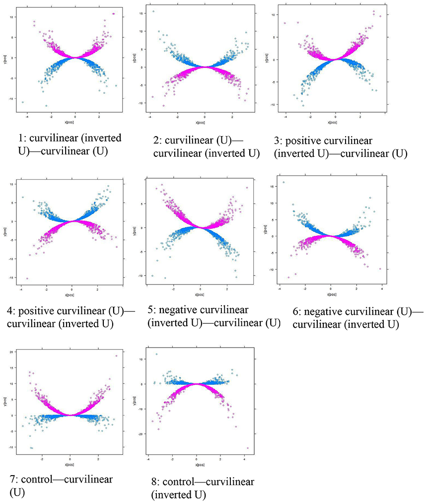
Figure 3. Eight types of Curvilinear Moderations (Continuous). The blue line shows the group of observations with a lower score in the moderator M (i.e., 1 SD below mean in continuous moderation). The purple line shows the group of observations with a higher score in the moderator M (i.e., 1 SD above mean in continuous moderation).

Practical Consideration

Comparing (2) to (1), it is clear that linear moderation in Equation (1), which is the state-of-the-art practice in behavioral research, is only a special case of the curvilinear moderation in Equation (2). That is, if and only if b₃, b₅, b₆, and b₇ are zeros, and b₄ (and/or b₁ and b₂) is different from zero in Equation (2), then the curvilinear moderation will simplify to the linear moderation in Equation (1). In practice, a researcher can start from a full curvilinear moderation model in Equation (2). When any of the aforementioned curvilinear-moderation types is an appropriate model for the true underlying relationship in the population, a researcher can appropriately detect this based on Equation (2). When linear moderation is the true relationship in population, a researcher can also detect this moderation in Equation (2) with the expected values of zeros for b₃, b₅, b₆, and b₇, and the expected non-zero values for b₄ (and/or b₁ and b₂). It is important to that when this method is used to detect a linear moderation there is some loss of degrees of freedom as compared to the traditional approach because of the increased number of estimated parameters, which in turn result in a less powerful test for regression slopes. On the other hand, the risk is even higher if a researcher fits an inappropriate linear-moderation model for variables that truly have curvilinear relationships at the population level, because such analysis will lead to an incorrect conclusion being drawn about the nature of the moderation.

Monte Carlo Simulation

The primary purpose of conducting a Monte Carlo simulation study is to evaluate whether the statistical results based on curvilinear moderation are accurate and trustworthy across different data situations—including eight types of curvilinear moderation, sample sizes, proportion of variance explained (or goodness-of-fit) of a curvilinear-moderation model, and binary/continuous moderator effect—that most behavioral researchers are facing and dealing with in practice. The secondary purpose is to evaluate how researchers may miss or misidentify any important curvilinear moderations if they only conduct the conventional linear-moderation analysis. As in most other Monte Carlo simulations involving moderation effects (e.g., [15]), there is no way for us to include and manipulate all possible levels of moderation effects. Rather, the current simulation examines five factors: curvilinear type, sample size, proportion of variance explained, type of moderator, and sample size ratio between two groups (for categorical moderator only), which is considered comprehensive in simulating real-world situations. Given that researchers often evaluate point estimates of regression slopes and multiple correlation squared (i.e., R²; proportion of variance of Y accounted for by all the predictors in a regression model), the associated significance (p-values), and confidence intervals, I have evaluated performance of each model by measuring the accuracy of these statistical estimates under each model.

Design

Factor 1 (Curvilinear Type θ; 8 Levels)

A shown in Table 1, the slope parameters were fixed at zero if they are not supposed to be related to the outcome measure Y. On the other hand, for the slope parameters that should be associated with the outcome measure Y, their values were manipulated at 0.5 to mimic a research scenario in which an effect exists for each of the eight types of curvilinear moderation. Take Type 3 [linear (positive)—curvilinear (U) moderation] as an example: b₁ and b₅ were fixed at 0.5, whereas b₂, b₃, b₄, b₆, and b₇ were set at 0.

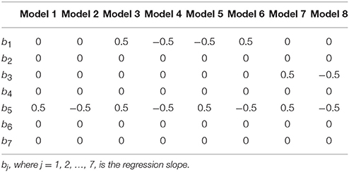
Table 1. Slope parameters manipulated in the simulation study.

Factor 2 (Sample Size n; 6 Levels)

Six levels−50, 100, 150, 200, 250, and 500—were evaluated, which is sufficient to cover the range of sample sizes, from a small to large, that are common in most behavioral research scenarios.

Factor 3 (R Squared R²; 5 Levels)

Five levels−0.1, 0.2, 0.3, 0.4, 0.5—were examined. In behavioral research, predictors in a regression model always explain less than 100% of the variance of the criterion Y. In this study, this proportion was manipulated at 10, 20, 30, 40, and 50%, which covers the range of small to large effect sizes (proportion of variance explained) according to Cohen [16].

Factor 4 (Type of Moderator γ; 2 Levels)

Two types—continuous and categorical (binary)—were manipulated, which are typically found in behavioral research.

Factor 5 (Sample Size Ratio π; 3 Levels)

For categorical moderation in Factor 4, three levels of sample size ratio between two groups−0.25, 0.5, 0.75—were evaluated. n₁ refers to the sample size in Group 1 (i.e., M = 1), and n₂ is the sample size in Group 2 (i.e., M = 2). Thus, n·π = n₁ and n·(1 − π) = n₂. This mimics the common research scenario of having different sample sizes for the two groups labeled in the moderator M.

In sum, this study addresses a design with 8 × 6 × 5 × 3 = 720 conditions for a categorical moderator and a design with 8 × 6 × 5 = 240 conditions for a continuous moderator. Each of the 960 conditions was replicated 10,000 times to evaluate their overall performance across replications, thereby generating a total of 9,600,000 simulated samples. The code for this simulation was executed in R Studio [17], and is shown in Supplementary Data Sheet 1.

Regarding data generation, for each of the 960 simulation conditions, continuous X and continuous M were first generated from a normal distribution with a mean of 0 and a SD of 1. For categorical M, n₁ numbers of 0 were randomly generated from a sample (without replacement) of size n to indicate the first group, and the remaining numbers were assigned to be 1 to indicate the second group. Second, the simulated X and M scores were centered in order to mitigate the issue of multicollinearity among higher-order predictors, and to avoid the unrealistic interpretation of the effect of X on Y when M = 0 (e.g., age = 0) that may not exist in practice. Third, given that the (centered) X and M scores were known, the scores for other predictors (i.e., X², X³, XM, X²M, and X³M) were also computed. Fourth, for ease of manipulation, the intercept term b₀ was set at 0. Fifth, given all the generated scores from all the predictors (i.e., X, M, X², XM,X²M, X³, and X³M), these scores were multiplied by the manipulated slope parameters (i.e., b₁, b₂, …, b₇ in Factor 1) to generate the true Y scores through Equation (2). Sixth, to introduce residual variance, e_Y scores were added to the true Y scores (Y^t) to become the observed Y scores (i.e., Ŷ), where e_Y were generated from a normal distribution with a mean of 0 and a SD of $\sqrt{\frac{Var(Y^t)}{R^2}-Var(Y^t)}$,¹ so that the expected proportion of variance explained in the simulated regression model equals the value manipulated in Factor 3.

In this study, I extract common statistical results that researchers are often interested in and can extract from the widely-employed function (lm) in R. Specifically, sample estimates—including slope estimates (i.e., b_j, where j = 1, 2, …, 7) and proportion of variance explained estimates (i.e., R² and $R_{adj}^2$)—in curvilinear moderation are examined in this study. In addition to these point estimates, researchers often report and interpret statistical significance (i.e., p < 0.05) and the confidence intervals (CI) surrounding these point estimates. Hence, the Type 1 error and Power rates of b_j and R² from which we can infer statistical significance, and the coverage probability used to examine the performance of the CI, are also evaluated.

Evaluation Criteria

The purpose of this evaluation is to examine whether or not the point estimates for b_j, R², and $R_{adj}^2$ based on curvilinear moderation (Equation 2) are accurate across the 960 simulation conditions. Moreover, this evaluation assesses whether or not the 95% CI surrounding these estimates would lead to appropriate results of Type I error, Power, and coverage probability.

Absolute Bias (AB) and Mean Absolute Bias (MAB)

AB is defined as the absolute difference between the mean of the 10,000 δ replicated estimates (denoted as $\overline{\delta }$, including b_j, R², and $R_{adj}^2$), and Δ is the associated true parameter value in population, i.e., $\lceil \overline{\delta }-\Delta \rceil$. According to Algina and Keselman [18], one can evaluate the number of ABs that are within the criterion of 0.025 and 0.05 across 960 conditions. To summarize the overall performance across 960 conditions, MAB can be computed as $\sum _{i=1}^{960}\frac{AB(i)}{960}$.

Type I Error and Power

Type I error rate is used to evaluate how likely a sample estimate (e.g., b_j, R²) is considered statistically significant at the 0.05 level, if its true population value is zero. Given that the Type I error rate is often set a priori at 0.05 in behavioral research, the ideal number of significant results (p < 0.05) to be observed out of the 10,000 replicated p values associated with their sample estimates is 500 (or 5%). Power is defined as the likelihood that a sample estimate is considered statistically significant at the 0.05 level given that its true population value is different from zero. Of the 10,000 replicated p-values associated with their sample estimates, in theory, the number of significant p values should be as close to 10,000 as possible (or Power rate = 100%). However, this rate never reaches 100% unless one has an infinite sample size (i.e., asymptotic theory). In practice, it is common for researchers to design their studies with the target of achieving an 80% Power rate. Hence, in this study, the Power rates across 960 manipulated conditions are evaluated, and a relatively higher rate means a more appropriate procedure, meaning that this procedure leads to a correct decision to reject the null hypothesis that a true parameter value is zero.

Coverage Probability

Coverage probability is defined as the likelihood that the true parameter value is found within the span of the lower and upper limits of the CI across 10,000 replications. Given that 95% CI is often used in behavioral research, ideally, the number of replications in which the true value should be found within the CI is expected to be 9,500 out of 10,000 replications (or 95%). In practice, there exists sampling error for the observed coverage probability in a simulation study. According to [19], an observed coverage probability is considered accurate, if it falls within the region of [0.9444, 0.9556], given that the 99% sampling interval for the observed coverage probability (i.e., 0.95) across 10,000 replications is approximately $0.95\pm 2.576\sqrt{\frac{(0.95)(0.05)}{10,000}}$.

Results

MAB (Table 2)

Linear Moderation

The results of linear moderation analysis were found to be inaccurate. The ABs for the b₂ estimates were the least desirable, and ranged from 0.369 to 0.507 (M = 0.480, SD = 0.019). In this simulation, the true parameter value for b₂ was fixed at zero, and there is a mean absolute bias of 0.480 between these sample estimates and the true value. Of the 960 conditions, none (or 0%) of the estimated b₂ values were within the criteria of 0.025 and 0.05. This is probably due to the lack of the actual slope parameter b₅ (for predictor X²M) in linear moderation, and hence, its effect can only (and inappropriately) be captured through another slope parameter b₂ (for moderator M). The sample estimates, R squared and adjusted R squared, that evaluate the proportion of variance explained in the regression model were also found to be inaccurate. The ABs for R squared ranged from 0.000 to 0.456 (M = 0.137, SD = 0.110). Of the 960 conditions, only 110 (or 11.5%) of the R squared estimates were within the criterion of 0.025, and 236 (or 24.6%) were within the criterion of 0.05. The ABs for adjusted R squared estimates were also inadequate, ranging from 0.021 to 0.462 (M = 0.156, SD = 0.110). Of the 960 conditions, only 48 (or 5.0%) of the adjusted R squared estimates were within the criterion of 0.025, and 114 (or 15.0%) were within the criterion of 0.05. The remaining estimates, b₁ and b₃, were found to be reasonable.

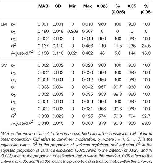
Table 2. Absolute biases of the parameter estimates.

Curvilinear Moderation

Under curvilinear-moderation analysis the performances of the b_j (j = 1, 2, .., 7) estimates were found to be highly accurate, as shown in Table 2. Their MABs were all very small, ranging from 0.001 to 0.003 (M = 0.002), indicating an excellent fit. Of the 960 conditions, the number of conditions with a b_j estimate within the stringent criterion of 0.025 were also appropriate, ranging from 957 to 960 (or 99.7 to 100%), with a mean of 959 (or 99.9%). For a more lenient criterion of 0.05, the results were perfect, with 960 (or 100%) conditions yielding a bias less than 0.05. Comparing R squared with adjusted R squared, the adjusted R squared results were more accurate. The ABs ranged from 0.000 to 0.060 (M = 0.010, SD = 0.010). Of the 960 conditions, 873 (or 90.9%) of the adjusted R squared estimates fell within the stringent criterion of 0.025, and 950 (or 99.0%) of the adjusted R squared estimates were within the lenient criterion of 05. In sum, these results indicate that reporting the b_j (j = 1, 2, .., 7) and adjusted R squared estimates appears to be an accurate and highly desirable practice for evaluating the effects under curvilinear moderation.

Type I Error and Power (Table 3)

Linear Moderation

The Type 1 error rates were less than optimal for the linear moderation analysis. As noted above, given that the effect of curvilinear moderation can only be captured through the main effect of the moderator (b₂), the b₂ estimates are often higher than the true value of 0. Hence, the error rates of b₂ were much higher than the true value (0.05), ranging from 0.081 to 1.000 (M = 0.701, SD = 0.290). The error rates for b₁ and b₃ were also less than satisfactory, with a mean of 0.130 for b₁ and a mean of 0.158 for b₃. Regarding Power, only b₁ and R squared yielded satisfactory Power rates (0.909 and 0.799).

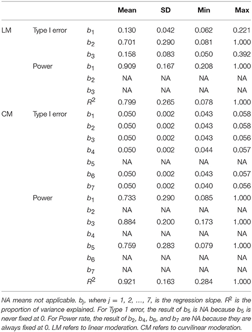
Table 3. Type I error and Power rates.

Curvilinear Moderation

The means of the Type 1 error rates were excellent (0.050) for all the slope parameter values of b₁, b₂, b₃, b₄, b₆, and b₇. The mean Power rate was excellent for the R squared (0.921), good for b₃ (0.884), b₅ (0.759), and b₁ (0.733). These results show that the estimations based on curvilinear moderation are appropriate for researchers to better understand the true relationships between the IVs and DVs in their research.

Coverage Probability (Table 4)

Linear Moderation

The coverage probability of b₂ was poor with a mean of 0.299 and a SD of 0.290. The minimum coverage probability could also be as low as 0 across 10,000 replications, which is highly unsatisfactory. Of the 960 conditions, 0 (or 0%) of the CI of b₂ spanned its true parameter value. This result is understandable because, as noted above, there is no parameter that captures the degree of curvilinear moderation, and hence, this degree can only be mistakenly reflected and measured by b₂. The means of the coverage probabilities for b₁ and b₃ were slightly better (0.885 and 0.842), but they were still notably smaller than the true value of 0.95. Of the 960 conditions, only 2 (or 0.2%) and 16 (or 1.7%) fell within the criteria of [0.9444, 0.9556], respectively.

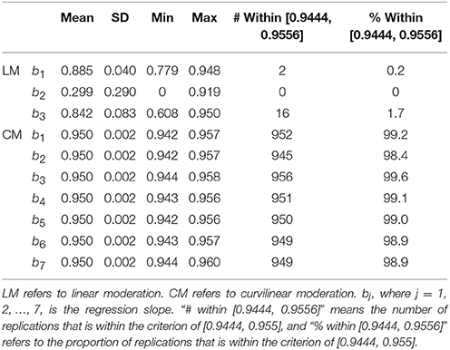
Table 4. Coverage probabilities across 960 simulation conditions.

Curvilinear Moderation

All the coverage probabilities were excellent (0.950) for b_j (j = 1, 2, …, 7). These probabilities ranged from 0.942 to 0.960, which is highly desirable. Across 960 simulation conditions, the numbers of inclusion of the true parameter value ranged from 945 to 956 (or 98.4 to 99.6%) for the CIs surrounding b_j (j = 1, 2, .., 7), which is also an excellent fit.

Conclusion and Discussions

Curvilinear relationship between two variables (X and Y) is arguably one of the most important patterns of relationship beyond linear relationship in behavioral sciences. Discussion of curvilinear relationship in the behavioral sciences can be traced back at least to the early 1900s when Yerkes and Dodson [4] identified a widely employed curvilinear relationship between psychological arousal and performance, which is well known as the Yerkes-Dodson Law in psychology. Despite the importance of curvilinear relationship, it comes as some surprise that curvilinear moderation—a statistical model that identifies differences in the strength and direction of curvilinearity between X and Y across the levels of M—is neither commonly used by researchers nor has it received the attention in the literature that it deserves. As noted in Hofmans et al. [13], the inverted U shape between work pressure and performance may differ across different personality traits (e.g., high versus low CSE). Afshar et al. [20] further found that people with maladaptive personality traits (e.g., neuroticism) tend to form a more flattened, inverted U-shape relationship between stress and performance, whereas people with adaptive personality traits (e.g., openness) tend to form the usual inverted U shape between stress and performance as stated in the Yerkets-Dodson Law. These findings suggest that researchers should examine curvilinear relationships in order to better understand the curvilinear patterns of relationships in behavioral research. The curvilinear-moderation method proposed in this study provides a good solution to Jose's [6] criticism that researchers should often specify quadratic hypotheses to test curvilinear relationships. The computational details of the eight curvilinear algorithms that correspond to the visual scatterplots (Figures 2, 3) also help researchers understand when they should consider curvilinear moderations, and how they could specify the higher-order slope effects in their regression model.

The current simulation results clearly show how detrimental the analytic results could be if a researcher fits an inappropriate linear moderation model to data that, in fact, come from a curvilinear moderation in the population. For instance, a researcher may misinterpret that a continuous moderator M (e.g., intelligence) can significantly and linearly predict a dependent variable (e.g., performance), or there is only a significant mean difference of intelligence between the levels of a categorical moderator M (e.g., males and females). Such a misidentification is detrimental for theory and model testing, not only in understanding the true underlying psychological process or mechanism in human beings, but it is harmful for practitioners (e.g., policy makers, human resources managers, educators, psychologists) when they make policies, hire job applicants, or develop interventions programs for individuals.

This study also systemically outlines the algorithms (Equations 3 to 10) and provides intuitive visualizations of each of the curvilinear patterns in Figures 2, 3, with the goal to increase researchers' awareness of how patterns of relationship in their datasets should look if there exists any curvilinear moderations. I believe that conducting a preliminary visual search (i.e., scatterplots for all bivariate relationships) for curvilinear patterns and comparing the proportions of variance explained (e.g., R² or $R_{adj}^2$) based on linear and curvilinear moderations, a practice worth recommending to researchers who explore variables with which curvilinear moderations may exist.

Limitations and Future Directions

A first direction for future research involves extending the approach I have used in this study to additional types of curvilinear moderations that could be encountered in behavioral research. This study offers eight potentially common and important types of curvilinear moderations for researchers to consider as a starting point. As an extension, there exist more complex types of curvilinear moderations (e.g., three-way curvilinear moderations involving one X and two curvilinear moderators). A second direction lies in conceptualizing the errors or residuals of the curvilinear-moderation models. In this study, errors or residuals were assumed to be independent of the effects in the models, and were randomly generated from a normal distribution with a mean of 0 and a SD of $\sqrt{\frac{Var(Y^t)}{R^2}-Var(Y^t)}$, in which Var(Y^t) was approximated by the mean of 10,000 simulated variances of Y scores without error terms (i.e., M[s²(Y^t)] in Footnote 1). In the future, additional research could introduce a multi-level or mixed-effects approach, in which some of the slope parameters (i.e., X or M) are assumed to be random-effects so that the residuals or errors can be correlated with some of the slope values, in order to provide a more complete picture of curvilinear moderations in behavioral research.

Author Contributions

JL is the sole author, who is responsible for reviewing the literature, designing the simulation study, and interpreting the simulation results for this research study.

Conflict of Interest Statement

The author declares that the research was conducted in the absence of any commercial or financial relationships that could be construed as a potential conflict of interest.

Supplementary Material

The Supplementary Material for this article can be found online at: https://www.frontiersin.org/articles/10.3389/fams.2018.00007/full#supplementary-material

Footnotes

References

1. Sigley R. The importance of interaction effects. Lang Variat Change (2003) 15:227–53. doi: 10.1017/S0954394503152040
2. John LK, Loewenstein G, Prelec D. Measuring the prevalence of questionable research practices with incentives for truth telling. Psychol Sci. (2012) 23:524–32.
3. Hayes A. Introduction to Mediation, Moderation, and Conditional Process Analysis: A Regression-Based Approach. New York, NY: Guilford (2013).
4. Yerkes RM, Dodson JD. The relation of strength of stimulus to rapidity of habit-formation. J Comp Neurol Psychol. (1908) 18:459–82. doi: 10.1002/cne.920180503
5. Baron RM, Kenny DA. The moderator-mediator variable distinction in social psychological research: conceptual, strategic and statistical considerations. J Personal Soc Psychol. (1986) 51:1173–82.
7. Aiken LS, West SG. Multiple Regression: Testing and Interpreting Interactions. Newbury Park, CA: Sage (1991).
8. Cohen J, Cohen P, West S, Aiken L. Applied Multiple Regression / Correlation Analysis for the Behavioral Sciences, 3rd Edn. Mahwah, NJ: Lawrence Erlbaum (2003).
9. Bodner T. Tumble graphs: avoiding misleading end point extrapolation when graphing interactions from a moderated multiple regression analysis. J Educ Behav Statist. (2016) 41:593–604. doi: 10.3102/1076998616657080
10. Dawson J. Moderation in management research: what, why, when and how. J Bus Psychol. (2014) 29:1–19. doi: 10.1007/s10869-013-9308-7
11. Bauer D, Curran P. Probing interactions in fixed and multilevel regression: inferential and graphing techniques. Multivar Behav Res. (2005) 40:373–400. doi: 10.1207/s15327906mbr4003_5
12. Johnson P, Neyman J. Tests of certain linear hypotheses and their application to some educational problems. Statis Res Mem. (1936) 1:57–93.
13. Hofmans J, Debusscher J, Doci E, Spanouli A, De Fruyt F. The curvilinear relationship between work pressure and momentary task performance: the role of state and trait core self-evaluations. Front Psychol. (2015) 6:1680. doi: 10.3389/fpsyg.2015.01680
14. Li JC-H. Nonlinear moderation. In: Paper Presented at the 2016 International Meeting of Psychometric Society. Asheville, NC (2016).
15. Cheung MW-L. Comparison of approaches to constructing confidence intervals for mediating effects using structural equation models. Struct Equat Model Multidiscipl J. (2007) 14, 227–46.
16. Cohen J. Statistical Power Analysis for the Behavioral Sciences, 2nd edn. Hillsdale, NJ: Lawrence Erlbaum (1988).
17. R Studio Team. R Studio: Integrated Development for R. Boston, MA: R Studio, Inc. (2017). Available online at: http://www.rstudio.com
18. Algina J, Keselman HJ. Cross-validation sample sizes. Appl Psychol Meas. (2000) 24:173–9. doi: 10.1177/01466210022031606
19. Chan W, Chan DW-L. Bootstrap standard error and confidence intervals for the correlation corrected for range restriction: a simulation study. Psychol Methods (2004) 9:369–85. doi: 10.1037/1082-989X.9.3.369
Keywords: curvilinear moderation, linear moderation, Monte Carlo study, regression models, simple slope effects
Citation: Li JC-H (2018) Curvilinear Moderation—A More Complete Examination of Moderation Effects in Behavioral Sciences. Front. Appl. Math. Stat. 4:7. doi: 10.3389/fams.2018.00007
Received: 19 July 2017; Accepted: 15 March 2018;
Published: 06 April 2018.
Edited by:
Holmes Finch, Ball State University, United StatesReviewed by:
Shu Fai Cheung, University of Macau, ChinaShevaun D. Neupert, North Carolina State University, United States
Copyright © 2018 Li. This is an open-access article distributed under the terms of the Creative Commons Attribution License (CC BY). The use, distribution or reproduction in other forums is permitted, provided the original author(s) and the copyright owner are credited and that the original publication in this journal is cited, in accordance with accepted academic practice. No use, distribution or reproduction is permitted which does not comply with these terms.
*Correspondence: Johnson Ching-Hong Li, johnson.li@umanitoba.ca