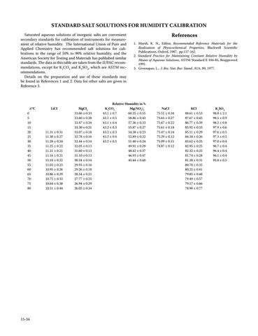
STANDARD SALT SOLUTIONS FOR HUMIDITY CALIBRATION Saturated aqueous solutions of inorganic salts are convenient secondary standards for calibration of instruments for measurement of relative humidity. The International Union of Pure and Applied Chemistry has recommended salt solutions for calibrations in the range of 10% to 90% relative humidity, and the American Society for Testing and Materials has published similar standards. The data in this table are taken from the IUPAC recommendations, except for K2CO3 and K2SO4, which are ASTM recommendations. Details on the preparation and use of these standards may be found in References 1 and 2. Data for other salts are given in Reference 3.
t/°C
0 5 10 15 20 25 30 35 40 45 50 55 60 65 70 75 80
LiCl
11.31 ± 0.31 11.30 ± 0.27 11.28 ± 0.24 11.25 ± 0.22 11.21 ± 0.21 11.16 ± 0.21 11.10 ± 0.22 11.03 ± 0.23 10.95 ± 0.26 10.86 ± 0.29 10.75 ± 0.33 10.64 ± 0.38 10.51 ± 0.44
MgCl2 33.66 ± 0.33 33.60 ± 0.28 33.47 ± 0.24 33.30 ± 0.21 33.07 ± 0.18 32.78 ± 0.16 32.44 ± 0.14 32.05 ± 0.13 31.60 ± 0.13 31.10 ± 0.13 30.54 ± 0.14 29.93 ± 0.16 29.26 ± 0.18 28.54 ± 0.21 27.77 ± 0.25 26.94 ± 0.29 26.05 ± 0.34
References 1. Marsh, K. N., Editor, Recommended Reference Materials for the Realization of Physicochemical Properties, Blackwell Scientific Publications, Oxford, 1987, pp.157-162. 2. Standard Practice for Maintaining Constant Relative Humidity by Means of Aqueous Solutions, ASTM Standard E 104-85, Reapproved 1991. 3. Greenspan, L., J. Res. Nat. Bur. Stand., 81A, 89, 1977.
Relative Humidity in % K2CO3 Mg(NO3)2 43.1 ± 0.7 60.35 ± 0.55 43.1 ± 0.5 58.86 ± 0.43 43.1 ± 0.4 57.36 ± 0.33 43.2 ± 0.3 55.87 ± 0.27 43.2 ± 0.3 54.38 ± 0.23 43.2 ± 0.4 52.89 ± 0.22 43.2 ± 0.5 51.40 ± 0.24 49.91 ± 0.29 48.42 ± 0.37 46.93 ± 0.47 45.44 ± 0.60
NaCl 75.51 ± 0.34 75.65 ± 0.27 75.67 ± 0.22 75.61 ± 0.18 75.47 ± 0.14 75.29 ± 0.12 75.09 ± 0.11 74.87 ± 0.12
KCl 88.61 ± 0.53 87.67 ± 0.45 86.77 ± 0.39 85.92 ± 0.33 85.11 ± 0.29 84.34 ± 0.26 83.62 ± 0.25 82.95 ± 0.25 82.32 ± 0.25 81.74 ± 0.28 81.20 ± 0.31 80.70 ± 0.35 80.25 ± 0.41 79.85 ± 0.48 79.49 ± 0.57 79.17 ± 0.66 78.90 ± 0.77
K2SO4 98.8 ± 2.1 98.5 ± 0.9 98.2 ± 0.8 97.9 ± 0.6 97.6 ± 0.5 97.3 ± 0.5 97.0 ± 0.4 96.7 ± 0.4 96.4 ± 0.4 96.1 ± 0.4 95.8 ± 0.5
15-34
Section 15.indb 34
5/3/05 9:12:00 AM
LOW TEMPERATURE BATHS FOR MAINTAINING CONSTANT TEMPERATURE A liquid-solid slurry is a convenient means of maintaining a constant temperature environment below room temperature. The following is a list of readily available organic liquids suitable for
this purpose, arranged in order of their melting (freezing) points tm. The normal boiling points tb are also given.
Compound Isopentane (2-Methylbutane) Methylcyclopentane 3-Chloropropene (Allyl chloride) Pentane Allyl alcohol Ethanol Carbon disulfide Isobutyl alcohol Toluene Acetone Ethyl acetate Dry ice + acetone p-Cymene Trichloromethane (Chloroform) N-Methylaniline Chlorobenzene Anisole Bromobenzene Tetrachloromethane (Carbon tetrachloride) Benzonitrile
tm/°C –159.9 –142.5 –134.5 –129.7 –129 –114.1 –111.5 –108 –94.9 –94.8 –83.6 –78 –68.9 –63.6 –57 –45.2 –37.5 –30.6 –23 –12.7
tb/°C 27.8 71.8 45.1 36.0 97.0 78.2 46 107.8 110.6 56.0 77.1 177.1 61.1 196.2 131.7 153.7 156.0 76.8 191.1
15-35
Section 15.indb 35
5/3/05 9:12:00 AM
WIRE TABLES The resistance per unit length of wires of various metals is tabulated here. Values were calculated from resistivity values in the tables “Electrical Resistivity of Pure Metals” and “Electrical Resistivity of Selected Alloys”, which appear in Section 12. In prac-
Metal
Aluminum Brass (70% Cu, 30% Zn) Constantan (60% Cu, 40% Ni) Copper Nichrome (79% Ni, 21% Cr) Platinum Silver Tungsten
B & S Gauge 0 2 4 6 8 10 12 14 16 18 20 22 24 26 28 30 32 34 36 38 40
Diameter (mm) 8.252 6.543 5.189 4.115 3.264 2.588 2.053 1.628 1.291 1.024 0.8118 0.6439 0.5105 0.4049 0.3211 0.2548 0.2019 0.1601 0.1270 0.1007 0.07988
tice, resistance may vary because of differing heat treatments and metal composition. The values in the table refer to 20°C, but values at other temperatures may be calculated from the following resistivity data: Resistivity in 10–8 Ω m at temperature 20°C 25°C 2.650 2.709 6.08 6.13 45.38 45.35 1.678 1.712 107.5 107.6 10.5 10.7 1.587 1.617 5.28 5.39
0°C 2.417 5.87 45.43 1.543 107.3 9.6 1.467 4.82
100°C 3.56 6.91 45.11 2.22 108.3 13.6 2.07 7.18
Resistance per unit length at 20°C in Ω/m Aluminum 0.000495 0.000788 0.00125 0.00199 0.00317 0.00504 0.00800 0.0127 0.0202 0.0322 0.0512 0.0814 0.129 0.206 0.327 0.520 0.828 1.32 2.09 3.33 5.29
Brass 0.00114 0.00181 0.00287 0.00457 0.00727 0.0115 0.0184 0.0292 0.0464 0.0738 0.117 0.187 0.297 0.472 0.751 1.19 1.90 3.02 4.80 7.63 12.1
Constantan 0.00848 0.0135 0.0214 0.0341 0.0542 0.0863 0.137 0.218 0.347 0.551 0.877 1.39 2.22 3.52 5.60 8.90 14.2 22.5 35.8 57.0 90.5
Copper 0.000314 0.000499 0.000793 0.00126 0.00200 0.00319 0.00507 0.00806 0.0128 0.0204 0.0324 0.0515 0.0820 0.130 0.207 0.329 0.524 0.833 1.32 2.11 3.35
Nichrome 0.0201 0.0320 0.0508 0.0808 0.128 0.204 0.325 0.516 0.821 1.30 2.08 3.30 5.25 8.35 13.3 21.1 33.6 53.4 84.9 135 214
Platinum 0.00196 0.00312 0.00496 0.00789 0.0125 0.0200 0.0317 0.0504 0.0802 0.127 0.203 0.322 0.513 0.815 1.30 2.06 3.28 5.22 8.29 13.2 20.9
Silver 0.000297 0.000472 0.000750 0.00119 0.00190 0.00302 0.00479 0.00762 0.0121 0.0193 0.0307 0.0487 0.0775 0.123 0.196 0.311 0.496 0.788 1.25 1.99 3.17
Tungsten 0.00099 0.00157 0.00250 0.00397 0.00631 0.0100 0.0159 0.0254 0.0403 0.0641 0.102 0.162 0.258 0.410 0.652 1.03 1.65 2.62 4.17 6.63 10.5
15-37
Section 15.indb 37
5/3/05 9:12:03 AM
Characteristics of Particles and Particle Dispersoids Particle Diameter, microns (µm) (1nm)
0.0001
(1mm)
0.01
0.001 2
3 4 5 6 8
1
2
0.1
3 4 5 6 8
10
2
1
3 4 5 6 8
100
2
10
3 4 5 6 8
2
100
3 4 5 6 8
2
5,000 1,250 10,000 2,500 625
1,000
2
100
Technical Definitions
X-Rays Gas Dispersoids
Soil:
Solid:
100
CO2
C6H6
N2
CH4 H2O
CO
20
8
3
4
12
6
3
/8”
/4”
1
/2”
3
30
16
8
1”
3
4
Coarse Sand
Mist
Drizzle
3
/8”
/4”
Gravel Rain
Fertilizer, Ground Limestone Fly Ash Coal Dust
Cement Dust Sulfuric Concentrator Mist Contact Pulverized Coal Sulfuric Mist Flotation Ores Paint Pigments Insecticide Dusts Ground Talc Plant Spray Dried Milk Spores Alkali Fume Pollens Milled Flour
Carbon Black Zinc Oxide Fume Colloidal Silica
SO2 HCI
40
14
Ammonium Chloride Fume
CI2 Gas Molecules
Typical Particles and Gas Dispersoids
3
1”
/2”
Microwaves (Radar, etc.)
Fine Sand
Clouds and Fog
Rosin Smoke Oil Smokes Tobacco Smoke Metallurgical Dusts and Fumes F2
2 1
3
Spray Silt
Clay Smog
O2
6
Dust
Atterberg or International Std. Classification System adopted by Internat. Soc. Soil Sci. Since 1934
H2
28
50
Mist
Common Atmospheric Dispersoids
10
Far Infrared
Fume
Liquid:
3 4 5 6 8
U.S. Screen Mesh
Visible Near Infrared Solar Radiation
Ultraviolet
20
48
60
400 270 200 140
325 230 170
Electromagnetic Waves
35
2
Tyler Screen Mesh
Theoretical Mesh (Used very infrequently)
Ångström Units, Å
10,000
3 4 5 6 8
65
400 270 200 150
325 250 170
Equivalent Sizes
(1cm)
1,000
3 4 5 6 8
C4H10
#Molecular diameters calculated from viscosity data at 0*C
Aitken Nuclei
Beach Sand
Atmospheric Dust Sea Salt Nuclei Nebulizer Drops Hydraulic Nozzle Drops Lung Damaging Combustion Pneumatic Dust Nuclei Nozzle Drops Red Blood Cell Diameter (Adults): 7.5µ 0.3µ Viruses Bacteria Human Hair Electroformed Impingers Sieving Sieves +Furnishes average + Microscope Ultramicroscope particle diameter but Electron Microscope no size distribution ++Size distribution Centrifuge Elutriation may be obtained by Ultracentrifuge Sedimentation special calibration Turbidimetry++ + + X-Ray Diffraction Permeability Visible to Eye Adsorption+ Scanners Light Scattering++ Machine Tools (Micrometers, Calipers, etc.) Nuclei Counter Electrical Conductivity
Methods for Particle Size Analysis
Ultrasonics
Settling Chambers Centrifugal Separators Liquid Scubbers Cloth Collectors Packed Beds Common Air Filters High Efficiency Air Filters Impingement Separators
(very limited industrial application)
Types of Gas Cleaning Equipment
Thermal Precipitation
Mechanical Separators
(used only for sampling)
Electrical Precipitators
Terminal Gravitational Setting* for spheres, sp. gr. 2.0
Particle Diffusion Coefficient,* cm2/s *Stokes-Cunningham factor included in values given for air but not included for water
In Air at 25°C. 1atm.
In Water at 25°C.
In Air at 25°C. 1atm. In Water at 25°C.
Reynolds Number
10–12
10–11
3
Settling Velocity, cm/s
2
Reynolds Number Settling Velocity, cm/s
1
5 3 2
4
3
2 2
0.0001
3
10–15 3 10–10
10–5
5
10–14 3
2 3 5
10–13 3
10–9
2 3 5
10–15 3 210–25 3 2 5 3 2 10–5
6 5 4
3 4 56 8
0.001
3
2 2
10–10
3
10
10–6
–3
10–9
3
2
3
10–12 3
10–4
5
10–11 3
10–8
2 3 5
6 5 4
0.01
3
10–7
10
3
10–7
3
3
5
10–9 3
2 3 5
10–7
2 2
2
10–10 3
10–45 3 2 5 3 2
3 4 5 6 8
10–8
3
6 5 4
4 5 6 8
0.1
3
2 2
2 3 5
10–7 3
10–6 3
10–5
2 3 5
10–8
3
10–2
6 5 4
3 4 5 6 8
2 3 5
10
2
3
2 2
1
(1nm)
3
3
10–1
100
2 3 5
10–5 3
10–4
10–66 5 4 3
5 3 2
10–4 10–3 10–2 10–1
3
2 3 5
2 3 5
–5
3
10–3
10–8 3
10–6
10–6 10–5
3
10–4 3
2 3 5
10–3 3
10–3
2 3 5
101
10–2 3
10–2
2 3 5
–7
100
3
2 3
10–1 3
10–1
101
3
2 3 5
102
5
0
10
–8
6 5 4 3
10–9
6 5 4
3 4 5 6 8
10
10
2
3
2 2
6 5 4 3
10–10
6 5 4
100
2 3
10
2
3 4 5 6 8
2
10
3
100
102
3
3
2 2
103
3
3
5
1
10
3
7
2
–9 6 5 4 3
10–11 3 4 56
6 5 4
3
2 2
2
3
3
10
2
8
1.5
10
3
101
5
103
2
104
3
3
2.5
5
3 4
10
3
4
5
6 7
–10 6 5 4 3
3
2
8 9
10
–11
10–12
6 5 4 3
3 4 5 6 8
1,000
10,000
(1mm)
(1cm)
2 2
3
Particle Diameter, microns (µm)
C.E. Lapple, Stanford Research Institute Journal, Vol. 5, p.95 (Third Quarter, 1961)
15-38
487_S15.indb 38
3/20/06 11:36:47 AM
DENSITY OF VARIOUS SOLIDS This table gives the range of density for miscellaneous solid materials whose characteristics depend on the source or method of preparation.
References
2. Kaye, G. W. C., and Laby, T. H., Tables of Physical and Chemical Constants, 16th Edition, Longman, London, 1995. 3. Brandrup, J., and Immergut, E. H., Polymer Handbook, Third Edition, John Wiley & Sons, New York, 1989.
1. Forsythe, W. E., Smithsonian Physical Tables, Ninth Edition, Smithsonian Institution, Washington, D.C., 1956. Material Agate Alabaster, carbonate sulfate Albite Amber Amphiboles Anorthite Asbestos Asbestos slate Asphalt Basalt Beeswax Beryl Biotite Bone Brasses Brick Bronzes Butter Calamine Calcspar Camphor Cardboard Celluloid Cement, set Chalk Charcoal, oak pine Cinnabar Clay Coal, anthracite bituminous Coke Copal Cork Corundum Diamond Dolomite Ebonite Emery Epidote Feldspar Flint Fluorite Galena Garnet Gelatin Glass, common lead
ρ/ g cm–3 2.5-2.7 2.69-2.78 2.26-2.32 2.62-2.65 1.06-1.11 2.9-3.2 2.74-2.76 2.0-2.8 1.8 1.1-1.5 2.4-3.1 0.96-0.97 2.69-2.70 2.7-3.1 1.7-2.0 8.44-8.75 1.4-2.2 8.74-8.89 0.86-0.87 4.1-4.5 2.6-2.8 0.99 0.69 1.4 2.7-3.0 1.9-2.8 0.57 0.28-0.44 8.12 1.8-2.6 1.4-1.8 1.2-1.5 1.0-1.7 1.04-1.14 0.22-0.26 3.9-4.0 3.51 2.84 1.15 4.0 3.25-3.50 2.55-2.75 2.63 3.18 7.3-7.6 3.15-4.3 1.27 2.4-2.8 3-4
Material Pyrex Granite Graphite Gum arabic Gypsum Hematite Hornblende Ice Iron, cast Ivory Kaolin Leather, dry Lime, slaked Limestone Linoleum Magnetite Malachite Marble Meerschaum Mica Muscovite Ochre Opal Paper Paraffin Peat blocks Pitch Polyamides Polyethylene Poly(methyl methacrylate) Polypropylene Polystyrene Polytetrafluoroethylene Poly(vinyl acetate) Poly(vinyl chloride) Porcelain Porphyry Pyrite Quartz (α) Resin Rock salt Rubber, hard soft pure gum Neoprene Sandstone Serpentine Silica, fused, Silicon carbide Slag Slate Soapstone
ρ/ g cm–3 2.23 2.64-2.76 2.30-2.72 1.3-1.4 2.31-2.33 4.9-5.3 3.0 0.917 7.0-7.4 1.83-1.92 2.6 0.86 1.3-1.4 2.68-2.76 1.18 4.9-5.2 3.7-4.1 2.6-2.84 0.99-1.28 2.6-3.2 2.76-3.00 3.5 2.2 0.7-1.15 0.87-0.91 0.84 1.07 1.15-1.25 0.92-0.97 1.19 0.91-0.94 1.06-1.12 2.28-2.30 1.19 1.39-1.42 2.3-2.5 2.6-2.9 4.95-5.10 2.65 1.07 2.18 1.19 1.1 0.91-0.93 1.23-1.25 2.14-2.36 2.50-2.65 2.21 3.16 2.0-3.9 2.6-3.3 2.6-2.8
Material Solder Starch Steel, stainless Sugar Talc Tallow, beef Tar Topaz Tourmaline Tungsten carbide Wax, sealing Wood (seasoned) alder apple ash balsa bamboo basswood beech birch blue gum box butternut cedar cherry dogwood ebony elm hickory holly juniper larch locust logwood mahogany maple oak pear pine, pitch white yellow plum poplar satinwood spruce sycamore teak, Indian walnut water gum willow Wood’s metal
ρ/ g cm–3 8.7-9.4 1.53 7.8 1.59 2.7-2.8 0.94 1.02 3.5-3.6 3.0-3.2 14.0-15.0 1.8 0.42-0.68 0.66-0.84 0.65-0.85 0.11-0.14 0.31-0.40 0.32-0.59 0.70-0.90 0.51-0.77 1.00 0.95-1.16 0.38 0.49-0.57 0.70-0.90 0.76 1.11-1.33 0.54-0.60 0.60-0.93 0.76 0.56 0.50-0.56 0.67-0.71 0.91 0.66-0.85 0.62-0.75 0.60-0.90 0.61-0.73 0.83-0.85 0.35-0.50 0.37-0.60 0.66-0.78 0.35-0.50 0.95 0.48-0.70 0.40-0.60 0.66-0.98 0.64-0.70 1.00 0.40-0.60 9.70
15-39
Section 15.indb 39
5/3/05 9:12:06 AM
Dielectric Strength Of Insulating Materials L. I. Berger The loss of the dielectric properties by a sample of a gaseous, liquid, or solid insulator as a result of application to the sample of an electric field* greater than a certain critical magnitude is called dielectric breakdown. The critical magnitude of electric field at which the breakdown of a material takes place is called the dielectric strength of the material (or breakdown voltage). The dielectric strength of a material depends on the specimen thickness (as a rule, thin films have greater dielectric strength than that of thicker samples of a material), the electrode shape**, the rate of the applied voltage increase, the shape of the voltage vs. time curve, and the medium surrounding the sample, e.g., air or other gas (or a liquid — for solid materials only).
Breakdown in Gases
The current carriers in gases are free electrons and ions generated by external radiation. The equilibrium concentration of these particles at normal pressure is about 103 cm–3, and hence the electrical conductivity is very small, of the order of 10–16 – 10–15 S/cm. But in a strong electric field, these particles acquire kinetic energy along their free path, large enough to ionize the gas molecules. The new charged particles ionize more molecules; this avalanchelike process leads to formation between the electrodes of channels of conducting plasma (streamers), and the electrical resistance of the space between the electrodes decreases virtually to zero. Because the dielectric strength (breakdown voltage) of gases strongly depends on the electrode geometry and surface condition and the gas pressure, it is generally accepted to present the data for a particular gas as a fraction of the dielectric strength of either nitrogen or sulfur hexafluoride measured at the same conditions. In Table 1, the data are presented in comparison with the dielectric strength of nitrogen, which is considered equal to 1.00. For convenience to the reader, a few average magnitudes of the dielectric strength of some gases are expressed in kilovolts per millimeter. The data in the table relate to the standard conditions, unless indicated otherwise.
Breakdown in Liquids
If a liquid is pure, the breakdown mechanism in it is similar to that in gases. If a liquid contains liquid impurities in the form of small drops with greater dielectric constant than that of the main liquid, the breakdown is the result of formation of ellipsoids from these drops by the electric field. In a strong enough electric field, these ellipsoids merge and form a high-conductivity channel between the electrodes. The current increases the temperature in the channel, liquid boils, and the current along the steam canal leads to breakdown. Formation of a conductive channel (bridge) between
the electrodes is observed also in liquids with solid impurities. If a liquid contains gas impurities in the form of small bubbles, breakdown is the result of heating of the liquid in strong electric fields. In the locations with the highest current density, the liquid boils, the size of the gas bubbles increases, they merge and form gaseous channels between the electrodes, and the breakdown medium is again the gas plasma.
Breakdown in Solids
It is known that the current in solid insulators does not obey Ohm’s law in strong electric fields. The current density increases almost exponentially with the electric field, and at a certain field magnitude it jumps to very high magnitudes at which a specimen of a material is destroyed. The two known kinds of electric breakdown are thermal and electrical breakdowns. The former is the result of material heating by the electric current. Destruction of a sample of a material happens when, at a certain voltage, the amount of heat produced by the current exceeds the heat release through the sample surface; the breakdown voltage in this case is proportional to the square root of the ratio of the thermal conductivity and electrical conductivity of the material. A semi-empirical expression for dependence of the breakdown voltage, VB, on the physical properties and geometry of a sample of a solid material for the one-dimensional case is 1/ 2
VB = [ Aρκ / aϕ(d )]
where A is a numerical constant related to the system of units used, ρ and κ are the volume resistivity and thermal conductivity of the sample material, a is a constant related to the chemical bond nature and crystal structure of the sample material, and φ(d) is a function of the sample geometry, first of all, thickness, d (see, e.g., Ref. R6). In the majority of materials, φ(d) increases with d, hence, the magnitude of VB is greater in the thinner samples of a particular material. The electrical breakdown results from the tunneling of the charge carriers from electrodes or from the valence band or from the impurity levels into the conduction band, or by the impact ionization. The tunnel effect breakdown happens mainly in thin layers, e.g., in thin p-n junctions. Otherwise, the impact ionization mechanism dominates. For this mechanism, the dielectric strength of an insulator can be estimated using Boltzmann’s kinetic equation for electrons in a crystal. In the following tables, the dielectric strength values are for room temperature and normal atmospheric pressure, unless indicated otherwise.
* The unit of electric field in the SI system is newton per coulomb or volt per meter. ** For example, the U.S. standard ASTM D149 is based on use of symmetrical electrodes, while per U.K. standard BS2918 one electrode is a plane and the other is a rod with the axis normal to the plane.
15-42
487_S15.indb 42
3/20/06 11:36:53 AM
Dielectric Strength of Insulating Materials
15-43
Table 1. Dielectric Strength of Gases Material Nitrogen, N2 Hydrogen, H2 Helium, He Oxygen, O2 Air Air (flat electrodes), kV/mm Air, kV/mm Air, kV/mm Neon, Ne Argon, Ar Chlorine, Cl2 Carbon monoxide, CO Carbon dioxide, CO2 Nitrous oxide, N2O Sulfur dioxide, SO2 Sulfur monochloride, S2Cl2 (at 12.5 Torr) Thionyl fluoride, SOF2 Sulfur hexafluoride, SF6 Sulfur hexafluoride, SF6, kV/mm Perchloryl fluoride, ClO3F Tetrachloromethane, CCl4 Tetrafluoromethane, CF4 Methane, CH4 Bromotrifluoromethane, CF3Br Bromomethane, CH3Br Chloromethane, CH3Cl Iodomethane, CH3I Iodomethane, CH3I, at 370 Torr Dichloromethane, CH2Cl2 Dichlorodifluoromethane, CCl2F2 Chlorotrifluoromethane, CClF3
Dielectric* strength
Ref.
1.00 0.50 0.15 0.92 0.97 3.0 0.4-0.7 1.40 0.25 0.16 0.18 1.55 1.02 1.05 0.88 0.82 0.84 1.24 2.63 2.68 1.02
1,2 1 2 6 3 4 5 1 2 2 1 1 2 1 2 6 2 2 6 1
2.50 2.50 2.63 8.50 9.8 2.73 6.33 6.21 1.01 1.00 1.13 1.35 1.97 0.71 1.29 3.02 2.20 1.92 2.42 2.63 1.43 1.53
1 1 2 7 8 1 1 2 1 1 2 1 2 2 2 2 7 2 1 2,6 1 2
Material Trichlorofluoromethane, CCl3F Trichloromethane, CHCl3 Methylamine, CH3NH2 Difluoromethane, CH2F2 Trifluoromethane, CHF3 Bromochlorodifluoromethane, CF2ClBr Chlorodifluoromethane, CHClF2 Dichlorofluoromethane, CHCl2F Chlorofluoromethane, CH2ClF Hexafluoroethane, C2F6 Ethyne (Acetylene), C2H2 Chloropentafluoroethane, C2ClF5 Dichlorotetrafluoroethane, C2Cl2F4 Chlorotrifluoroethylene, C2ClF3 1,1,1-Trichloro-2,2,2-trifluoroethane 1,1,2-Trichloro-1,2,2-trifluoroethane Chloroethane, C2H5Cl 1,1-Dichloroethane Trifluoroacetonitrile, CF3CN Acetonitrile, CH3CN Dimethylamine, (CH3)2NH Ethylamine, C2H5NH2 Ethylene oxide (oxirane), CH3CHO Perfluoropropene, C3F6 Octafluoropropane, C3F8 3,3,3-Trifluoro-1-propene, CH2CHCF3 Pentafluoroisocyanoethane, C2F5NC 1,1,1,4,4,4-Hexafluoro-2-butyne, CF3CCCF3 Octafluorocyclobutane, C4F8 1,1,1,2,3,4,4,4-Octafluoro-2-butene Decafluorobutane, C4F10 Perfluorobutanenitrile, C3F7CN Perfluoro-2-methyl-1,3-butadiene, C5F8 Hexafluorobenzene, C6F6 Perfluorocyclohexane, C6F12, (saturated vapor)
Dielectric* strength
Ref.
3.50 4.53 4.2 4.39 0.81 0.79 0.71 3.84 1.40 1.11 1.33 2.61 1.03 1.82 2.55 1.10 1.11 2.3 3.0 2.52 1.82 6.55 6.05 1.00 2.66 3.5 2.11 1.04 1.01 1.01 2.55 2.19 2.47 2.11 4.5 5.84 3.34 2.8 3.08 5.5 5.5 2.11 6.18
1 2 1 2 1 2 2 2 1 2 1 2 1 1 2 1 2 1 6 1 2 2 2 1 2 1 2 1 1 1 2 1 2 2 1 2 2 1 1 1 1 2 2
* Relative to nitrogen, unless units of kV/mm are indicated.
487_S15.indb 43
3/20/06 11:36:54 AM
Dielectric Strength of Insulating Materials
15-44
TABLE 2. Dielectric Strength of Liquids Material Helium, He, liquid, 4.2 K Static Dynamic Nitrogen, N2, liquid, 77K Coaxial cylinder electrodes Sphere to plane electrodes Water, H2O, distilled Carbon tetrachloride, CCl4 Hexane, C6H14 Two 2.54 cm diameter spherical electrodes, 50.8 µm space Cyclohexane, C6H12 2-Methylpentane, C6H14 2,2-Dimethylbutane, C6H14 2,3-Dimethylbutane, C6H14 Benzene, C6H6 Chlorobenzene, C6H5Cl 2,2,4-Trimethylpentane, C8H18 Phenylxylylethane Heptane, C7H16 2,4-Dimethylpentane, C7H16 Toluene, C6H5CH3
Octane, C8H18
Dielectric strength kV/mm
Ref.
10 10 5 23
9 11 11 12
20 60 65-70 5.5 16.0 42.0
10 10 13 14 15 16
156 42-48 149 133 138 163 7.1 18.8 140 23.6 166 133 199 46 12.0 20.4 16.6
17,18 16 17,18 17,18 17,18 17,18 14 15 17,18 19 17,18 17,18 17,18 16 14 15 14
Material
Ethylbenzene, C8H10 Propylbenzene, C9H12 Isopropylbenzene, C9H12 Decane, C10H22 Synthetic Paraffin Mixture Synfluid 2cSt PAO Butylbenzene, C10H14 Isobutylbenzene, C10H14 Silicone oils—polydimethylsiloxanes, (CH3)3Si-O-[Si(CH3)2]x-O-Si(CH3)3 Polydimethylsiloxane silicone fluid Dimethyl silicone Phenylmethyl silicone Silicone oil, Basilone M50 Mineral insulating oils Polybutene oil for capacitors Transformer dielectric liquid Isopropylbiphenyl capacitor oil Transformer oil Transformer oil Agip ITE 360 Perfluorinated hydrocarbons Fluorinert FC 6001 Fluorinert FC 77 Perfluorinated polyethers Galden XAD (Mol. wt. 800) Galden D40 (Mol. wt. 2000) Castor oil
Dielectric strength kV/mm
Ref.
20.4 179 226 250 238 192
15 17,18 17,18 17,18 17,18 17,18
29.5 275 222
37 17,18 17,18
15.4 24.0 23.2 10-15 11.8 13.8 28-30 23.6 110.7 9-12.6
20 21,22 22 23 6 6 6 6 24 23
8.0 10.7
23 23
10.5 10.2 65
23 23 25
TABLE 3. Dielectric Strength of Solids Material
Dielectric strength kV/mm
Ref
Material
Sodium chloride, NaCl, crystalline Potassium bromide, KBr, crystalline
150 80
26 26
13.4 5.9 13.8 37.4 7.9 9.8 35-160 9.1-15.4 20-120 >30 11.4
6,27a 6 6,27b 6 6,27c 28 26 6 3 36 29
470-670 200 9.8-13.8
26 26 28
118
6
Phlogopite, amber, natural Fluorophlogopite, synthetic Glass-bonded mica Thermoplastic Polymers Polypropylene Amide polymer nylon 6/6, dry Polyamide-imide copolymer Modified polyphenylene oxide Polystyrene Polymethyl methacrylate Polyetherimide Amide polymer nylon 11(dry) Polysulfone Styrene-acrylonitrile copolymer Acrylonitrile-butadiene-styrene Polyethersulfone Polybutylene terephthalate Polystyrene-butadiene copolymer Acetal homopolymer Acetal copolymer Polyphenylene sulfide
Ceramics Alumina (99.9% Al2O3) Aluminum silicate, Al2SiO5 Berillia (99% BeO) Boron nitride, BN Cordierite, Mg2Al4Si5O18 Forsterite, Mg2SiO4 Porcelain Steatite, Mg3Si4O11•H2O Titanates of Mg, Ca, Sr, Ba, and Pb Barium titanate, glass bonded Zirconia, ZrO2 Glasses Fused silica, SiO2 Alkali-silicate glass Standard window glass Micas Muscovite, ruby, natural
487_S15.indb 44
Dielectric strength kV/mm
Ref
118 118 14.0-15.7
6 6 6
23.6 23.6 22.8 21.7 19.7 19.7 18.9 16.7 16.7 16.7 16.7 15.7 15.7 15.7 15.0 15.0 15.0
6 6 6 6 6 6 6 6 6 6 6 6 6 6 6 6 6
3/20/06 11:36:55 AM
Dielectric Strength of Insulating Materials
Material Polycarbonate Acetal homopolymer resin (molding resin) Acetal copolymer resin Thermosetting Molding Compounds Glass-filled allyl (Type GDI-30 per MIL-M-14G) Glass-filled epoxy, electrical grade Glass-filled phenolic (Type GPI-100 per MIL-M-14G) Glass-filled alkyd/polyester (Type MAI-60 per MIL-M-14G) Glass-filled melamine (Type MMI-30 per MIL-M-14G) Extrusion Compounds for High-Temperature Insulation Polytetrafluoroethylene Perfluoroalkoxy polymer Fluorinated ethylene-propylene copolymer Ethylene-tetrafluoroethylene copolymer Polyvinylidene fluoride Ethylene-chlorotrifluoroethylene copolymer Polychlorotrifluoroethylene Extrusion Compounds for Low-Temperature Insulation Polyvinyl chloride Flexible Rigid Polyethylene Polyethylene, low-density Polyethylene, high-density Polypropylene/polyethylene copolymer Embedding Compounds Basic epoxy resin: bisphenol-A/epichlorohydrin polycondensate Cycloaliphatic epoxy: alicyclic diepoxy carboxylate Polyetherketone Polyurethanes Two-component, polyol-cured Two-part solventless, polybutylene-based Silicones Clear two-part heat curing eletrical grade silicone embedding resin Red insulating enamel (MIL-E-22118) Dry Wet Enamels Red enamel, fast cure Standard conditions Immersion conditions Black enamel Standard conditions Immersion conditions Varnishes Vacuum-pressure impregnated baking type solventless polyester varnish
487_S15.indb 45
15-45
Dielectric strength kV/mm
Ref
Material
15.0 15.0 15.0
6 6 6
15.7
6
15.4 15.0
6 6
14.8
6
13.4
6
Rigid, two-part Semiflexible high-bond thixotropic Rigid high-bond high-flash freon-resistant Baking type epoxy varnish Solventless, rigid, low viscosity, one-part Solventless, semiflexible, one-part Solventless, semirigid, chemical resistant, low dielectric constant Solvable, for hermetic electric motors Polyurethane coating Clear conformal, fast cure Standard conditions Immersion conditions Insulating Films and Tapes Low-density polyethylene film (40 µm thick) Poly-p-xylylene film Aromatic polymer films Kapton H (Du Pont) Ultem (GE Plastic and Roem AG) Hostaphan (Hoechst AG) Amorphous Stabar K2000 (ICI film) Stabar S100 (ICI film) Polyetherimide film (26 µm) Parylene N/D (poly-p-xylylene/poly dichloro-p-xylylene) 25 µm film Cellulose acetate film Cellulose triacetate film Polytetrafluoroethylene film Perfluoroalkoxy film Fluorinated ethylene-propylene copolymer film Ethylene-tetrafluoroethylene film Ethylene-chlorotrifluoroethylene copolymer film Polychlorotrifluoroethylene film High-voltage rubber insulating tape Composites Isophthalic polyester (vinyl toluene monomer) filled with Calcium carbonate, CaCO3 Gypsum, CaSO4 Alumina trihydrate Clay BPA fumarate polyester (vinyl toluene monomer) filled with Calcium carbonate Gypsum Alumina trihydrate Clay Polysulfone resin—30% glass fiber Polyamid resin (Nylon 66)— 30% carbon fiber Polyimide thermoset resin, glass reinforced Polyester resin (thermoplastic)—
19.7 21.7 19.7 15.7 10.2 19.3
6 6 6 6 6 6
19.7
6
11.8-15.7 13.8-19.7 18.9 21.7 300 19.7 23.6
30 30 28 6 31 6 6
19.7
6
19.7
6
18.9
30
25.4 24.0
6 6
21.7
6
47.2 11.8
6 6
78.7 47.2
6 6
70.9 47.2
6 6
Dielectric strength kV/mm
Ref
70.9 78.7 68.9
6 6 6
90.6
6
82.7 106.3
6 6
181.1
6
78.7 47.2
6 6
300
31
410-590
32
389-430 437-565 338-447 404-422
33 33 33 33
353-452 486
33 34
275 157 157 87-173 157-197 197
6 6 6 6 6 6
197 197
6 6
118-153.5 28
6 6
15.0 14.4 15.4 14.4
38 38 38 38
6.1 5.9 11.8 12.6 16.5-18.7
38 38 38 38 38
13.0
38
12.0
39
3/20/06 11:36:56 AM
Dielectric Strength of Insulating Materials
15-46
Material 40% glass fiber Epoxy resin (diglycidyl ether of bisphenol A), glass reinforced Various Insulators Rubber, natural Butyl rubber Neoprene Silicone rubber
Dielectric strength kV/mm
Ref
Material
20.0
38
16.0
40
100-215 23.6 15.7-27.6 26-36
26 6 6 6
Room-temperature vulcanized silicone rubber Ureas (from carbamide to tetraphenylurea) Dielectric papers Aramid paper, calendered Aramid paper, uncalendered Aramid with Mica
References 1. Vijh, A. K. IEEE Trans., EI-12, 313, 1997. 2. Brand, K. P., IEEE Trans., EI-17, 451, 1982. 3. Encyclopedic Dictionary in Physics, Vedensky, B. A. and Vul, B. M., Eds., Vol. 4, Soviet Encyclopedia Publishing House, Moscow, 1965. 4. Kubuki, M., Yoshimoto, R., Yoshizumi, K., Tsuru, S., and Hara, M., IEEE Trans., DEI-4, 92, 1997. 5. Al-Arainy, A. A. Malik, N. H., and Cureshi, M. I., IEEE Trans., DEI-1, 305, 1994. 6. Shugg, W. T., Handbook of Electrical and Electronic Insulating Materials, Van Nostrand Reinhold, New York, 1986. 7. Devins, J. C., IEEE Trans., EI-15, 81, 1980. 8. Xu, X., Jayaram, S., and Boggs, S. A., IEEE Trans., DEI-3, 836, 1996. 9. Okubo, H., Wakita, M., Chigusa, S., Nayakawa, N., and Hikita, M., IEEE Trans., DEI-4, 120, 1997. 10. Hayakawa, H., Sakakibara, H., Goshima, H., Hikita, M., and Okubo, H., IEEE Trans., DEI-4, 127, 1997. 11. Okubo, H., Wakita, M., Chigusa, S., Hayakawa, N., and Hikita, M., IEEE Trans., DEI-4, 220, 1997. 12. Von Hippel, A. R., Dielectric Materials and Applications, MIT Press, Cambridge, MA, 1954. 13. Jones, H. M. and Kunhards, E. E., IEEE Trans., DEI-1, 1016, 1994. 14. Nitta, Y. and Ayhara, Y., IEEE Trans., EI-11, 91, 1976. 15. Gallagher, T. J., IEEE Trans., EI-12, 249, 1977. 16. Wong, P. P. and Forster, E. O., in Dielectric Materials. Measurements and Applications, IEE Conf. Publ. 177, 1, 1979. 17. Kao, K. C. IEEE Trans., EI-11, 121, 1976. 18. Sharbaugh, A. H., Crowe, R. W., and Cox, E. B., J. Appl. Phys., 27, 806, 1956. 19. Miller, R. L., Mandelcorn, L., and Mercier, G. E., in Proc. Intl. Conf. on Properties and Applications of Dielectric Materials, Xian, China, June 24-28, 1985; cited in Ref. 6, p. 492. 20. Hakim, R. M., Oliver, R. G., and St-Onge, H., IEEE Trans., EI-12, 360, 1977. 21. Hosticka, C., IEEE Trans., 389, 1977. 22. Yasufuku, S., Umemura, T., and Ishioka, Y., IEEE Trans., EI-12, 402, 1977. 23. Forster, E. O., Yamashita, H., Mazzetti, C., Pompini, M., Caroli, L., and Patrissi, S., IEEE Trans., DEI-1, 440, 1994. 24. Bell, W. R., IEEE Trans., 281, 1977.
487_S15.indb 46
Dielectric strength kV/mm
Ref
9.2-10.9
35
11.8-15.7
28
28.7 12.2 39.4
6 6 6
25. Ramu, T. C. and Narayana Rao, Y., in Dielectric Materials. Measurements and Applications, IEE Conf. Publ. 177, 37. 26. Skanavi, G. I., Fizika Dielektrikov; Oblast Silnykh Polei (Physics of Dielectrics; Strong Fields). Gos. Izd. Fiz. Mat. Nauk (State Publ. House for Phys. and Math. Scis.), Moscow, 1958. 27. Kleiner, R. N., in Practical Handbook of Materials Science, Lynch, C. T., Ed., CRC Press, 1989; 27a: p. 304; 27b: p.300; 27c: p. 316. 28. Materials Selector Guide. Materials and Methods, Reinhold Publ., New York, 1973. 29. Flinn, R. A. and Trojan, P. K., Engineering Materials and Their Applications, 2nd ed., Houghton Mifflin, 1981, p. 614. 30. Lynch, C. T., Ed., Practical Handbook of Materials Science, CRC Press, Boca Raton, FL, 1989. 31. Suzuki, H., Mukai, S., Ohki, Y., Nakamichi, Y., and Ajiki, K., IEEE Trans., DEI-4, 238, 1997. 32. Mori, T., Matsuoka, T., and Muzitani, T., IEEE Trans., DEI-1, 71, 1994. 33. Bjellheim, P. and Helgee, B., IEEE Trans., DEI-1, 89, 1994. 34. Zheng, J. P., Cygan, P. J., and Jow, T. R., IEEE Trans., DEI-3, 144, 1996. 35. Danukas, M. G., IEEE Trans., DEI-1, 1196, 1994. 36. Burn, I. and Smithe, D. H., J. Mater. Sci., 7, 339, 1972. 37. Hope, K.D., Chevron Chemical, Private Communication. 38. Engineering Materials Handbook, Vol. 1, Composites, C.A. Dostal, Ed., ASM Intl., 1987. 39. 1985 Materials Selector, Mater. Eng., (12) 1984. 40. Modern Plastics Encyclopedia, McGraw-Hill, v. 62 (No. 10A) 1985– 1986. Review Literature on the Subject R1. Kuffel, E. and Zaengl, W. S., HV Engineering Fundamentals, Pergamon, 1989. R2. Kok, J. A., Electrical Breakdown of Insulating Liquids, Phillips Tech. Library, Cleaver-Hum, London, 1961. R3. Gallagher, T. J., Simple Dielectric Liquids, Clarendon, Oxford, 1975. R4. Meek, J. M. and Craggs, J. D., Eds., Electric Breakdown in Gases, John Wiley & Sons, 1976. R5. Von Hippel, A. R., Dielectric Materials and Applications, MIT Press, Cambridge, MA, 1954. R6. O’Dwyer, J. J. The Theory of Dielectric Breakdown of Solids, Clarendon Press, 1964.
3/20/06 11:36:57 AM
ALLOCATION OF FREQUENCIES IN THE RADIO SPECTRUM In the United States the National Telecommunications and Information Administration (NTIA) has responsibility for assigning each portion of the radio spectrum (9 kHz to 300 GHz) for different uses. These assignments must be compatible with the rules of the International Telecommunications Union (ITU), to which the United States is bound by treaty. The current assignments are given in a wall chart (Reference 1) and may also be found on the NTIA web site (Reference 2). The list below summarizes the broad features of the spectrum allocation, with particular attention to those sections of scientific interest. The references should be conFrequency range 9 - 19.95 kHz 19.95 - 20.05 kHz 20.05 - 535 kHz 535 - 1605 kHz 1605 - 3500 kHz 3.5 - 4.0 MHz 4.0 - 5.95 MHz 5.95 - 13.36 MHz 13.36 - 13.41 MHz 13.41 - 25.55 MHz 25.55 - 25.67 MHz 25.67 - 37.5 MHz 37.5 -38.25 MHz 38.25 - 50.0 MHz 50.0 - 54.0 MHz 54.0 - 72.0 MHz 72.0 - 73.0 MHz 73.0 - 74.6 MHz 74.6 - 76.0 MHz 76.0 - 88.0 MHz 88.0 - 108.0 MHz 108.0 - 118.0 MHz 118.0 - 174.0 MHz 174.0 - 216.0 MHz 216.0 - 400.05 MHz 400.05 - 400.15 MHz 400.15 - 406.1 MHz 406.1 - 410.0 MHz 410.0 - 470.0 MHz 470.0 - 512.0 MHz 512.0 - 608.0 MHz 608.0 - 614.0 MHz 614.0 - 806.0 MHz 806 -1400 MHz 1400 - 1427 MHz 1427 - 1660 MHz 1660 - 1710 MHz 1710 - 2655 MHz 2655 - 2700 MHz 2.7 - 4.99 GHz 4.99 - 5.0 GHz 5.0 - 10.6 GHz 10.6 - 10.7 GHz 10.7 - 15.35 GHz 15.35 - 15.4 GHz 15.4 - 22.21 GHz
sulted for details of the allocations in the frequency bands listed here, which in some cases are quite complex.
References 1. United States Frequency Allocations, 1996 Spectrum Wall Chart, Stock No. 003-000-00652-2, U. S. Government Printing Office, P. O. Box 371954, Pittsburgh, PA 15250-7954. 2. http://www.ntia.doc.gov/osmhome/allochrt.html
Allocation Maritime communication, navigation Standard frequency and time signal (also at 60 kHz and 2.5, 5, 10, 15, 20, 25 MHz) Maritime and aeronautical communication, navigation AM radio broadcasting Mobile communication and navigation, amateur radio (1800-1900 kHz) Amateur radio Mobile communication Mobile communication, amateur, short-wave broadcasting Radioastronomy Mobile communication, amateur, short-wave broadcasting Radioastronomy Mobile communication, amateur, short-wave broadcasting Radioastronomy Mobile communication Amateur TV channels 2-4 Mobile communication Radioastronomy Mobile communication TV channels 5-6 FM radio broadcasting Aeronautical navigation Mobile communication, space research, meteorological satellites TV channels 7-13 Mobile communication Standard frequency and time satellite (also 20 and 25 GHz) Meteorological aids (radiosonde) Radioastronomy Mobile communication, amateur TV channels 14-20 TV channels 21-36 Radioastronomy TV channels 38-69 Mobile communication, navigation Radioastronomy, space research Various navigation and satellite applications Radioastronomy, space research, meteorology Various navigation and satellite applications Radioastronomy, space research Various navigation and satellite applications Radioastronomy, space research Various navigation and satellite applications Radioastronomy, space research Various navigation and satellite applications Radioastronomy, space research Various navigation and satellite applications
15-50
Section 15.indb 50
5/3/05 9:12:14 AM
Allocation of Frequencies in the Radio Spectrum Frequency range 22.21 - 22.5 GHz 22.25 - 23.6 GHz 23.6 - 24.0 GHz 24.0 - 31.3 GHz 31.3 - 31.8 GHz 31.8 - 42.5 GHz 42.5 - 43.5 GHz 43.5 - 51.4 GHz 51.4 - 54.25 GHz 54.25 - 58.2 GHz 58.2 - 59.0 GHz 59.0 - 64.0 GHz 64.0 - 65.0 GHz 65.0 - 72.77 GHz 72.77 - 72.91 GHz 72.91 - 86.0 GHz 86.0 - 92.0 GHz 92.0 - 105.0 GHz 105.0 - 116.0 GHz 116.0 - 164.0 GHz 164.0 - 168.0 GHz 168.0 - 182.0 GHz 182.0 - 185.0 GHz 185.0 - 217.0 GHz 217.0 - 231.0 GHz 231.0 - 265.0 GHz 265.0 - 275.0 GHz 275.0 - 300.0 GHz
Section 15.indb 51
15-51
Allocation Radioastronomy, space research Various navigation and satellite applications Radioastronomy, space research Various navigation and satellite applications Radioastronomy, space research Various navigation and satellite applications Radioastronomy Various navigation and satellite applications Radioastronomy, space research Space research Radioastronomy, space research Satellite applications Radioastronomy, space research Various navigation and satellite applications Radioastronomy, space research Various navigation and satellite applications Radioastronomy, space research Various navigation and satellite applications Radioastronomy, space research Various navigation and satellite applications Radioastronomy, space research Various navigation and satellite applications Radioastronomy, space research Various navigation and satellite applications Radioastronomy, space research Various navigation and satellite applications Radioastronomy Mobile communications
5/3/05 9:12:14 AM
CORRECTION OF BAROMETER READINGS TO 0°C TEMPERATURE The following corrections are used to reduce the reading of a mercury barometer with a brass scale to 0°C. The number in the table should be subtracted from the observed height of the mercury column to give the true pressure in mmHg (1mmHg = 133.322 Pa). The table is calculated from the formula
where h is the observed column height in mm and t the Celsius temperature. This relation is based on thermal expansion coefficients of 181.8·10–6 °C–1 for mercury and 18.4·10–6 °C–1 for brass.
∆h = -0.0001634 ht/(1+0.0001818 t),
t/°C 0 1 2 3 4 5 6 7 8 9 10 11 12 13 14 15 16 17 18 19 20 21 22 23 24 25 26 27 28 29 30 31 32 33 34 35 36 37 38 39 40
620 0.00 0.10 0.20 0.30 0.40 0.51 0.61 0.71 0.81 0.91 1.01 1.11 1.21 1.31 1.41 1.52 1.62 1.72 1.82 1.92 2.02 2.12 2.22 2.32 2.42 2.52 2.62 2.72 2.82 2.92 3.02 3.12 3.22 3.32 3.42 3.52 3.62 3.72 3.82 3.92 4.02
630 0.00 0.10 0.21 0.31 0.41 0.51 0.62 0.72 0.82 0.92 1.03 1.13 1.23 1.34 1.44 1.54 1.64 1.74 1.85 1.95 2.05 2.15 2.26 2.36 2.46 2.56 2.66 2.77 2.87 2.97 3.07 3.17 3.28 3.38 3.48 3.58 3.68 3.78 3.88 3.99 4.09
640 0.00 0.10 0.21 0.31 0.42 0.52 0.63 0.73 0.84 0.94 1.04 1.15 1.25 1.36 1.46 1.56 1.67 1.77 1.88 1.98 2.08 2.19 2.29 2.40 2.50 2.60 2.71 2.81 2.91 3.02 3.12 3.22 3.33 3.43 3.53 3.64 3.74 3.84 3.95 4.05 4.15
650 0.00 0.11 0.21 0.32 0.42 0.53 0.64 0.74 0.85 0.95 1.06 1.17 1.27 1.38 1.48 1.59 1.69 1.80 1.91 2.01 2.12 2.22 2.33 2.43 2.54 2.64 2.75 2.85 2.96 3.06 3.17 3.27 3.38 3.48 3.59 3.69 3.80 3.90 4.01 4.11 4.22
660 0.00 0.11 0.22 0.32 0.43 0.54 0.65 0.75 0.86 0.97 1.08 1.18 1.29 1.40 1.51 1.61 1.72 1.83 1.93 2.04 2.15 2.26 2.36 2.47 2.58 2.68 2.79 2.90 3.00 3.11 3.22 3.32 3.43 3.54 3.64 3.75 3.86 3.96 4.07 4.18 4.28
670 0.00 0.11 0.22 0.33 0.44 0.55 0.66 0.77 0.87 0.98 1.09 1.20 1.31 1.42 1.53 1.64 1.75 1.86 1.96 2.07 2.18 2.29 2.40 2.51 2.62 2.72 2.83 2.94 3.05 3.16 3.27 3.37 3.48 3.59 3.70 3.81 3.92 4.02 4.13 4.24 4.35
680 0.00 0.11 0.22 0.33 0.44 0.56 0.67 0.78 0.89 1.00 1.11 1.22 1.33 1.44 1.55 1.66 1.77 1.88 1.99 2.10 2.21 2.32 2.43 2.54 2.66 2.77 2.88 2.99 3.10 3.21 3.32 3.43 3.54 3.64 3.75 3.86 3.97 4.08 4.19 4.30 4.41
690 0.00 0.11 0.23 0.34 0.45 0.56 0.68 0.79 0.90 1.01 1.13 1.24 1.35 1.46 1.57 1.69 1.80 1.91 2.02 2.13 2.25 2.36 2.47 2.58 2.69 2.81 2.92 3.03 3.14 3.25 3.36 3.48 3.59 3.70 3.81 3.92 4.03 4.14 4.25 4.37 4.48
Observed Height in mm 700 710 720 730 0.00 0.00 0.00 0.00 0.11 0.12 0.12 0.12 0.23 0.23 0.24 0.24 0.34 0.35 0.35 0.36 0.46 0.46 0.47 0.48 0.57 0.58 0.59 0.60 0.69 0.70 0.71 0.71 0.80 0.81 0.82 0.83 0.91 0.93 0.94 0.95 1.03 1.04 1.06 1.07 1.14 1.16 1.17 1.19 1.26 1.27 1.29 1.31 1.37 1.39 1.41 1.43 1.48 1.50 1.53 1.55 1.60 1.62 1.64 1.67 1.71 1.74 1.76 1.78 1.82 1.85 1.88 1.90 1.94 1.97 1.99 2.02 2.05 2.08 2.11 2.14 2.17 2.20 2.23 2.26 2.28 2.31 2.34 2.38 2.39 2.43 2.46 2.50 2.51 2.54 2.58 2.61 2.62 2.66 2.69 2.73 2.73 2.77 2.81 2.85 2.85 2.89 2.93 2.97 2.96 3.00 3.04 3.09 3.07 3.12 3.16 3.20 3.19 3.23 3.28 3.32 3.30 3.35 3.39 3.44 3.41 3.46 3.51 3.56 3.53 3.58 3.63 3.68 3.64 3.69 3.74 3.79 3.75 3.81 3.86 3.91 3.87 3.92 3.98 4.03 3.98 4.03 4.09 4.15 4.09 4.15 4.21 4.27 4.20 4.26 4.32 4.38 4.32 4.38 4.44 4.50 4.43 4.49 4.56 4.62 4.54 4.61 4.67 4.74
740 0.00 0.12 0.24 0.36 0.48 0.60 0.72 0.85 0.97 1.09 1.21 1.33 1.45 1.57 1.69 1.81 1.93 2.05 2.17 2.29 2.41 2.53 2.65 2.77 2.89 3.01 3.13 3.25 3.37 3.49 3.61 3.73 3.85 3.97 4.09 4.21 4.32 4.44 4.56 4.68 4.80
750 0.00 0.12 0.25 0.37 0.49 0.61 0.73 0.86 0.98 1.10 1.22 1.35 1.47 1.59 1.71 1.83 1.96 2.08 2.20 2.32 2.44 2.56 2.69 2.81 2.93 3.05 3.17 3.29 3.41 3.54 3.66 3.78 3.90 4.02 4.14 4.26 4.38 4.50 4.62 4.75 4.87
760 0.00 0.12 0.25 0.37 0.50 0.62 0.74 0.87 0.99 1.12 1.24 1.36 1.49 1.61 1.73 1.86 1.98 2.10 2.23 2.35 2.47 2.60 2.72 2.84 2.97 3.09 3.21 3.34 3.46 3.58 3.71 3.83 3.95 4.07 4.20 4.32 4.44 4.56 4.69 4.81 4.93
770 0.00 0.13 0.25 0.38 0.50 0.63 0.75 0.88 1.01 1.13 1.26 1.38 1.51 1.63 1.76 1.88 2.01 2.13 2.26 2.38 2.51 2.63 2.76 2.88 3.01 3.13 3.26 3.38 3.51 3.63 3.75 3.88 4.00 4.13 4.25 4.38 4.50 4.62 4.75 4.87 5.00
780 0.00 0.13 0.25 0.38 0.51 0.64 0.76 0.89 1.02 1.15 1.27 1.40 1.53 1.65 1.78 1.91 2.03 2.16 2.29 2.41 2.54 2.67 2.79 2.92 3.05 3.17 3.30 3.42 3.55 3.68 3.80 3.93 4.05 4.18 4.31 4.43 4.56 4.68 4.81 4.94 5.06
790 0.00 0.13 0.26 0.39 0.52 0.64 0.77 0.90 1.03 1.16 1.29 1.42 1.55 1.67 1.80 1.93 2.06 2.19 2.32 2.44 2.57 2.70 2.83 2.96 3.08 3.21 3.34 3.47 3.60 3.72 3.85 3.98 4.11 4.23 4.36 4.49 4.62 4.74 4.87 5.00 5.13
800 0.00 0.13 0.26 0.39 0.52 0.65 0.78 0.91 1.04 1.17 1.30 1.44 1.57 1.70 1.83 1.96 2.09 2.22 2.35 2.48 2.60 2.73 2.86 2.99 3.12 3.25 3.38 3.51 3.64 3.77 3.90 4.03 4.16 4.29 4.42 4.55 4.68 4.80 4.93 5.06 5.19
15-30
Section 15.indb 30
5/3/05 9:11:56 AM
METALS AND ALLOYS WITH LOW MELTING TEMPERATURE L. I. Berger
Composition, % * Metal or alloy system Weight Atomic Melting temperature (°C) Hg 100 100 –38.84 Cs–K 77.0–23.0 50.0–50.0 –37.5 Cs–Na 94.5–5.5 75.0–25.0 –30.0 K–Na 76.7–23.3 65.9–34.1 –12.65 Na–Rb 8.0–92.0 24.4–75.6 –5 Ga–In–Sn 62.5–21.5–16.0 73.6–15.3–11.1 11 Ga–Sn–Zn 82.0–12.0–6.0 86.0–7.3–6.7 17 Cs 100 100 28.44 Ga 100 100 29.77 K–Rb 32.0–68.0 50–50 33 Bi–Cd–In–Pb–Sn 44.7–5.3–19.1–22.6–8.3 35.1–8.2–27.3–17.9–11.5 46.7 Bi–In–Pb–Sn 49.5–21.3–17.6–11.6 39.2–30.7–14.0–16.2 58.2 Bi–In–Sn 32.5–51.0–16.5 21.1–60.1–18.8 60.5 K 100 100 63.38 Bi–Cd–Pb–Sn 50.0–12.5–25.0–12.5 41.5–19.3–21.0–18.2 70 Bi–In 33.0–67.0 21.3–78.7 72 Bi–Cd–Pb 51.6–8.2–40.2 48.1–14.2–37.7 91.5 Bi–Pb–Sn 52.5–32.0–15.5 46.8–28.7–24.5 95 Na 100 100 97.8 Bi–Cd–Sn 54.0–20.0–26.0 39.4–27.2–33.4 102.5 In–Sn 51.8–48.2 52.6–47.4 119 Cd–In 25.3–74.7 25.7–74.3 120 Bi–Pb 55.5–44.5 55.3–44.7 124 Bi–Sn–Zn 56.0–40.0–4.0 40.2–50.6–9.2 130 Bi–Sn 70–30 57.0–43.0 138.5 Bi–Cd 60.3–39.7 45.0–55.0 145.5 In 100 100 156.6 Li 100 100 180.5 Pb–Sn 38.1–61.9 26.1–73.9 183 Bi–Tl 48.0–52.0 47.5–52.5 185 Sn–Zn 91.0–9.0 85.0–15.0 198 Sb–Sn 8.0–92.0 7.8–92.2 199 Au–Pb 14.6–85.4 15.2–84.8 212 Ag–Sn 3.5–96.5 3.8–96.2 221 Bi–Pb–Sb–Sn 48.0–28.5–9.0–14.5 40.8–24.5–13.1–21.6 226 Cu–Sn 0.75–99.25 1.3–98.7 227 Sn 100 100 231.9 * The useful expression for correlations between the atomic and weight concentrations of an alloy components are:
f ( w , Ak )
f (a , Ak ) = Mk
N
∑ i=1
f ( w , Ai )
and
f ( w , Ak ) =
Mi
Mk ⋅ f (a , Ak )
N
∑
Mi ⋅ f (a , Ai )
Comments
Ref.
Eutectic (?) Eutectic Eutectic Eutectic Eutectic Eutectic
1 2 3 4 5 5
Eutectic Eutectic Eutectic Eutectic
4 6 6 7
Wood’s alloy Eutectic Eutectic Eutectic
6 8 6 6
Eutectic Eutectic Eutectic Eutectic Eutectic Eutectic Eutectic
6 9 10 11 6, 7 6, 12 13, 14
Eutectic Eutectic Eutectic White Metal Eutectic Eutectic Matrix Alloy Eutectic
6,15 13 14 16 17 13,18 6 13, 19
(i = 1,…, k ,…, N )
i=1
where f(a, Ai) and f(w, Ai) are the atomic and weight concentrations of component Ai, respectively, and Mi is the atomic weight of this component.
References
1. 2. 3. 4. 5.
Zintle, E. and Hauke, W., Z. Electrochem., 44, 104, 1938. Rinck, E., Compt. Rend., 199, 1217, 1934. Krier, C. A., Craign, R. S., and Wallace, W. E., J. Phys. Chem., 61, 522, 1957. Goria, C., Gazz. Chim. Ital., 65, 865, 1935. Baker, H., Ed., ASM Handbook, Volume 3: Alloy Phase Diagrams, ASM Intl., Materials Park, OH, 1992. 6. Sedlacek, V., Non–Ferrous Metals and Alloys, Elsevier, 1986. 7. Villars, P., Prince, A., Okamoto, H., Eds., Handbook of Ternary Alloy Phase Diagrams, ASM Intl., 1994. 8. Palatnik, L. S., Kosevich, V. M., and Tyrina, L. V., Phys. Metals Metallog. (USSR), 11, 75, 1961.
9. 10. 11. 12. 13. 14. 15. 16. 17. 18. 19.
Neumann, T. and Alpout, O., J. Less–Common Metals, 6, 108, 1964. Neumann, T. and Predel, B., Z. Metallk., 50, 309, 1959. Roy, P., Orr, R. L., and Hultgren, R., J. Phys. Chem., 64, 1034, 1960. Dobovicek, B. and Smajic, N., Rudarsko–Met. Zbornik, 4, 353, 1962. Massalski, T. B., Okamoto, H., Subramanian, P. R., and Kacprzak, L., Eds., Binary Alloy Phase Diagrams, 2nd ed., ASM Intl., 1990. Dobovicek, B. and Straus, B., Rudarsko–Met. Zbornik, 3, 273, 1960. Schurmann, E. and Gilhaus, F. J., Arch. Eisenhuettenw., 32, 867, 1961. Rosenblatt, G. M. and Birchenall, C. E., Trans. AIME, 224, 481, 1962. Evans, D. S. and Prince, A., in Alloy Phase Diagrams, MRS Simposia Proc., Vol. 19, North–Holland, 1983, p. 383. Umanskiy, M. M., Zh. Fiz. Khim., 14, 846, 1940. Homer, C. E. and Plummer, H., J. Inst. Met., 64, 169, 1939.
15-36
Section 15.indb 36
5/3/05 9:12:02 AM
FLAME TEMPERATURES Reference
This table gives the adiabatic flame temperature for stoichemetric mixtures of various fuels and oxidizers. The temperatures are calculated from thermodynamic and transport properties under ideal adiabatic conditions, using methods described in the reference.
Fristrom, R. M., Flame Structures and Processes, Oxford University Press, New York, 1995.
Adiabatic Flame Temperature in K for Various Fuel-Oxidizer Combinations Fuel
Air
O2
F2
Oxidizer
Cl2
N2O
NO
2493
2965
3127
Organic liquids and gases Acetaldehyde Acetone Acetylene Benzene Butane Carbon disulfide Cyanogen Cyclohexane Cyclopropane Decane Ethane Ethanol Ethylene Hexane Methane Methanol Oxirane Pentane Propane Toluene
2288 2253 2607 2363 2248 2257 2596 2250 2370 2286 2244 2238 2375 2238 2236 2222 2177 2250 2250 2344
4855
Solids Aluminum Lithium Phosphorus (white) Zirconium
4005 2711 3242 4278
Other Ammonia Carbon monoxide Diborane Hydrazine Hydrogen Hydrogen sulfide Phosphine Silane
1388
2169 2091
2845 3350 3037 3000 3414 3139 3043
4006
15-49
Section 15.indb 49
5/3/05 9:12:14 AM
DENSITY OF ETHANOL-WATER MIXTURES This table gives the density of mixtures of ethanol and water as a function of composition and temperature. The composition is specified in weight percent of ethanol, i.e., mass of ethanol per 100 g of solution. Values from the reference have been converted to true densities.
Reference Washburn, E. W., Ed., International Critical Tables of Numerical Data of Physics, Chemistry, and Technology, Vol. 3, McGraw-Hill, New York, 1926–1932.
Density in g/cm3 Weight % Ethanol
10 °C
15 °C
20 °C
25 °C
30 °C
35 °C
40 °C
0 5 10 15 20 25 30 35 40 45 50 55 60 65 70 75 80 85 90 95 100
0.99970 0.99095 0.98390 0.97797 0.97249 0.96662 0.95974 0.95159 0.94235 0.93223 0.92159 0.91052 0.89924 0.88771 0.87599 0.86405 0.85194 0.83948 0.82652 0.81276 0.79782
0.99910 0.99029 0.98301 0.97666 0.97065 0.96421 0.95683 0.94829 0.93879 0.92849 0.91773 0.90656 0.89520 0.88361 0.87184 0.85985 0.84769 0.83522 0.82225 0.80850 0.79358
0.99820 0.98935 0.98184 0.97511 0.96861 0.96165 0.95379 0.94491 0.93515 0.92469 0.91381 0.90255 0.89110 0.87945 0.86763 0.85561 0.84341 0.83093 0.81795 0.80422 0.78932
0.99705 0.98814 0.98040 0.97331 0.96636 0.95892 0.95064 0.94143 0.93145 0.92082 0.90982 0.89847 0.88696 0.87524 0.86337 0.85131 0.83908 0.82658 0.81360 0.79989 0.78504
0.99565 0.98667 0.97872 0.97130 0.96392 0.95604 0.94738 0.93787 0.92767 0.91689 0.90577 0.89434 0.88275 0.87097 0.85905 0.84695 0.83470 0.82218 0.80920 0.79553 0.78073
0.99403 0.98498 0.97682 0.96908 0.96131 0.95303 0.94400 0.93422 0.92382 0.91288 0.90165 0.89013 0.87848 0.86664 0.85467 0.84254 0.83027 0.81772 0.80476 0.79112 0.77639
0.99222 0.98308 0.97472 0.96667 0.95853 0.94988 0.94052 0.93048 0.91989 0.90881 0.89747 0.88586 0.87414 0.86224 0.85022 0.83806 0.82576 0.81320 0.80026 0.78668 0.77201
15-41
Section 15.indb 41
5/3/05 9:12:09 AM
MISCIBILITY OF ORGANIC SOLVENTS fer appreciably, suggesting a partial miscibility of the components. The symbol R indicates a reaction between the components. All data refer to room temperature. The codes for the columns are:
The chart below gives qualitative information on the miscibility of pairs of organic liquids. Two liquids are considered miscible (indicated by M in the chart) if mixing equal volumes produces a single liquid phase. If two phases separate, they are considered immiscible (I). An entry of P indicates two phases whose volumes difA B C D E F G H I
Acetone Benzaldehyde Benzene Butyl acetate Butyl alcohol Carbon tetrachloride 2-Chloroethanol Chloroform o-Cresol
J Diethyl ether K N,N-Dimethylaniline L Dipentylamine M Ethyl alcohol N Ethylene glycol O Ethylene glycol monoethyl ether P Formamide Q Furfuryl alcohol R Glycerol
S Methyl isopropyl ketone T Nitromethane U 1-Octanol V 1,3-Propanediol W Pyridine X Triethylenetetramine Y Triethyl phosphate
References 1. Drury, J. S., Ind. Eng. Chem. 44, 2744, 1959. 2. Jackson, W. M., and Drury, J. S., Ind. Eng. Chem. 51, 1491, 1959.
Acetone Adiponitrile 2-Amino-2-methyl-1- propanol p-Anisaldehyde Benzaldehyde Benzene Benzonitrile Benzothiazole Benzyl alcohol Benzyl mercaptan 2-Bromoethyl acetate 1,3-Butanediol 2,3-Butanediol Butyl acetate Butyl alcohol Carbon tetrachloride 2-Chloroethanol Chloroform 3-Chloro-1,2-propanediol Cinnamaldehyde o-Cresol Diacetone alcohol Dibenzyl ether Dibutylamine Dibutyl carbonate Dibutyl ether Diethanolamine Diethylacetic acid Diethylene glycol dibutyl ether Diethylene glycol diethyl ether Diethylene glycol monobutyl ether Diethylene glycol monoethyl ether Diethylene glycol monomethyl ether Diethylenetriamine Diethyl ether Diethylformamide Dihexyl ether
A B C D E F G - M M M M M M M M M I M M M M M M M M - M M M M M M - M M M M M M M M M M M M M M M M M M M M M M M P M I M P M M M - M M M M M M - M M M M M M M M M M M M I M M M M M M P M M P M M M R M M M M M M M M M I I I M I M M M M M M M M M M M M M
H M
I
M
M M M M M
M M M M M M
M M M M M M
M M R M M M M M M M M M M M M M M M M M
M M M M
J K L M N M M M M M I M M I M M M M I M M M P M M M M I M M M I M M M M M M M M M M M I R M P M M M M M M M M P M M M M M M M I M M M M M P M R M M M I M M M M M M I M M M M M M I I P M M R M M M R M M M M M M M M M M M M M -
I M M R M
O P M M M M M M M I I I M I
Q R S T U V W M I M M M M M M I M M M M M M M M I I M P M M M M M I M I M I M M I I M M I M M M M M M M M M I I M M M M M M I M I M M P M M M M M M M M I M I M M I M M M M I M M M M M I M I M M M M M I M M M M M I M M P M I M I I M I M M M M I M M M M I M M M M M M M M M M M M
M M M M I M M M M M I M
I
M
X Y M M
M M M
R M M
M M M M R R M M M M M I
R
M
M M M M
M R M M I M M M I M M M M M M R M I M I I
15-23
Section 15.indb 23
5/3/05 9:11:49 AM
Miscibility of Organic Solvents
15-24 Diisobutyl ketone Diisopropylamine N,N-Dimethylaniline Dipentylamine N,N-Dipropylaniline Dipropylene glycol Ethyl alcohol Ethyl benzoate Ethyl chloroacetate Ethyl cinnamate Ethylene glycol Ethylene glycol monobutyl ether Ethylene glycol monoethyl ether Ethylene glycol monomethyl ether 2-Ethyl-1-hexanol Ethyl phenylacetate Ethyl thiocyanate Formamide Furfuryl alcohol Glycerol 1-Heptadecanol 3-Heptanol Heptyl acetate Hexanenitrile Isobutyl mercaptan Isopentyl acetate Isopentyl alcohol Isopentyl sulfide Methyl disulfide Methyl isobutyl ketone Methyl isopropyl ketone 4-Methylpentanoic acid Nitromethane 1-Octanol o-Phenetidine 1,2-Propanediol 1,3-Propanediol Pyridine Tetradecanol Tributyl phosphate Triethylene glycol Triethylenetetramine Triethyl phosphate 2,6,8-Trimethyl-4-nonanone
Section 15.indb 24
A M M M M M M M M M M M M M M M M M M M I M M M M M M M M M M M M M M M M M M M M M M M M
B
M
M M
P
M
M M P
M
M
M M
M M
C M M M M M M M M M M I M M M M M M I M I M M M M M M M M M M M M I M M I I M M M P M M M
D
E
F
M M M
G H M M R M
M M M M M M M M M M M M M M M M M M P M I P M M M M M M M I M I M M M I M I
M M M M M M M M
M M M M
M M M M M M
M M
I M M M M M M M
I
K
M M M M M M M M M M
M I I M M M M M M M M M M I I M M M I I
M M
M M
M M M M M
M M M
M M M P M I M M M M M M M M M M M M M M M
J
M M M M
M M M M M M
M
P I I M M
I M M M
L M N M M I M M M M I - M P M M I M M - M M M I M M I M M I P M M M M M M M M M M I M I M M M M P M M M M M M M M I M M I M I M M I M M M I M I M I M M I M M M M I M M M M M M M M M M M M M M I M M P P M I M M M M M M I
O M M
P
R I M M I P M I
S M M
T
M M I M M M M M M M M I M I M M M I M M I M M M M I I M M
M M
M
M M M M
M M
M
M M M M M
I
Q
I
M
I I I M I M I - M M M M - M M M M I I M I I M I M I M I I M M M I M I I I I M I P M I M I I M M M I I M I P M M M M M M I M M M M I M I M M M R M I M
U
V W X Y I M M M M M M I M M I M I M M M M M M M M M M M P M M I R M I M M M M M M M M M M M M M M M I M M I M I M M M M M I M M M M M M M I R M I M M R M I M M M M M I M R M M I M M R M M R M P I M - M M M M M M M - M M M M M P M M M M M M M M - M M M I I M
5/3/05 9:11:52 AM
DENSITY OF SOLVENTS AS A FUNCTION OF TEMPERATURE The table below lists the density of several common solvents in the temperature range from 0∞C to 100∞C. The values have been calculated from the Rackett Equation using parameters in the reference. Density values refer to the liquid at its saturation vapor pressure; thus entries for temperatures above the normal boiling point are for pressures greater than atmospheric.
Reference Lide, D. R., and Kehiaian, H. V., Handbook of Thermophysical and Thermochemical Data, CRC Press, Boca Raton, FL, 1994.
Density in g/mL Solvent Acetic acid Acetone Acetonitrile Aniline Benzene 1-Butanol Butylamine Carbon disulfide Chlorobenzene Cyclohexane Decane 1-Decanol Dichloromethane Diethyl ether N,N-Dimethylaniline Ethanol Ethyl acetate Ethylbenzene Ethyl formate Ethyl propanoate Heptane Hexane 1-Hexanol Isopropylbenzene Methanol Methyl acetate N-Methylaniline Methylcyclohexane Methyl formate Methyl propanoate Nitromethane Nonane Octane Pentanoic acid 1-Propanol 2-Propanol Propyl acetate Propylbenzene Propyl formate Tetrachloromethane Toluene Trichloromethane 2,2,4-Trimethylpentane o-Xylene m-Xylene p-Xylene
15-25
0°C
10°C
0.8129
0.8016
1.041
1.033 0.8884 0.8200 0.7512 1.277 1.116 0.7872 0.7374
0.8293 0.7606 1.290 1.127 0.7447 1.362 0.7368 0.8121 0.9245 0.8836 0.9472 0.9113 0.7004 0.6774 0.8359 0.8769 0.8157 0.9606 1.0010 0.7858 1.003 0.9383
1.344 0.7254 0.9638 0.8014 0.9126 0.8753 0.9346 0.9005 0.6921 0.6685 0.8278 0.8696 0.8042 0.9478 0.9933 0.7776 0.9887 0.9268
0.7327 0.7185 0.9563 0.8252 0.8092 0.9101 0.8779 0.9275 1.629 0.8846 1.524
0.7252 0.7106 0.9476 0.8151 0.7982 0.8994 0.8700 0.9166 1.611 0.8757 1.507
0.8813
0.8729
20°C 1.051 0.7902 0.7825 1.025 0.8786 0.8105 0.7417 1.263 1.106 0.7784 0.7301 0.8294 1.326 0.7137 0.9562 0.7905 0.9006 0.8668 0.9218 0.8895 0.6837 0.6594 0.8195 0.8615 0.7925 0.9346 0.9859 0.7693 0.9739 0.9150 1.139 0.7176 0.7027 0.9389 0.8048 0.7869 0.8885 0.8619 0.9053 1.593 0.8667 1.489 0.6921 0.8801 0.8644 0.8609
30°C 1.038 0.7785 0.7707 1.016 0.8686 0.8009 0.7320 1.248 1.096 0.7694 0.7226 0.8229 1.307 0.7018 0.9483 0.7793 0.8884 0.8582 0.9087 0.8784 0.6751 0.6502 0.8111 0.8533 0.7807 0.9211 0.9785 0.7608 0.9588 0.9030 1.125 0.7099 0.6945 0.9301 0.7943 0.7755 0.8775 0.8538 0.8938 1.575 0.8576 1.471 0.6836 0.8717 0.8558 0.8523
40°C 1.025 0.7666 0.7591 1.008 0.8584 0.7912 0.7221 1.234 1.085 0.7602 0.7151 0.8162 1.289 0.6896 0.9401 0.7680 0.8759 0.8495 0.8954 0.8671 0.6664 0.6407 0.8027 0.8450 0.7685 0.9074 0.9709 0.7522 0.9433 0.8907 1.111 0.7021 0.6863 0.9211 0.7837 0.7638 0.8662 0.8456 0.8821 1.557 0.8483 1.452 0.6750 0.8633 0.8470 0.8436
50°C 1.012 0.7545 0.7473 1.000 0.8481 0.7812 0.7120
60°C 0.9993 0.7421 0.7353 0.9909 0.8376 0.7712 0.7017
70°C 0.9861 0.7293 0.7231 0.9823 0.8269 0.7609 0.6911
80°C 0.9728 0.7163 0.7106 0.9735 0.8160 0.7504 0.6803
90°C 0.9592 0.7029 0.6980 0.9646 0.8049 0.7398 0.6693
100°C 0.9454 0.6890 0.6851 0.9557 0.7935 0.7289 0.6579
1.074 0.7509 0.7074 0.8093 1.269 0.6770 0.9318 0.7564 0.8632 0.8407 0.8818 0.8556 0.6575 0.6311 0.7941 0.8366 0.7562 0.8933 0.9633 0.7435 0.9275 0.8783 1.097 0.6941 0.6779 0.9121 0.7729 0.7519 0.8548 0.8373 0.8702 1.538 0.8389 1.433 0.6663 0.8547 0.8382 0.8347
1.064 0.7414 0.6997 0.8024 1.250 0.6639 0.9234 0.7446 0.8503 0.8318 0.8678 0.8439 0.6485 0.6212 0.7854 0.8280 0.7435 0.8790 0.9556 0.7346 0.9112 0.8656 1.083 0.6861 0.6694 0.9029 0.7619 0.7397 0.8432 0.8289 0.8581 1.518 0.8294 1.414 0.6574 0.8460 0.8292 0.8258
1.053 0.7317 0.6919 0.7955 1.229 0.6505 0.9150 0.7324 0.8370 0.8228 0.8535 0.8319 0.6393 0.6111 0.7766 0.8194 0.7306 0.8643 0.9478 0.7255 0.8945 0.8526 1.069 0.6779 0.6608 0.8937 0.7506 0.7272 0.8313 0.8204 0.8457 1.499 0.8197 1.394 0.6484 0.8372 0.8201 0.8167
1.042 0.7218 0.6839 0.7884 1.208 0.6366 0.9064 0.7200 0.8234 0.8136 0.8389 0.8197 0.6298 0.6006 0.7676 0.8106 0.7174 0.8491 0.9399 0.7163 0.8772 0.8393 1.055 0.6696 0.6520 0.8843 0.7391 0.7143 0.8192 0.8117 0.8330 1.479 0.8098
1.030 0.7117 0.6758 0.7813 1.187 0.6220 0.8978 0.7073 0.8095 0.8043 0.8238 0.8072 0.6202 0.5899 0.7585 0.8017 0.7038 0.8336 0.9319 0.7069 0.8594 0.8257 1.040 0.6611 0.6430 0.8748 0.7273 0.7011 0.8069 0.8030 0.8201 1.458 0.7998
1.019 0.7013 0.6676 0.7740 1.165 0.6068 0.8890 0.6942 0.7952 0.7948 0.8082 0.7944 0.6102 0.5789 0.7492 0.7927 0.6898 0.8176 0.9239 0.6973 0.8409 0.8117 1.026 0.6525 0.6338 0.8652 0.7152 0.6876 0.7942 0.7943 0.8068 1.437 0.7896
0.6391 0.8282 0.8109 0.8075
0.6296 0.8191 0.8015 0.7981
0.6199 0.8099 0.7920 0.7886
COEFFICIENT OF FRICTION The coefficient of friction between two surfaces is the ratio of the force required to move one over the other to the force pressing the two together. Thus if F is the minimum force needed to move one surface over the other, and W is the force pressing the surfaces together, the coefficient of friction µ is given by µ = F/W. A greater force is generally needed to initiate movement from rest that to continue the motion once sliding has started. Thus the static coefficient of friction µ(static) is usually larger that the sliding or kinetic coefficient µ(sliding). This table gives characteristic values of both the static and sliding coefficients of friction for a number of material combinations. In each case Material 1 is moving over the surface of Material 2.
15-47
The type of lubrication or any other special condition is indicated in the third column. All values refer to room temperature unless otherwise indicated. It should be emphasized that the coefficient of friction is very sensitive to the condition of the surface, so that these values represent only a rough guide.
References 1. Minshall, H., in CRC Handbook of Chemistry and Physics, 73rd Edition, Lide, D. R., Ed., CRC Press, Boca Raton, FL, 1992. 2. Fuller, D. D., in American Institute of Physics Handbook, 3rd Edition, Gray, D. E., Ed., McGraw-Hill, New York, 1972.
Material 1
Material 2
Conditions
Metals Hard steel
Hard steel
Hard steel Mild steel
Graphite Mild steel
Mild steel Mild steel Mild steel
Phosphor bronze Cast iron Lead
Mild steel Cast iron Aluminum Aluminum Brass
Brass Cast iron Aluminum Mild steel Mild steel
Brass Bronze Cadmium Copper Copper
Cast iron Cast iron Mild steel Copper Mild steel
Copper Copper Lead Magnesium Magnesium Magnesium Nickel Nickel Tin Zinc
Cast iron Glass Cast iron Magnesium Mild steel Cast iron Nickel Mild steel Cast iron Cast iron
Dry Castor oil Steric acid Lard Light mineral oil Graphite Dry Dry Oleic acid Dry Dry Dry Mineral oil Dry Dry Dry Dry Dry Castor oil Dry Dry Dry Dry Dry Oleic acid Dry Dry Dry Dry Dry Dry Dry Dry Dry Dry
Nonmetals Diamond Diamond Garnet Glass Glass
Diamond Metals Mild steel Glass Nickel
Dry Dry Dry Dry Dry
µ(static)
µ(sliding)
0.78 0.15 0.005 0.11 0.23
0.42 0.081 0.029 0.084 0.058
0.21 0.74
0.95 0.5 0.35 1.10 1.05 0.61 0.51 0.11
0.57 0.09 0.34 0.23 0.95 0.3 0.15 1.4 0.47 0.44 0.30 0.22 0.46
1.6 0.53 1.05 0.68
0.36 0.18 0.29 0.53 0.43
0.6
1.10
0.85
0.42 0.25 0.53 0.64 0.32 0.21
0.1 0.12 0.94 0.78
0.39 0.4 0.56
15-48
Coefficient of Friction Material 1 Graphite Mica Nylon Nylon Polyethylene Polyethylene Polystyrene Polystyrene Sapphire Teflon Teflon Tungsten carbide
Material 2 Graphite Mica Nylon Steel Polyethylene Steel Polystyrene Steel Sapphire Teflon Steel Tungsten carbide
Tungsten carbide Tungsten carbide
Graphite Steel
Miscellaneous materials Cotton Cotton Leather Cast iron Leather Oak Oak Oak Silk Wood
Silk Wood
Wood Wood
Brick Leather
Various materials on ice and snow Ice Ice
Aluminum
Snow
Brass
Ice
Nylon
Snow
Teflon
Snow
Wax, ski
Snow
Conditions Dry Freshly cleaved Dry Dry Dry Dry Dry Dry Dry Dry Dry Dry, room temp. Dry, 1000°C Dry, 1600°C Oleic acid Dry Dry Oleic acid
µ(static) 0.1 1.0 0.2 0.40 0.2 0.2 0.5 0.3 0.2 0.04 0.04 0.17 0.45 1.8 0.12 0.15 0.5 0.08
Threads Dry Parallel to grain Parallel to grain Perpendicular to grain Clean Dry Wet Dry Dry
0.3 0.6 0.61 0.62 0.54 0.25 0.35 0.2 0.6 0.35
Clean, 0°C Clean, -12°C Clean, -80°C Wet, 0°C Dry, 0°C Clean, 0°C Clean, -80°C Wet, 0°C Dry, -10°C Wet, 0°C Dry, 0°C Wet, 0°C Dry, 0°C Dry, -10°C
0.1 0.3 0.5 0.4 0.35
µ(sliding)
0.04 0.04
0.56 0.52 0.48 0.32
0.02 0.035 0.09
0.02 0.15 0.4 0.3 0.05 0.02 0.1 0.04 0.2
SECONDAR Y REFERENCE POINTS ON THE ITS -90 TEMPERATURE SCALE The International Temperature Scale of 1990 is described in Section 1 of this Handbook , where the defining fixed points are listed. The Consultative Committee on Thermometry (CCT) of the International Committee on Weights and Measures (CIPM), which oversees the temperature scale, has recommended a number of secondary reference points whose values have been accurately determined with respect to the primary fixed points. The most accurate of these, referred to as “first quality points”, satisfy several criteria involving purity of the material, reproducibility, and documentation of the measurements. The CCT also lists “second quality points” that do not yet satisfy all the criteria but are still useful. Taken together, Substance
15-10
these secondary reference points, help fill in the gaps between the primary fixed points. The table below describes these secondary reference points. The best values resulting from the CCT evaluation are listed on both the Kelvin and Celsius scales, along with an estimate of uncertainty. Full details are given in the reference. The entries within each quality group are listed in order of increasing temperature.
Reference Bedford, R. E., Bonnier, G., Maas, H., and Pavese, F., Metrologia 33, 133, 1996.
Type of Transition
T90/K
t90/°C
First quality points Zinc Aluminum Helium (4He) Indium Lead Niobium Deuterium (2H2) Deuterium (2H2) Neon (20Ne) Neon Nitrogen Nitrogen Argon Oxygen Methane Xenon Carbon dioxide Mercury Water Gallium Water Indium Bismuth Cadmium Lead Antimony Copper/71.9% silver Palladium Platinum Rhodium Iridium Molybdenum Tungsten
Superconductive transition Superconductive transition Superfluid transition Superconductive transition Superconductive transition Superconductive transition Triple point (equilibrium D2) Triple point (normal D2) Triple point Boiling point Triple point Boiling point Boiling point Condensation point Triple point Triple point Triple point Freezing point Ice point Triple point Boiling point Triple point Freezing point Freezing point Freezing point Freezing point Eutectic melting point Freezing point Freezing point Freezing point Freezing point Melting point Melting point
0.8500 1.1810 2.1768 3.4145 7.1997 9.2880 18.689 18.724 24.541 27.097 63.151 77.352 87.303 90.197 90.694 161.405 216.592 234.3210 273.15 302.9166 373.124 429.7436 544.552 594.219 600.612 903.778 1052.78 1828.0 2041.3 2236 2719 2895 3687
-272.300 -271.9690 -270.9732 -269.7355 -265.9503 -263.8620 -254.461 -254.426 -248.609 -246.053 -209.999 -195.798 -185.847 -182.953 -182.456 -111.745 -56.558 -38.8290 0 29.7666 99.974 156.5936 271.402 321.069 327.462 630.628 779.63 1554.8 1768.2 1963 2446 2622 3414
0.0001 0.001 0.0002 0.001 0.001 0.001 0.001 0.05 0.1 0.4 3 6 4 7
Second quality points Hydrogen Hydrogen Oxygen Nitrogen Oxygen Krypton Carbon dioxide
Triple point (normal H2) Boiling point (normal H2) - transition - transition - transition Triple point Sublimation point
13.952 20.388 23.868 35.614 43.796 115.775 194.686
-259.198 -252.762 -249.282 -237.536 -229.354 -157.375 -78.464
0.002 0.002 0.005 0.006 0.001 0.001 0.003
Uncert.
0.0030 0.0025 0.0001 0.0025 0.0025 0.0025 0.001 0.001 0.001 0.001 0.001 0.002 0.001 0.001 0.001 0.001 0.001 0.0005
15-11
Secondar y Reference Points on the ITS -90 Temperature Scale Substance Sulfur hexafluoride Gallium/20% indium Gallium/8% tin Diphenyl ether Ethylene carbonate Succinonitrile Sodium Benzoic acid Benzoic acid Mercury Sulfur Copper/66.9% aluminum Silver/30% aluminum Sodium chloride Sodium Nickel Cobalt Iron Titanium Zirconium Aluminum oxide Ruthenium
Type of Transition Triple point Eutectic melting point Eutectic melting point Triple point Triple point Triple point Freezing point Triple point Freezing point Boiling point Boiling point Eutectic melting point Eutectic melting point Freezing point Boiling point Freezing point Freezing point Freezing point Melting point Melting point Melting point Melting point
T90/K 223.554 288.800 293.626 300.014 309.465 331.215 370.944 395.486 395.502 629.769 717.764 840.957 840.957 1075.168 1156.090 1728 1768 1811 1943 2127 2326 2606
t90/°C -49.596 15.650 20.476 26.864 36.315 58.065 97.794 122.336 122.352 356.619 444.614 567.807 567.807 802.018 882.940 1455 1495 1538 1670 1854 2053 2333
Uncert. 0.005 0.001 0.002 0.001 0.001 0.002 0.005 0.002 0.007 0.004 0.002 0.010 0.002 0.011 0.005 1 3 3 2 8 2 10
DENSITY OF SULFURIC ACID
This table gives the density of aqueous sulfuric acid solutions as a function of concentration (in mass percent of H2SO4) and temperature. Mass % 1 2 3 4 5 6 7 8 9 10 12 14 16 18 20 22 24 26 28 30 32 34 36 38 40 42 44 46 48 50 52 54 56 58 60 62 64 66 68 70 72 74 76 78 80 82 84 86 88 90 91 92 93 94 95 96 97 98 99 100
0°C 1.0074 1.0147 1.0219 1.0291 1.0364 1.0437 1.0511 1.0585 1.0660 1.0735 1.0886 1.1039 1.1194 1.1351 1.1510 1.1670 1.1832 1.1996 1.2160 1.2326 1.2493 1.2661 1.2831 1.3004 1.3179 1.3357 1.3538 1.3724 1.3915 1.4110 1.4310 1.4515 1.4724 1.4937 1.5154 1.5375 1.5600 1.5828 1.6059 1.6293 1.6529 1.6768 1.7008 1.7247 1.7482 1.7709 1.7916 1.8095 1.8243 1.8361 1.8410 1.8453 1.8490 1.8520 1.8544 1.8560 1.8569 1.8567 1.8551 1.8517
10°C 1.0068 1.0138 1.0206 1.0275 1.0344 1.0414 1.0485 1.0556 1.0628 1.0700 1.0846 1.0994 1.1145 1.1298 1.1453 1.1609 1.1768 1.1929 1.2091 1.2255 1.2421 1.2588 1.2757 1.2929 1.3103 1.3280 1.3461 1.3646 1.3835 1.4029 1.4228 1.4431 1.4640 1.4852 1.5067 1.5287 1.5510 1.5736 1.5965 1.6198 1.6433 1.6670 1.6908 1.7144 1.7376 1.7599 1.7804 1.7983 1.8132 1.8252 1.8302 1.8346 1.8384 1.8415 1.8439 1.8457 1.8466 1.8463 1.8445 1.8409
15°C 1.0060 1.0129 1.0197 1.0264 1.0332 1.0400 1.0469 1.0539 1.0610 1.0681 1.0825 1.0971 1.1120 1.1271 1.1424 1.1579 1.1736 1.1896 1.2057 1.2220 1.2385 1.2552 1.2720 1.2891 1.3065 1.3242 1.3423 1.3608 1.3797 1.3990 1.4188 1.4391 1.4598 1.4809 1.5024 1.5243 1.5465 1.5691 1.5920 1.6151 1.6385 1.6622 1.6858 1.7093 1.7323 1.7544 1.7748 1.7927 1.8077 1.8198 1.8248 1.8293 1.8331 1.8363 1.8388 1.8406 1.8414 1.8411 1.8393 1.8357
20°C 1.0051 1.0118 1.0184 1.0250 1.0317 1.0385 1.0453 1.0522 1.0591 1.0661 1.0802 1.0947 1.1094 1.1243 1.1394 1.1548 1.1704 1.1862 1.2023 1.2185 1.2349 1.2515 1.2684 1.2855 1.3028 1.3205 1.3384 1.3569 1.3758 1.3951 1.4148 1.4350 1.4557 1.4768 1.4983 1.5200 1.5421 1.5646 1.5874 1.6105 1.6338 1.6574 1.6810 1.7043 1.7272 1.7491 1.7693 1.7872 1.8022 1.8144 1.8195 1.8240 1.8279 1.8312 1.8337 1.8355 1.8364 1.8361 1.8342 1.8305
Density in g/mL 25°C 30°C 1.0038 1.0022 1.0104 1.0087 1.0169 1.0152 1.0234 1.0216 1.0300 1.0281 1.0367 1.0347 1.0434 1.0414 1.0502 1.0481 1.0571 1.0549 1.0640 1.0617 1.0780 1.0756 1.0922 1.0897 1.1067 1.1040 1.1215 1.1187 1.1365 1.1335 1.1517 1.1486 1.1672 1.1640 1.1829 1.1796 1.1989 1.1955 1.2150 1.2115 1.2314 1.2278 1.2479 1.2443 1.2647 1.2610 1.2818 1.2780 1.2991 1.2953 1.3167 1.3129 1.3346 1.3308 1.3530 1.3492 1.3719 1.3680 1.3911 1.3872 1.4109 1.4069 1.4310 1.4270 1.4516 1.4475 1.4726 1.4685 1.4940 1.4898 1.5157 1.5115 1.5378 1.5335 1.5602 1.5558 1.5829 1.5785 1.6059 1.6014 1.6292 1.6246 1.6526 1.6480 1.6761 1.6713 1.6994 1.6944 1.7221 1.7170 1.7437 1.7385 1.7639 1.7585 1.7818 1.7763 1.7968 1.7914 1.8091 1.8038 1.8142 1.8090 1.8188 1.8136 1.8227 1.8176 1.8260 1.8210 1.8286 1.8236 1.8305 1.8255 1.8314 1.8264 1.8310 1.8261 1.8292 1.8242 1.8255 1.8205
40°C 0.9986 1.0050 1.0113 1.0176 1.0240 1.0305 1.0371 1.0437 1.0503 1.0570 1.0705 1.0844 1.0985 1.1129 1.1275 1.1424 1.1576 1.1730 1.1887 1.2046 1.2207 1.2371 1.2538 1.2707 1.2880 1.3055 1.3234 1.3417 1.3604 1.3795 1.3991 1.4191 1.4396 1.4604 1.4816 1.5031 1.5250 1.5472 1.5697 1.5925 1.6155 1.6387 1.6619 1.6847 1.7069 1.7281 1.7479 1.7657 1.7809 1.7933 1.7986 1.8033 1.8074 1.8109 1.8137 1.8157 1.8166 1.8163 1.8145 1.8107
50°C 0.9944 1.0006 1.0067 1.0129 1.0192 1.0256 1.0321 1.0386 1.0451 1.0517 1.0651 1.0788 1.0927 1.1070 1.1215 1.1362 1.1512 1.1665 1.1820 1.1977 1.2137 1.2300 1.2466 1.2635 1.2806 1.2981 1.3160 1.3343 1.3528 1.3719 1.3914 1.4113 1.4317 1.4524 1.4735 1.4950 1.5167 1.5388 1.5611 1.5838 1.6067 1.6297 1.6526 1.6751 1.6971 1.7180 1.7375 1.7552 1.7705 1.7829 1.7883 1.7932 1.7974 1.8011 1.8040 1.8060 1.8071 1.8068 1.8050 1.8013
60°C 0.9895 0.9956 1.0017 1.0078 1.0140 1.0203 1.0266 1.0330 1.0395 1.0460 1.0593 1.0729 1.0868 1.1009 1.1153 1.1299 1.1448 1.1599 1.1753 1.1909 1.2068 1.2229 1.2394 1.2561 1.2732 1.2907 1.3086 1.3269 1.3455 1.3644 1.3837 1.4036 1.4239 1.4446 1.4656 1.4869 1.5086 1.5305 1.5528 1.5753 1.5981 1.6209 1.6435 1.6657 1.6873 1.7080 1.7274 1.7449 1.7602 1.7729 1.7783 1.7832 1.7876 1.7914 1.7944 1.7965 1.7977 1.7976 1.7958 1.7922
80°C 0.9779 0.9839 0.9900 0.9961 1.0022 1.0084 1.0146 1.0209 1.0273 1.0338 1.0469 1.0603 1.0740 1.0879 1.1021 1.1166 1.1313 1.1463 1.1616 1.1771 1.1928 1.2088 1.2251 1.2418 1.2589 1.2762 1.2939 1.3120 1.3305 1.3494 1.3687 1.3884 1.4085 1.4290 1.4497 1.4708 1.4923 1.5140 1.5359 1.5582 1.5806 1.6031 1.6252 1.6469 1.6680 1.6882 1.7072 1.7245 1.7397 1.7525 1.7581 1.7633 1.7681
100°C 0.9645 0.9705 0.9766 0.9827 0.9888 0.9950 1.0013 1.0076 1.0140 1.0204 1.0335 1.0469 1.0605 1.0744 1.0885 1.1029 1.1176 1.1325 1.1476 1.1630 1.1787 1.1946 1.2109 1.2276 1.2446 1.2619 1.2796 1.2976 1.3159 1.3348 1.3540 1.3735 1.3934 1.4137 1.4344 1.4554 1.4766 1.4981 1.5198 1.5417 1.5637 1.5857 1.6074 1.6286 1.6493 1.6692 1.6878 1.7050 1.7202 1.7331 1.7388 1.7439 1.7485
15-40
Section 15.indb 40
5/3/05 9:12:08 AM
RELATIVE SENSITIVITY OF BAYARD-ALPERT IONIZATION GAUGES TO VARIOUS GASES Paul Redhead The ion current I+ in a hot-cathode ionization gauge is given by I+ = KIeP. The gauge constant is K = (I+/Ie)(1/P), where Ie is the electron current, and P the pressure. The sensitivity is given by S = KIe = I+/P. The constant K is independent of pressure below about 10-3 Pa.
Gas Helium Neon Argon Krypton Xenon Nitrogen Hydrogen Oxygen Carbon monoxide Carbon dioxide Water Sulfur hexafluoride Mercury Methane Ethane Propane Butane Ethene Propene Acetylene Allene 1-Propyne (Methyl acetylene) Benzene
References 1. Hollanda, R., J. Vac. Sci. Technol., 10, 1133, 1973. 2. Nakayama, K., and Hojo, H., Jap. J. Appl. Phys., Suppl. 2, part 1, p. 113, 1974.
Relative sensitivities for different Bayard-Alpert ionization gauges may differ by as much as Âą 15% as a result of differences in applied voltages, electron current, and electrode structure. The table below presents the average of the measurements of 12 experimenters on Bayard-Alpert ionization gauges in various gases. The sensitivity relative to nitrogen is tabulated.
He Ne Ar Kr Xe N2 H2 O2 CO CO2 H2O SF6 Hg CH4 C2H6 C3H8 C4H10 C2H4 C3H6 C2H2 C3H4 C3H4 C6H6
Relative sensitivity S/S(N2) 0.18 0.31 1.4 1.9 2.7 1.00 0.43 0.96 1.0 1.4 0.93 2.3 3.5 1.6 2.6 3.5 4.3 1.3 1.8 0.61 1.3 1.4 3.8
3. Tilford, C. R., J. Vac. Sci. Technol.A, 1, 152, 1983. 4. Tilford, C. R., in Physical Methods of Chemistry, vol.6, Determination of Thermodynamic Properties, B. W. Rossiter and R. C. Baetzoid, Eds., pp. 101-173, John Wiley, New York, 1992.
15-12
Section 15.indb 12
5/3/05 9:11:29 AM
HANDLING AND DISPOSAL OF CHEMICALS IN LABORATORIES Robert Joyce and Blaine C. McKusick The following material has been extracted from two books prepared under the auspices of the Committee on Hazardous Substances in the Laboratory of the National Academy of Sciences – National Research Council. Readers are referred to these books for full details: Prudent Practices for Handling Hazardous Chemicals in Laboratories, National Academy Press, Washington, 1981. Prudent Practices for Disposal of Chemicals from Laboratories, National Academy Press, Washington, 1983. The permission of the National Academy Press to use these extracts is gratefully acknowledged.
INCOMPATIBLE CHEMICALS The term “incompatible chemicals” refers to chemicals that can react with each other • • • •
Good laboratory safety practice requires that incompatible chemicals be stored, transported, and disposed of in ways that will prevent their coming together in the event of an accident. Tables 1 and 2 give some basic guidelines for the safe handling of acids, bases, reactive metals, and other chemicals. Neither of these tables is exhaustive, and additional information on incompatible chemicals can be found in the following references. 1. Urben, P. G., Ed., Bretherick’s Handbook of Reactive Chemical Hazards, 5th ed., Butterworth-Heinemann, Oxford, 1995. 2. Luxon, S. G., Ed., Hazards in the Chemical Laboratory, 5th ed., Royal Society of Chemistry, Cambridge, 1992. 3. Fire Protection Guide to Hazardous Materials, 11th ed., National Fire Protection Association, Quincy, MA, 1994.
Violently With evolution of substantial heat To produce flammable products To produce toxic products TABLE 1. General Classes of Incompatible Chemicals
A Acids Oxidizing agentsa Chlorates Chromates Chromium trioxide Dichromates Halogens Halogenating agents Hydrogen peroxide Nitric acid Nitrates Perchlorates Peroxides Permanganates Persulfates a
B Bases, reactive metals Reducing agentsa Ammonia, anhydrous and aqueous Carbon Metals Metal hydrides Nitrites Organic compounds Phosphorus Silicon Sulfur
The examples of oxidizing and reducing agents are illustrative of common laboratory chemicals; they are not intended to be exhaustive.
TABLE 2. Examples of Incompatible Chemicals Acetic acid
Chemical
Acetylene Acetone Alkali and alkaline earth metals (such as powdered aluminum or magnesium, calcium, lithium, sodium, potassium) Ammonia (anhydrous) Ammonium nitrate Aniline Arsenical materials Azides
Is incompatible with Chromic acid, nitric acid, hydroxyl compounds, ethylene glycol, perchloric acid, peroxides, permanaganates Chlorine, bromine, copper, fluorine, silver, mercury Concentrated nitric and sulfuric acid mixtures Water, carbon tetrachloride or other chlorinated hydrocarbons, carbon dioxide, halogens Mercury (in manometers, for example), chlorine, calcium hypochlorite, iodine, bromine, hydrofluoric acid (anhydrous) Acids, powdered metals, flammable liquids, chlorates, nitrites, sulfur, finely divided organic or combustible materials Nitric acid, hydrogen peroxide Any reducing agent Acids
16-1
Section 16.indb 1
5/2/05 2:54:42 PM
Handling and Disposal of Chemicals in Laboratories
16-2
Bromine Calcium oxide Carbon (activated) Carbon tetrachloride Chlorates
Chemical
Chromic acid and chromium troixide Chlorine Chlorine dioxide Copper Cumene hydroperoxide Cyanides Flammable liquids Fluorine Hydrocarbons (such as butane, propane, benzene) Hydrocyanic acid Hydrofluoric acid (anhydrous) Hydrogen peroxide Hydrogen sulfide Hypochlorites Iodine Mercury Nitrates Nitric acid (concentrated) Nitrites Nitroparaffins Oxalic acid Oxygen Perchloric acid Peroxides, organic Phosphorus (white) Potassium Potassium chlorate Potassium perchlorate (see also chlorates) Potassium permanganate Selenides Silver Sodium Sodium nitrite Sodium peroxide Sulfides Sulfuric acid Tellurides
Section 16.indb 2
Is incompatible with See Chlorine Water Calcium hypochlorite, all oxidizing agents Sodium Ammonium salts, acids, powdered metals, sulfur, finely divided organic or combustible materials Acetic acid, naphthalene, camphor, glycerol, alcohol, flammable liquids in general Ammonia, acetylene, butadiene, butane, methane, propane (or other petroleum gases), hydrogen, sodium carbide, benzene, finely divided metals, turpentine Ammonia, methane, phosphine, hydrogen sulfide Acetylene, hydrogen peroxide Acids (organic or inorganic) Acids Ammonium nitrate, chromic acid, hydrogen peroxide, nitric acid, sodium peroxide, halogens Everything Fluorine, chlorine, bromine, chromic acid, sodium peroxide Nitric acid, alkali Ammonia (aqueous or anhydrous) Copper, chromium, iron, most metals or their salts, alcohols, acetone, organic materials, aniline, nitro-methane, combustible materials Fuming nitric acid, oxidizing gases Acids, activated carbon Acetylene, ammonia (aqueous or anhydrous), hydrogen Acetylene, fulminic acid, ammonia Sulfuric acid Acetic acid, aniline, chromic acid, hydrocyanic acid, hydrogen sulfide, flammable liquids, flammable gases, copper, brass, any heavy metals Acids Inorganic bases, amines Silver, mercury Oils, grease, hydrogen, flammable liquids, solids, or gases Acetic anhydride, bismuth and its alloys, alcohol, paper, wood, grease, oils Acids (organic or mineral), avoid friction, store cold Air, oxygen, alkalis, reducing agents Carbon tetrachloride, carbon dioxide, water Sulfuric and other acids Sulfuric and other acids Glycerol, ethylene glycol, benzaldehyde, surfuric acid Reducing agents Acetylene, oxalic acid, tartartic acid, ammonium compounds, fulminic acid Carbon tetrachloride, carbon dioxide, water Ammonium nitrate and other ammonium salts Ethyl or methyl alcohol, glacial acetic acid, acetic anhydride, benzaldehyde, carbon disulfide, glycerin, ethylene glycol, ethyl acetate, methyl acetate, furfural Acids Potassium chlorate, potassium perchlorate, potassium permanganate (similar compounds of light metals, such as sodium, lithium) Reducing agents
5/2/05 2:54:42 PM
Handling and Disposal of Chemicals in Laboratories
16-3
EXPLOSION HAZARDS Table 3 lists some common classes of laboratory chemicals that have potential for producing a violent explosion when subjected to shock or friction. These chemicals should never be disposed of as such, but should be handled by procedures given in Prudent Practices for Disposal of Chemicals from Laboratories, National Academy Press, 1983, chapters 6 and 7. Additional information on these, as well as on some less common classes of explosives, can be found in L. Bretherick, Handbook of Reactive Chemical Hazards, 3rd ed., Butterworths, London–Boston, 1985.
Table 4 lists some illustrative combinations of common laboratory reagents that can produce explosions when they are brought together or that form reaction products that can explode without any apparent external initiating action. This list is not exhaustive, and additional information on potentially explosive reagent combinations can be found in Manual of Hazardous Chemical Reactions, A Compilation of Chemical Reactions Reported to be Potentially Hazardous, National Fire Protection Association, NFPA 491M, 1975, NFPA, 470 Atlantic Avenue, Boston, MA 02210.
WATER–REACTIVE CHEMICALS Table 5 lists some common laboratory chemicals that react violently with water and that should always be stored and handled so that they do not come into contact with liquid water or water vapor.
Procedures for decomposing laboratory quantities are given in Prudent Practices for Disposal of Chemicals from Laboratories, chapter 6; the pertinent section of that chapter is given in parentheses.
PYROPHORIC CHEMICALS Many members of the classes of readily oxidized, common laboratory chemicals listed in Table 6 ignite spontaneously in air. A more extensive list can be found in L. Bretherick, Handbook of Reactive Chemical Hazards, 3rd ed., Butterworths, London-Boston, 1985. Pyrophoric chemicals should be stored in tightly closed containers under an inert atmosphere (or, for some, an inert liquid),
and all transfers and manipulations of them must be carried out under an inert atmosphere or liquid. Suggested procedures for decomposing them are given in Prudent Practices for Disposal of Chemicals from Laboratories, chapter 6; the pertinent section of that chapter is given in parentheses.
TABLE 3. Shock–Sensitive Compounds Acetylenic compounds, especially polyacetylenes, haloacetylenes, and heavy metal salts of acetylenes (copper, silver, and mercury salts are particularly sensitive) Acyl nitrates Alkyl nitrates, particularly polyol nitrates such as nitrocellulose and nitroglycerine Alkyl and acyl nitrites Alkyl perchlorates Amminemetal oxosalts: metal compounds with coordinated ammonia, hydrazine, or similar nitrogenous donors and ionic perchlorate, nitrate, permanganate, or other oxidizing group Azides, including metal, nonmetal, and organic azides Chlorite salts of metals, such as AgClO2 and Hg(ClO2)2 Diazo compounds such as CH2N2 Diazonium slats, when dry Fulminates (silver fulminate, AgCNO, can form in the reaction mixture from the Tollens’ test for aldehydes if it is allowed to stand for some time; this can be prevented by adding dilute nitric acid to the test mixture as soon as the test has been completed) Hydrogen peroxide becomes increasingly treacherous as the concentration rises above 30%, forming explosive mixtures with organic materials and decomposing violently in the presence of traces of transition metals N–Halogen compounds such as difluoroamino compounds and halogen azides N–Nitro compounds such as N–nitromethylamine, nitrourea, nitroguanidine, and nitric amide Oxo salts of nitrogenous bases: perchlorates, dichromates, nitrates, iodates, chlorites, chlorates, and permanganates of ammonia, amines, hydroxylamine, guanidine, etc. Perchlorate salts. Most metal, nonmetal, and amine perchlorates can be detonated and may undergo violent reaction in contact with combustible materials Peroxides and hydroperoxides, organic (see Chapter 6, Section II.P) Peroxides (solid) that crystallize from or are left from evaporation of peroxidizable solvents (see Chapter 6 and Appendix I) Peroxides, transition–metal salts Picrates, especially salts of transition and heavy metals, such as Ni, Pb, Hg, Cu, and Zn; picric acid is explosive but is less sensitive to shock or friction than its metal salts and is relatively safe as a water–wet paste (see Chapter 7) Polynitroalkyl compounds such as tetranitromethane and dinitroacetonitrile Polynitroaromatic compounds, especially polynitro hydrocarbons, phenols, and amines
Section 16.indb 3
5/2/05 2:54:43 PM
Handling and Disposal of Chemicals in Laboratories
16-4
TABLE 4. Potentially Explosive Combinations of Some Common Reagents
Acetone + chloroform in the presence of base Acetylene + copper, silver, mercury, or their salts Ammonia (including aqueous solutions) + Cl2, Br2, or I2 Carbon disulfide + sodium azide Chlorine + an alcohol Chloroform or carbon tetrachloride + powdered Al or Mg Decolorizing carbon + an oxidizing agent Diethyl ether + chlorine (including a chlorine atmosphere) Dimethyl sulfoxide + an acyl halide, SOCl2 or POCl3 Dimethyl sulfoxide + CrO3 Ethanol + calcium hypochlorite Ethanol + silver nitrate Nitric acid + acetic anhydride or acetic acid Picric acid + a heavy–metal salt, such as of Pb, Hg, or Ag Silver oxide + ammonia + ethanol Sodium + a chlorinated hydrocarbon Sodium hypochlorite + an amine
TABLE 5. Water–Reactive Chemicals
Alkali metals (III.D) Alkali metal hydrides (III.C.2) Alkali metal amides (III.C.7) Metal alkyls, such as lithium alkyls and aluminum alkyls (IV.A) Grignard reagents (IV.A) Halides of nonmetals, such as BCl3, BF3, PCl3, PCl5, SiCl4, S2Cl2 (III.F) Inorganic acid halides, such as POCl3, SOCl2, SO2Cl2 (III.F) Anhydrous metal halides, such as AlCl3, TiCl4, ZrCl4, SnCl4 (III.E) Phosphorus pentoxide (III.I) Calcium carbide (IV.E) Organic acid halides and anhydrides of low molecular weight (II.J)
TABLE 6. Classes of Pyrophoric Chemicals
Grignard reagents, RMgX (IV.A) Metal alkyls and aryls, such as RLi, RNa, R3Al, R2Zn (IV.A) Metal carbonyls, such as Ni (CO)4, Fe(CO)5, Co2(CO)8 (IV.B) Alkali metals such as Na, K (III.D.1) Metal powders, such as Al, Co, Fe, Mg, Mn, Pd, Pt, Ti, Sn, Zn, Zr (III.D.2) Metal hydrides, such as NaH, LiAlH4 (IV.C.2) Nonmetal hydrides, such as B2H6 and other boranes, PH3, AsH3 (III.G) Nonmetal alkyls, such as R3B, R3P, R3As (IV.C) Phosphorus (white) (III.H)
Section 16.indb 4
5/2/05 2:54:43 PM
Handling and Disposal of Chemicals in Laboratories
16-5
HAZARDS FROM PEROXIDE FORMATION Many common laboratory chemicals can form peroxides when allowed access to air over a period of time. A single opening of a container to remove some of the contents can introduce enough air for peroxide formation to occur. Some types of compounds form peroxides that are treacherously and violently explosive in concentrated solution or as solids. Accordingly, peroxide–containing liquids should never be evaporated near to or to dryness. Peroxide formation can also occur in many polymerizable unsaturated compounds, and these peroxides can initiate a runaway, sometimes explosive, polymerization reaction. Procedures for testing for peroxides and for removing small amounts from laboratory chemicals are given in Prudent Practices for Disposal of Chemicals from Laboratories, chapter 6, Section II.P.
Table 7 provides a list of structural characteristics in organic compounds that can peroxidize. These structures are listed in approximate order of decreasing hazard. Reports of serious incidents involving the last five structural types are extremely rare, but these structures are listed because laboratory workers should be aware that they can form peroxides that can influence the course of experiments in which they are used. Table 8 gives examples of common laboratory chemicals that are prone to form peroxides on exposure to air. The lists are not exhaustive, and analogous organic compounds that have any of the structural features given in Table 7 should be tested for peroxides before being used as solvents or reagents, or before being distilled. The recommended retention times begin with the date of synthesis or of opening the original container.
DISPOSAL OF TOXIC CHEMICALS It is often desirable to precipitate toxic cations or hazardous anions from solution to facilitate recovery or disposal. Table 9 lists precipitants for many common cations, and Table 10 gives precipitants for some hazardous anions. Many cations can be precipitated as sulfides by adding sodium sulfide solution (preferable to the highly toxic hydrogen sulfide) to a neutral solution of the cation (Table 11). Control of pH is important because some sulfides will redissolve in excess sulfide ion. After precipitation, excess sulfide can be destroyed by addition of hypochlorite. Most metal cations are precipitated as hydroxides or oxides at high pH. Since many of these precipitates will redissolve in excess
base, it is often necessary to control pH. Table 12 shows the recommended pH range for precipitating many cations in their most common oxidation state. The notation “1 N” in the right–hand column indicates that the precipitate will not dissolve in 1 N sodium hydroxide (pH 14). The distinctions between high and low toxicity or hazard are based on toxicological and other data, and are relative. There is no implication of a sharp distinction between high and low, or that any cations or anions are totally without hazard.
TABLE 7. Types of Chemicals That Are Prone to Form Peroxides A. Organic structures (in approximate order of decreasing hazard)
Section 16.indb 5
1.
Ethers and acetals with α hydrogen atoms
2.
Olefins with allylic hydrogen atoms
3.
Chloroolefins and fluoroolefins
4.
Vinyl halides, esters, and ethers
5.
Dienes
6.
Vinylacetylenes with α hydrogen atoms
7.
Alkylacetylenes with α hydrogen atoms
8.
Alkylarenes that contain tertiary hydrogen atoms
9.
Alkanes and cycloalkanes that contain tertiary hydrogen atoms
5/2/05 2:54:44 PM
Handling and Disposal of Chemicals in Laboratories
16-6 10.
Acrylates and methacrylates
11.
Secondary alcohols
12.
Ketones that contain α hydrogen atoms
13.
Aldehydes
14.
Ureas, amides, and lactams that have a hydrogen atom on a carbon atom attached to nitrogen
B. Inorganic substances 1. Alkali metals, especially potassium, rubidium, and cesium (see Chapter 6, Section III.D) 2. Metal amides (see Chapter 6, Section III.C.7) 3. Organometallic compounds with a metal atom bonded to carbon (see Chapter 6, Section IV) 4. Metal alkoxides
TABLE 8. Common Peroxide–Forming Chemicals
LIST A Severe Peroxide Hazard on Storage with Exposure to Air Discard within 3 months •Diisopropyl ether (isopropyl ether) •Divinylacetylene (DVA)a •Potassium metal •Potassium amide
•Sodium amide (sodamide) •Vinylidene chloride (1,1–dichloroethylene)a
LIST B Peroxide Hazard on Concentration; Do Not Distill or Evaporate Without First Testing for the Presence of Peroxides Discard or test for peroxides after 6 months •Acetaldehyde diethyl acetal (acetal) •Cumene (isopropylbenzene) •Cyclohexene •Cyclopentene •Decalin (decahydronaphthalene) •Diacetylene •Dicyclopentadiene •Diethyl ether (ether) •Diethylene glycol dimethyl ether (diglyme) •Dioxane
•Ethylene glycol dimethyl ether (glyme) •Ethylene glycol ether acetates •Ethylene glycol monoethers (cellosolves) •Furan •Methylacetylene •Methylcyclopentane •Methyl isobutyl ketone •Tetrahydrofuran (THF) •Tetralin (tetrahydronaphthalene) •Vinyl ethersa LIST C Hazard of Rapid Polymerization Initiated by Internally Formed Peroxidesa
a. Normal Liquids; discard or test for peroxides after 6 monthsb •Vinyl acetate •Chloroprene (2–chloro–1,3–butadiene)c •Styrene •Vinylpyridine b. Normal Gases; discard after 12 monthsd •Butadienec •Tetrafluoroethylene (TFE)c a b
c
d
Section 16.indb 6
•Vinylacetylene (MVA)c •Vinyl chloride
Polymerizable monomers should be stored with a polymerization inhibitor from which the monomer can be separated by distillation just before use. Although common acrylic monomers such as acrylonitrile, acrylic acid, ethyl acrylate, and methyl methacrylate can form peroxides, they have not been reported to develop hazardous levels in normal use and storage. The hazard from peroxides in these compounds is substantially greater when they are stored in the liquid phase, and if so stored without an inhibitor they should be considered as in LIST A. Although air will not enter a gas cylinder in which gases are stored under pressure, these gases are sometimes transferred from the original cylinder to another in the laboratory, and it is difficult to be sure that there is no residual air in the receiving cylinder. An inhibitor should be put into any such secondary cylinder before one of these gases is transferred into it; the supplier can suggest inhibitors to be used. The hazard posed by these gases is much greater if there is a liquid phase in such a secondary container, and even inhibited gases that have been put into a secondary container under conditions that create a liquid phase should be discarded within 12 months.
5/2/05 2:54:45 PM
Handling and Disposal of Chemicals in Laboratories
16-7
Note: Laboratory workers should label all containers of peroxidizable solvents or reagents with one of the following: [LIST A]
Date [LISTS B AND C]
Date
High toxic hazard Antimony Arsenic Barium Beryllium Cadmium Chromium (III)b Cobalt (II)b Gallium Germanium Hafnium Indium Iridium Lead Manganese (II)b Mercury Nickel Osmium (IV)b,e Platinum (II)b Rhenium (VII)b Rhodium (III)b Ruthenium (III)b Selenium Silver Tellurium Thallium Tungsten (VI)b,d Vanadium a
b c
d e
Section 16.indb 7
Peroxidizable compound Received Opened Discard 3 months after opening Peroxidizable compound Received Opened Discard or test for peroxides 6 months after opening
TABLE 9. Relative Toxicity of Cations
Precipitanta OH–, S2– S2– SO42–, CO32– OH– OH–, S2– OH– OH–, S2– OH– OH–, S2– OH– OH–, S2– OH–, S2– OH–, S2– OH–, S2– OH–, S2– OH–, S2– OH–, S2– OH–, S2– S2– OH–, S2– OH–, S2– S2– Cl–, OH–, S2– S2– OH–, S2–
Low toxic hazard Aluminum Bismuth Calcium Cerium Cesium Copperc Gold Ironc Lanthanides Lithium Magnesium Molybdenum (VI)b,d Niobium (V) Palladium Potassium Rubidium Scandium Sodium Strontium Tantalum Tin Titanium Yttrium Zincc Zirconium
Precipitanta OH– OH–, S2– SO42–, CO32– OH– OH–, S2– OH–, S2– OH–, S2– OH– OH– OH– OH–, S2–
OH– SO42– CO32– OH– OH–, S2– OH– OH– OH–, S2– OH–
OH–, S2–
Precipitants are listed in order of preference: OH– = base (sodium hydroxide or sodium carbonate) S2– = sulfide Cl– = chloride SO42– = sulfate CO32– = carbonate The precipitant is for the indicated valence state. Maximum tolerance levels have been set for these low–toxicity ions by the U.S. Public Health Service, and large amounts should not be put into public sewer systems. The small amounts typically used in laboratories will not normally affect water supplies. These ions are best precipitated as calcium molybdate or calcium tungstate. CAUTION: OsO4, a volatile, extremely poisonous substance, is formed from almost any osmium compound under acid conditions in the presence of air.
5/2/05 2:54:46 PM
Handling and Disposal of Chemicals in Laboratories
16-8
TABLE 10. Relative Hazard of Anions
Ion Aluminum hydride, AlH4– Amide, NH2Arsenate, AsO3–, AsO43– Arsenite, AsO2–, AsO33– Azide, N3– Borohydride, BH4– Bromate, BrO3– Chlorate, ClO3– Chromate, CrO42–, Cr2O72– Cyanide, CN– Ferricyanide, Fe(CN)63– Ferrocyanide, Fe(CN)64– Fluoride, F– Hydride, H– Hydroperoxide, O2H– Hydrosulfide, SH– Hypochlorite, OCl– Iodate, IO3– Nitrate, NO3– Nitrite, NO2– Perchlorate, ClO4– Permanganate, MnO4– Peroxide, O22– Persulfate, S2O82– Selenate, SeO42– Selenide, Se2– Sulfide, S2– a b c d e
High–hazard anions Hazard typea F F,Eb T T E, T F O, E O, E T, O T T T T F O, E T O O, E O T, O O, E T, O O, E O T T T
Precipitant — — Cu2+, Fe2+ Pb2+ — — — — c
— Fe2+ Fe3+ Ca2+ — — — — — — — —
Low–hazard anions Bisulfite, HSO3– Borate, BO33–, B4O72– Bromide, Br– Carbonate, CO32– Chloride, Cl– Cyanate, OCN– Hydroxide, OH– Iodide, I– Oxide, O2– Phosphate, PO43– Sulfate, SO42 Sulfite, SO32– Thiocyanate, SCN–
d
— — Pb2+ Cu2+ e
Toxic, T: oxidant, O; flammable, F; explosive, E. Metal amides readily form explosive peroxides on exposure to air. Reduce and precipitate as Cr(III); see Table 9. Reduce and precipitate as Mn(II); see Table 9. See Table 11.
Precipitated at pH 7 Ag As3+a Au+a Bi3+ Cd2+ Co2+ Cr3+a Cu2+ Fe2+a Ge2+ Hg2+ In3+ Ir4+ Mn2+a Mo3+ Ni2+ Os4+ Pb2+ Pd2+a Pt2+a Re4+ Rh2+a Ru4+
TABLE 11. Precipitation of Sulfides Not precipitated at low pH
Forms a soluble complex at high pH
+
Section 16.indb 8
X X
X
X
X X X
X X X X
X
5/2/05 2:54:46 PM
Handling and Disposal of Chemicals in Laboratories TABLE 11. Precipitation of Sulfides
Precipitated at pH 7
a
Not precipitated at low pH
Sb3+a Se2+ Sn2+ Te4+ Tl+a V4+a Zn2+
Forms a soluble complex at high pH X X X X
X X
Higher oxidation states of this ion are reduced by sulfide ion and precipitated as this sulfide.
Ag1+ Al3+ As3+ As5+ Au3+ Be2+ Bi3+ Cd2+ Co2+ Cr3+ Cu1+ Cu2+ Fe2+ Fe3+ Ga3+ Ge4+ Hf4+ Hg1+ Hg2+ In3+ Ir4+ Mg2+ Mn2+ Mn4+ Mo6+ Nb5+ Ni2+ Os4+ Pb2+ Pd2+ Pd4+ Pt2+ Re3+ Re7+ Rh3+ Ru3+ Sb3+ Sb5+ Sc3+ Se4+ Se6+ Sn2+ Sn4+ Ta5+ Te4+ Te6+ Th4+ Ti3+ Ti4+
Section 16.indb 9
16-9
1
TABLE 12. pH Range for Precipitation of Metal Hydroxides and Oxides 2
3
4
5
6
7
8
9
10
1N
Not precipitated (precipitate as sulfide) Not precipitated (precipitate as sulfide)
1N 1N 1N 1N 1N 1N 1N 1N
1N 1N pH 13
Not precipitated (precipitate as Ca salt)
1N 1N 1N
1N
Not precipitated (precipitate as sulfide)
1N
1N
Not precipitated (precipitate as sulfide) Not precipitated (precipitate as sulfide)
Not precipitated (precipitate as sulfide) Not precipitated (precipitate as sulfide)
1N
1N 1N 1N
5/2/05 2:54:48 PM
Handling and Disposal of Chemicals in Laboratories
16-10
Tl3+ V4+ V5+ W6+ Zn2+ Zr4+
1
TABLE 12. pH Range for Precipitation of Metal Hydroxides and Oxides 2
3
4
5
6
7
8
9
10
1N
Not precipitated (precipitate as Ca salt)
References L. Erdey, Gravimetric Analysis, Part II, Pergamon Press, New York, 1965. D. T. Burns, A. Towsend, and A. H. Carter, Inorganic Reaction Chemistry, Vol. 2, Ellis Horwood, New York, 1981.
FIRE HAZARDS Flammable solvents are a common source of laboratory fires. The relative ease with which some common laboratory solvents can be ignited is indicated by the following properties. Flash Point — The lowest temperature, as determined by standard tests, at which a liquid emits vapor in sufficient concentration to form an ignitable mixture with air near the surface of the liquid in a test vessel. Note that many of these common chemicals have flash points below room temperature. Ignition Temperature — The minimum temperature required to initiate self–sustained combustion, regardless of the heat source. Flammable Limits — The lower flammable limit is the minimum concentration (percent by volume) of a vapor in air below which a
flame is not propagated when an ignition source is present. Below this concentration the mixture is too lean to burn. The upper flammable limit is the maximum concentration (percent by volume) of the vapor in air above which a flame is not propagated. Above this concentration the mixture is too rich to burn. The flammable range comprises all concentrations between these two limits. This range becomes wider with increasing temperature and in oxygen–rich atmospheres. Table 13 lists these properties for a few common laboratory chemicals.
GLOVE MATERIALS It is good safety practice (and mandated in some laboratories) to wear rubber gloves while handling chemicals that can cause injury when in contact with, or absorbed through, the skin. The various
common rubbers are not equally resistant to all chemicals. Table 14 provides guidelines for selecting the best, and avoiding the poorest, glove material for handling a given chemical.
RESPIRATORS
In the event of a laboratory accident or spill, it will be necessary for someone to enter the contaminated area for cleanup. If significant quantities of a chemical are spilled, or even minor quantities of a known toxic material, it is essential to wear the correct kind of respirator equipment when entering the area. If it is not known
whether the contamination is of a chemical “immediately dangerous to life or health”, the prudent course is to assume that it is, and to use the corresponding type of respirator. Guidelines are presented in Table 15.
TABLE 13. Flash Points, Boiling Points, Ignition Temperatures, and Flammable Limits of Some Common Laboratory Chemicals Chemical Acetaldehyde Acetone Benzene Carbon disulfide Cyclohexane Diethyl ether Ethanol n–Heptane n–Hexane Isopropyl alcohol Methanol Methyl ethyl ketone
Section 16.indb 10
Flash point (°C) –37.8 –19.0 –11.1 –30.0 –18.0 –45.0 12.0 –3.9 –21.7 11.7 11.1 –6.1
Boiling point (°C) 21.1 56.0 80.1 45.8 80.7 34.4 78.3 98.4 68.7 82.2 64.5 79.6
Ignition temp. (°C) 175.0 538.0 560.0 90.0 260.0 160.0 363.0 204.0 223.0 398.9 385.0 515.6
Flammable limit (percent by volume in air) Lower Upper 4.0 60.0 2.6 12.8 1.4 8.0 1.0 44.0 1.3 8.0 1.8 48.0 3.3 19.0 1.0 6.7 1.2 7.5 2.0 12.0 6.0 36.5 1.9 11.0
5/2/05 2:54:48 PM
Handling and Disposal of Chemicals in Laboratories
16-11
TABLE 13. Flash Points, Boiling Points, Ignition Temperatures, and Flammable Limits of Some Common Laboratory Chemicals Chemical Pentane Styrene Toluene p–Xylene
Flash point (°C) –40.0 31.0 4.4 25.0
Boiling point (°C) 36.1 145.0 110.6 132.4
Ignition temp. (°C) 260.0 490.0 530.0 529.0
Flammable limit (percent by volume in air) Lower Upper 1.4 7.8 1.1 6.1 1.3 7.0 1.1 7.0
Note: For a more extensive listing, see the table “Properties of Common Solvents” in Section 15.
TABLE 14. Resistance to Chemicals of Common Glove Materials (E = Excellent, G = Good, F = Fair, P = Poor)
Chemical Acetaldehyde Acetic acid Acetone Acrylonitrile Ammonium hydroxide (sat) Aniline Benzaldehyde Benzenea Benzyl chloridea Bromine Butane Butyraldehyde Calcium hypochlorite Carbon disulfide Carbon tetrachloridea Chlorine Chloroacetone Chloroforma Chromic acid Cyclohexane Dibenzyl ether Dibutyl phthalate Diethanolamine Diethyl ether Dimethyl sulfoxideb Ethyl acetate Ethylene dichloridea Ethylene glycol Ethylene trichloridea Fluorine Formaldehyde Formic acid Glycerol Hexane Hydrobromic acid (40%) Hydrochloric acid (conc) Hydrofluoric acid (30%) Hydrogen peroxide Iodine Methylamine Methyl cellosolve Methyl chloridea Methyl ethyl ketone Methylene chloridea Monoethanolamine Morpholine Naphthalenea Nitric acid (conc) Perchloric acid
Section 16.indb 11
Natural rubber G E G P G F F P F G P P P P P G F P P F F F F F — F P G P G G G G P G G G G G G F P F F F F G P F
Neoprene G E G G E G F F P G E G G P F G E F F E G G E G — G F G P G E E G E E G G G G G E E G F E E G P G
Nitrile E E G — E E E G G — — — G G G — — G F — — — — E — G G E — — E E E — — G G G — E — — G G — — E P F
Vinyl G E F F E G G F P G P G G F F G P P E P P P E P — F E P G E E E P E E E E G E P P P F E E G G E
5/2/05 2:54:49 PM
Handling and Disposal of Chemicals in Laboratories
16-12
TABLE 14. Resistance to Chemicals of Common Glove Materials (E = Excellent, G = Good, F = Fair, P = Poor)
Chemical Phenol Phosphoric acid Potassium hydroxide (sat) Propylene dichloridea Sodium hydroxide Sodium hypochlorite Sulfuric acid (conc) Toluenea Trichloroethylenea Tricresyl phosphate Triethanolamine Trinitrotoluene a
b
Natural rubber G G G P G G G P P P F P
Neoprene E E G F G P G F F F E E
Nitrile — — G — G F F G G — E —
Vinyl E E E P E G G F F F E P
Aromatic and halogenated hydrocarbons will attack all types of natural and synthetic glove materials. Should swelling occur, the user should change to fresh gloves and allow the swollen gloves to dry and return to normal. No data on the resistance to dimethyl sulfoxide of natural rubber, neoprene, nitrile rubber, or vinyl materials are available; the manufacturer of the substance recommends the use of butyl rubber gloves.
Type of hazard Oxygen deficiency
TABLE 15. Guide for Selection of Respirators
Gas and vapor contaminants Immediately dangerous to life or health
Not immediately dangerous to life or health
Particulate Contaminants Immediately dangerous to life or health
Not immediately dangerous to life or health
Combination of gas, vapor, and particulate contaminants Immediately dangerous to life or health
Not immediately dangerous to life or health
Type of respirator Self–contained breathing apparatus Hose mask with blower Combination of air–line respirator and auxiliary self– contained air supply or air–storage receiver with alarm Self–contained breathing apparatus Hose mask with blower Air–purifying full–facepiece respirator with chemical canister (gas mask) Self–rescue mouthpiece respirator (for escape only) Combination of air–line respirator and auxiliary self–contained air supply or air–storage receiver with alarm Air–line respirator Hose mask with blower Air–purifying half–mask or mouthpiece respirator with chemical cartridge Self–contained breathing apparatus Hose mask with blower Air–purifying full–facepiece respirator with appropriate filter Self–rescue mouthpiece respirator (for escape only) Combination of air–line respirator and auxiliary self–contained air supply or air–storage receiver with alarm Air–purifying half–mask or mouthpiece respirator with filter pad or cartridge Air–line respirator Air–line abrasive–blasting respirator Hose mask with blower Self– contained breathing apparatus Hose mask with blower Air–purifying full–facepiece respirator with chemical canister and appropriate filter (gas mask with filter) Self–rescue mouthpiece respirator (for escape only) Combination of air–line respirator and auxiliary self–contained air supply or air–storage receiver with alarm Air–line respirator Hose mask without blower Air–purifying half–mask or mouthpiece respirator with chemical cartridge and appropriate filter
Source: ANSI Standard Z88.2 (1969).
Section 16.indb 12
5/2/05 2:54:49 PM
Flammability of Chemical Substances This table gives properties related to the flammability of about 900 chemical substances. The properties listed are: tB :
Normal boiling point in °C (at 101.325 kPa pressure). FP: Flash point, which is the minimum temperature at which the vapor pressure of a liquid is sufficient to form an ignitable mixture with air near the surface of the liquid. Flash point is not an intrinsic physical property but depends on the conditions of measurement (see Reference 1). Fl. Limits: Flammable limits (often called explosive limits), which specify the range of concentration of the vapor in air (in percent by volume) for which a flame can propagate. Below the lower flammable limit, the gas mixture is too lean to burn; above the upper flammable limit, the mixture is too rich. Values refer to ambient temperature and pressure and are dependent on the precise test conditions. A ? indicates that one of the limits is not known. IT: Ignition temperature (sometimes called autoignition temperature), which is the minimum temperature required for self-sustained combustion in the absence of an external ignition source. As in the case of flash point, the value depends on specified test conditions.
487_S16.indb 13
Mol. form.
Name
B2H6 B5H9 BrH3Si Br3HSi Cl2H2Si Cl3HSi GeH4 Ge2H6 H2 H2S H2S2 H2Te H3N H3P H4N2 H4P2 H4Si H6Si2 H8Si3 P
Diborane Pentaborane(9) Bromosilane Tribromosilane Dichlorosilane Trichlorosilane Germane Digermane Hydrogen Hydrogen sulfide Hydrogen disulfide Hydrogen telluride Ammonia Phosphine Hydrazine Diphosphine Silane Disilane Trisilane Phosphorus (white)
CHN CH2Cl2 CH2N2 CH2O (CH2O)x CH2O2 CH3Br CH3Cl
Hydrogen cyanide Dichloromethane Cyanamide Formaldehyde Paraformaldehyde Formic acid Bromomethane Chloromethane
Even in cases where very careful measurements of flash point have been replicated in several laboratories, observed values can differ by 3 to 6°C (Reference 4). For more typical measurements, larger uncertainties should be assumed in both flash points and autoignition temperatures. The absence of a flash point entry in this table does not mean that the substance is nonflammable, but only that no reliable value is available. Compounds are listed by molecular formula following the Hill convention. Substances not containing carbon are listed first, followed by those that contain carbon. To locate an organic compound by name or CAS Registry Number when the molecular formula is not known, use the table “Physical Constants of Organic Compounds” in Section 3 and its indexes to determine the molecular formula.
References 1. Fire Protection Guide to Hazardous Materials, 11th Edition, National Fire Protection Association, Quincy, MA, 1994. 2. Urben, P. G., Ed., Bretherick’s Handbook of Reactive Chemical Hazards, 5th Edition, Butterworth-Heinemann, Oxford, 1995. 3. Daubert, T. E., Danner, R. P., Sibul, H. M., and Stebbins, C. C., Physical and Thermodynamic Properties of Pure Compounds: Data Compilation, extant 1994 (core with 4 supplements), Taylor & Francis, Bristol, PA. 4. Report of Investigation: Flash Point Reference Materials, National Institute of Standards and Technology, Standard Reference Materials Program, Gaithersburg, MD, 1995.
tB/°C FP/°C Compounds not containing carbon –92.4 –90 60 30 <0 1.9 109 8.3 33 –50 –88.1 29 –252.8 –59.55 70.7 <22 –2 –33.33 –87.75 113.55 38 63.5 –111.9 –112 –14.3 –14 52.9 <0 280.5 Compounds containing carbon 26 –18 40 141 –19.1 85 70 101 50 3.5 –24.0
Fl. limits
IT/°C
1–98% 0.4–?
≈40 35 ≈20 ≈20 36 104 ≈20 ≈50
4.1–99%
4–74% 4–44%
16–25% 1.8–? 5–100% 1.4–?
260 –50
≈20 ≈20 ≈20 ≈20 38
6–40% 13–23%
538 556
7.0–73% 7.0–73% 18–57% 10–16% 8.1–17.4%
424 300 434 537 632
16-13
4/10/06 12:12:23 PM
Flammability of Chemical Substances
16-14 Mol. form. CH3Cl3Si CH3NO CH3NO2 CH4 CH4Cl2Si CH4O CH4S CH5N CH6N2 CO COS CS2 C2ClF3 C2F4 C2HCl3 C2HCl3O C2H2 C2H2Cl2 C2H2Cl2 C2H2Cl2 C2H2F2 C2H3Br C2H3Cl C2H3ClF2 C2H3ClO C2H3Cl2NO2 C2H3Cl3 C2H3Cl3 C2H3Cl3Si C2H3F C2H3N C2H3NO C2H4 C2H4ClNO2 C2H4Cl2 C2H4Cl2 C2H4O C2H4O C2H4O2 C2H4O2 C2H4O3 C2H5Br C2H5Cl C2H5ClO C2H5Cl3Si C2H5N C2H5NO2 C2H5NO2 C2H5NO3 C2H6 C2H6Cl2Si C2H6O C2H6O C2H6OS C2H6OS C2H6O2 C2H6O4S C2H6S C2H6S C2H6S2 C2H7N
487_S16.indb 14
Name Methyltrichlorosilane Formamide Nitromethane Methane Dichloromethylsilane Methanol Methanethiol Methylamine Methylhydrazine Carbon monoxide Carbon oxysulfide Carbon disulfide Chlorotrifluoroethylene Tetrafluoroethylene Trichloroethylene Dichloroacetyl chloride Acetylene 1,1-Dichloroethylene cis-1,2-Dichloroethylene trans-1,2-Dichloroethylene 1,1-Difluoroethylene Bromoethylene Chloroethylene 1-Chloro-1,1-difluoroethane Acetyl chloride 1,1-Dichloro-1-nitroethane 1,1,1-Trichloroethane 1,1,2-Trichloroethane Trichlorovinylsilane Fluoroethylene Acetonitrile Methyl isocyanate Ethylene 1-Chloro-1-nitroethane 1,1-Dichloroethane 1,2-Dichloroethane Acetaldehyde Ethylene oxide Acetic acid Methyl formate Ethaneperoxoic acid Bromoethane Chloroethane Ethylene chlorohydrin Trichloroethylsilane Ethyleneimine Nitroethane Ethyl nitrite Ethyl nitrate Ethane Dichlorodimethylsilane Ethanol Dimethyl ether 2-Mercaptoethanol Dimethyl sulfoxide Ethylene glycol Dimethyl sulfate Ethanethiol Dimethyl sulfide Dimethyl disulfide Ethylamine
tB/°C 65.6 220 101.1 –161.5 41 64.6 5.9 –6.3 87.5 –191.5 –50 46 –27.8 –75.9 87.2 108 –84.7 31.6 60.1 48.7 –85.7 15.8 –13.3 –9.7 50.7 123.5 74.0 113.8 91.5 –72 81.6 39.5 –103.7 124.5 57.4 83.5 20.1 10.6 117.9 31.7 110 38.5 12.3 128.6 100.5 56 114.0 18 87.2 –88.6 70.3 78.2 –24.8 158 189 197.3 35.1 37.3 109.8 16.5
FP/°C –9 154 35 –9 11 –18 0 –8
–30
66 –28 6 2
–78 4 76 32 21 6 –7 56 –17 13 –39 –20 39 –19 41 –50 60 22 –11 28 –35 10 <21 13 –41 74 95 111 83 –17 –37 24 –16
Fl. limits 7.6–>20%
IT/°C >404
7.3–? 5.0–15.0% 6.0–55% 6.0–36% 3.9–21.8% 4.9–20.7% 2.5–92% 12.5–74% 12–29% 1.3–50.0% 8.4–16.0% 10.0–50.0% 8–10.5%
418 537 316 464 430 194 609 90 200 420
2.5–100% 6.5–15.5% 3–15% 6–13% 5.5–21.3% 9–15% 3.6–33.0% 6–18%
305 570 460 460
8–10.5% 6–28%
500 460
2.6–21.7% 3.0–16.0% 5.3–26% 2.7–36%
524 534 450
5.4–11.4% 6.2–16% 4.0–60% 3.0–100% 4.0–19.9% 4.5–23%
458 413 175 429 463 449
6.8–8.0% 3.8–15.4% 4.9–15.9%
511 519 425
3.3–54.8% 3.4–17% 4.0–50% 4–? 3.0–12.5% 3.4–9.5% 3.3–19% 3.4–27.0%
320 414 90
2.6–42% 3.2–22%
530 472 632 390
472 363 350
2.8–18.0% 2.2–19.7%
215 398 188 300 206
3.5–14%
385
4/10/06 12:12:25 PM
Flammability of Chemical Substances Mol. form. C2H7N C2H7NO C2H8N2 C2H8N2 C2N2 C3H3Br C3H3N C3H4 C3H4ClN C3H4Cl2 C3H4O C3H4O C3H4O2 C3H4O2 C3H4O3 C3H5Br C3H5Cl C3H5Cl C3H5ClO C3H5ClO C3H5ClO2 C3H5ClO2 C3H5ClO2 C3H5Cl2NO2 C3H5Cl3 C3H5Cl3Si C3H5N C3H5NO C3H5N3O9 C3H6 C3H6 C3H6ClNO2 C3H6ClNO2 C3H6Cl2 C3H6Cl2O C3H6N2 C3H6O C3H6O C3H6O C3H6O C3H6O C3H6O2 C3H6O2 C3H6O2 C3H6O2 C3H6O3 C3H6O3 C3H7Br C3H7Cl C3H7Cl C3H7ClO C3H7ClO C3H7Cl3Si C3H7N C3H7NO C3H7NO2 C3H7NO2 C3H7NO3 C3H8 C3H8O C3H8O
487_S16.indb 15
Name Dimethylamine Ethanolamine 1,2-Ethanediamine 1,1-Dimethylhydrazine Cyanogen 3-Bromo-1-propyne 2-Propenenitrile Propyne 3-Chloropropanenitrile 2,3-Dichloropropene Propargyl alcohol Acrolein Propenoic acid 2-Oxetanone Ethylene carbonate 3-Bromopropene 2-Chloropropene 3-Chloropropene Epichlorohydrin Propanoyl chloride 2-Chloropropanoic acid Ethyl chloroformate Methyl chloroacetate 1,1-Dichloro-1-nitropropane 1,2,3-Trichloropropane Trichloro-2-propenylsilane Propanenitrile 3-Hydroxypropanenitrile Trinitroglycerol Propene Cyclopropane 1-Chloro-1-nitropropane 2-Chloro-2-nitropropane 1,2-Dichloropropane 1,3-Dichloro-2-propanol Dimethylcyanamide Allyl alcohol Methyl vinyl ether Propanal Acetone Methyloxirane Propanoic acid Ethyl formate Methyl acetate 1,3-Dioxolane Dimethyl carbonate 1,3,5-Trioxane 1-Bromopropane 1-Chloropropane 2-Chloropropane 2-Chloro-1-propanol 1-Chloro-2-propanol Trichloropropylsilane Allylamine N,N-Dimethylformamide 1-Nitropropane 2-Nitropropane Propyl nitrate Propane 1-Propanol 2-Propanol
16-15 tB/°C 6.8 171 117 63.9 –21.1 89 77.3 –23.2 175.5 94 113.6 52.6 141 162 248 70.1 22.6 45.1 118 80 185 95 129.5 145 157 117.5 97.1 221 –47.6 –32.8 142 96.4 176 163.5 97.0 5.5 48 56.0 35 141.1 54.4 56.8 78 90.5 114.5 71.1 46.5 35.7 133.5 127 123.5 53.3 153 131.1 120.2 110 –42.1 97.2 82.3
FP/°C 20 86 40 –15 10 0 76 15 36 –26 50 74 143 –1 –37 –32 31 12 107 16 57 66 71 35 2 129
62 57 21 74 71 21
Fl. limits 2.8–14.4% 3.0–23.5% 2.5–12.0% 2–95% 6.6–32% 3.0–? 3.0–17.0% 2.1–12.5%
IT/°C 400 410 385 249 324 481
2.6–7.8% 2.8–31% 2.4–8.0% 2.9–?
220 438
4.4–7.3% 4.5–16% 2.9–11.1% 3.8–21.0%
295
7.5–18.5%
485 411 500 500
3.2–12.6% 3.1–14%
512
2.0–11.1% 2.4–10.4%
270 455 498
3.4–14.5%
557
2.5–18.0%
378 287 207 465 449 465 455 454
–30 –20 –37 52 –20 –10 2 19 45
2.6–17% 2.5–12.8% 3.1–27.5% 2.9–12.1% 2.8–16.0% 3.1–16%
<–18 –32 52 52 37 –29 58 36 24 20 –104 23 12
2.6–11.1% 2.8–10.7%
414 490 520 593
2.2–22% 2.2–15.2% 2.2–? 2.6–11.0% 2–100% 2.1–9.5% 2.2–13.7% 2.0–12.7%
374 445 421 428 175 450 412 399
3.6–29%
4/10/06 12:12:26 PM
Flammability of Chemical Substances
16-16 Mol. form. C3H8O C3H8O2 C3H8O2 C3H8O2 C3H8O2 C3H8O3 C3H9BO3 C3H9ClSi C3H9N C3H9N C3H9N C3H9NO C3H9NO C3H9NO C3H9O3P C3H9O4P C3H10N2 C4Cl6 C4H2O3 C4H4 C4H4N2 C4H4O C4H4O2 C4H4S C4H5Cl C4H5N C4H5N C4H5N C4H6 C4H6 C4H6O C4H6O C4H6O C4H6O C4H6O C4H6O2 C4H6O2 C4H6O2 C4H6O2 C4H6O2 C4H6O3 C4H6O3 C4H6O6 C4H7Br C4H7BrO2 C4H7Cl C4H7Cl C4H7ClO C4H7ClO2 C4H7N C4H7N C4H7NO C4H7NO C4H8 C4H8 C4H8 C4H8 C4H8 C4H8Cl2 C4H8Cl2 C4H8Cl2O
487_S16.indb 16
Name Ethyl methyl ether 1,2-Propylene glycol 1,3-Propylene glycol Ethylene glycol monomethyl ether Dimethoxymethane Glycerol Trimethyl borate Trimethylchlorosilane Propylamine Isopropylamine Trimethylamine 3-Amino-1-propanol 1-Amino-2-propanol N-Methyl-2-ethanolamine Trimethyl phosphite Trimethyl phosphate 1,3-Propanediamine Hexachloro-1,3-butadiene Maleic anhydride 1-Buten-3-yne Succinonitrile Furan Diketene Thiophene 2-Chloro-1,3-butadiene 2-Butenenitrile Methylacrylonitrile Pyrrole 1,3-Butadiene 2-Butyne Divinyl ether Ethoxyacetylene trans-2-Butenal 3-Buten-2-one Vinyloxirane Methacrylic acid Vinyl acetate Methyl acrylate 2,3-Butanedione γ-Butyrolactone Acetic anhydride Propylene carbonate L-Tartaric acid 1-Bromo-2-butene Ethyl bromoacetate 2-Chloro-1-butene 3-Chloro-2-methylpropene 2-Chloroethyl vinyl ether Ethyl chloroacetate Butanenitrile 2-Methylpropanenitrile Acetone cyanohydrin 2-Pyrrolidone 1-Butene cis-2-Butene trans-2-Butene Isobutene Cyclobutane 1,2-Dichlorobutane 1,4-Dichlorobutane Bis(2-chloroethyl) ether
tB/°C 7.4 187.6 214.4 124.1 42 290 67.5 60 47.2 31.7 2.8 187.5 159.4 158 111.5 197.2 139.8 215 202 5.1 266 31.5 126.1 84.0 59.4 120.5 90.3 129.7 –4.4 26.9 28.3 50 102.2 81.4 68 162.5 72.5 80.7 88 204 139.5 242 104.5 168.5 58.5 71.5 108 144.3 117.6 103.9 251 –6.2 3.7 0.8 –6.9 12.6 124.1 161 178.5
FP/°C –37 99
Fl. limits 2.0–10.1% 2.6–12.5%
39 –32 199 –8 –28 –37 –37 –5 80 77 74 54 107 24
1.8–14% 2.2–13.8% 3–19%
102
1.4–7.1% 21–100%
132 –36 34 –1 –20 16 1 39 –31 <–30 <–7 13 –7 <–50 77 –8 –3 27 98 49 135 210 48 –19 –12 27 64 24 8 74 129
2.0–10.4% 2.0–11.6%
IT/°C 190 371 400 285 237 370 395 318 402 190 374
610 477
2.3–14.3%
4.0–20.0% 2–6.8% 2.0–12.0% 1.4–? 1.7–27%
420
2.1–15.5% 2.1–15.6%
232 491
1.6–8.8% 2.6–13.4% 2.8–25%
68 402 468
2.7–10.3%
316
4.6–12.0%
360
425
2.3–9.3% 3.2–8.1%
1.6–? 2.2–12.0%
501 482 688
<10
1.6–10.0% 1.7–9.0% 1.8–9.7% 1.8–9.6% 1.8–?
385 325 324 465
52 55
2.7–?
369
275
4/10/06 12:12:27 PM
Flammability of Chemical Substances Mol. form. C4H8O C4H8O C4H8O C4H8O C4H8O C4H8O C4H8O C4H8O C4H8OS C4H8O2 C4H8O2 C4H8O2 C4H8O2 C4H8O2 C4H8O2 C4H8O2 C4H8O2 C4H8O2S C4H8O3 C4H8O3 C4H9Br C4H9Br C4H9Cl C4H9Cl C4H9Cl C4H9Cl C4H9Cl3Si C4H9N C4H9NO C4H9NO C4H9NO C4H9NO C4H9NO C4H9NO2 C4H9NO3 C4H10 C4H10 C4H10N2 C4H10O C4H10O C4H10O C4H10O C4H10O C4H10O C4H10O2 C4H10O2 C4H10O2 C4H10O2 C4H10O2 C4H10O2 C4H10O2 C4H10O2S C4H10O3 C4H10O4S C4H10S C4H10S C4H10S C4H10S C4H10Se C4H11N C4H11N
487_S16.indb 17
Name 2-Buten-1-ol 2-Methyl-2-propenol Ethyl vinyl ether 1,2-Epoxybutane Butanal Isobutanal 2-Butanone Tetrahydrofuran 1,4-Oxathiane Butanoic acid 2-Methylpropanoic acid Propyl formate Isopropyl formate Ethyl acetate Methyl propanoate 3-Hydroxybutanal 1,4-Dioxane Sulfolane Methyl lactate Ethylene glycol monoacetate 1-Bromobutane 2-Bromobutane 1-Chlorobutane 2-Chlorobutane 1-Chloro-2-methylpropane 2-Chloro-2-methylpropane Butyltrichlorosilane Pyrrolidine N-Ethylacetamide N,N-Dimethylacetamide Butanal oxime 2-Butanone oxime Morpholine N-Acetylethanolamine Butyl nitrate Butane Isobutane Piperazine 1-Butanol 2-Butanol 2-Methyl-1-propanol 2-Methyl-2-propanol Diethyl ether Methyl propyl ether 1,2-Butanediol 1,3-Butanediol 1,4-Butanediol 2,3-Butanediol Ethylene glycol monoethyl ether Ethylene glycol dimethyl ether tert-Butyl hydroperoxide 2,2′-Thiodiethanol Diethylene glycol Diethyl sulfate 1-Butanethiol 2-Butanethiol 2-Methyl-1-propanethiol 2-Methyl-2-propanethiol Diethyl selenide Butylamine sec-Butylamine
16-17 tB/°C 121.5 114.5 35.5 63.4 74.8 64.5 79.5 65 147 163.7 154.4 80.9 68.2 77.1 79.8 101.5 287.3 144.8 188 101.6 91.2 78.6 68.2 68.5 50.9 148.5 86.5 205 165 154 152.5 128 133 –0.5 –11.7 146 117.7 99.5 107.8 82.4 34.5 39.1 190.5 207.5 235 182.5 135 85 282 245.8 208 98.5 85 88.5 64.3 108 77.0 63.5
FP/°C 27 33 <–46 –22 –22 –18 –9 –14 42 72 56 –3 –6 –4 –2 66 12 177 49 102 18 21 –12 –10 –6 0 54 3 110 70 58 ≈70 37 179 36 –60 –87 81 37 24 28 11 –45 –20 40 121 121
Fl. limits 4.2–35.3%
IT/°C 349
1.7–28% 1.7–19% 1.9–12.5% 1.6–10.6% 1.4–11.4% 2–11.8%
202 439 218 196 404 321
2.0–10.0% 2.0–9.2%
2.0–22%
443 481 455 485 426 469 250 180
2.2–?
385
2.6–6.6%
265
1.9–10.1%
240
43 –2 27 160 124 104 2 –23 2 <–29
3–18%
402 235 202
2–17%
298 224 436
–12 –9
2.0–11.5% 2.5–13%
2.0–8.7%
1.8–11.5%
490
1.4–11.2%
290 460
1.9–8.5% 1.8–8.4%
287 460
1.4–11.2% 1.7–9.8% 1.7–10.6% 2.4–8.0% 1.9–36.0% 2.0–14.8%
343 405 415 478 180
395
2.5–? 1.7–9.8%
312
4/10/06 12:12:29 PM
Flammability of Chemical Substances
16-18 Mol. form. C4H11N C4H11N C4H11N C4H11NO C4H11NO C4H11NO2 C4H12Sn C4H13N3 C5H4O2 C5H5N C5H6 C5H6N2 C5H6O C5H6O2 C5H7N C5H7NO C5H7NO2 C5H8 C5H8 C5H8 C5H8O C5H8O C5H8O C5H8O2 C5H8O2 C5H8O2 C5H8O2 C5H8O2 C5H8O2 C5H8O3 C5H9NO C5H10 C5H10 C5H10 C5H10 C5H10 C5H10 C5H10 C5H10Cl2 C5H10N2 C5H10O C5H10O C5H10O C5H10O C5H10O C5H10O C5H10O2 C5H10O2 C5H10O2 C5H10O2 C5H10O2 C5H10O2 C5H10O2 C5H10O2 C5H10O2 C5H10O2 C5H10O3 C5H10O3 C5H10O3 C5H11Br
487_S16.indb 18
Name tert-Butylamine Isobutylamine Diethylamine 2-Amino-1-butanol 2-Amino-2-methyl-1-propanol Diethanolamine Tetramethylstannane Diethylenetriamine Furfural Pyridine 2-Methyl-1-buten-3-yne 2-Methylpyrazine 3-Methylfuran Furfuryl alcohol 1-Methylpyrrole 2-Furanmethanamine Ethyl cyanoacetate 2-Methyl-1,3-butadiene 1-Pentyne Cyclopentene 3-Methyl-3-buten-2-one Cyclopentanone 3,4-Dihydro-2H-pyran Allyl acetate Isopropenyl acetate Vinyl propanoate Ethyl acrylate Methyl methacrylate 2,4-Pentanedione Methyl acetoacetate N-Methyl-2-pyrrolidone 1-Pentene cis-2-Pentene trans-2-Pentene 2-Methyl-1-butene 3-Methyl-1-butene 2-Methyl-2-butene Cyclopentane 1,5-Dichloropentane 3-(Dimethylamino)propanenitrile Cyclopentanol Pentanal 2-Pentanone 3-Pentanone Tetrahydropyran 2-Methyltetrahydrofuran Pentanoic acid 3-Methylbutanoic acid Butyl formate Isobutyl formate Propyl acetate Isopropyl acetate Ethyl propanoate Methyl butanoate 3-Ethoxypropanal Tetrahydrofurfuryl alcohol Diethyl carbonate Ethylene glycol monomethyl ether acetate Ethyl lactate 1-Bromopentane
tB/°C 44.0 67.7 55.5 178 165.5 268.8 78 207 161.7 115.2 32 137 66 171 115 145.5 205 34.0 40.1 44.2 98 130.5 86 103.5 94 91.2 99.4 100.5 138 171.7 202 29.9 36.9 36.3 31.2 20.1 38.5 49.3 179 173 140.4 103 102.2 101.9 88 78 186.1 176.5 106.1 98.2 101.5 88.6 99.1 102.8 135.2 178 126 143 154.5 129.8
FP/°C –9 –9 –23 74 67 172 –12 98 60 20 <–7 50 –30 75 16 37 110 –54 <–20 –29 26 –18 22 26 1 10 10 34 77 96 –18 <–20 <–20 –20 –7 –20 –25 >27 65 51 12 7 13 –20 –11 96 18 5 13 2 12 14 38 75 25 49 46 32
Fl. limits 1.7–8.9% 2–12% 1.8–10.1%
IT/°C 380 378 312
2–13% 1.9–? 2–6.7% 2.1–19.3% 1.8–12.4%
662 358 316 482
1.8–16.3%
491
1.5–8.9%
395
1.8–9.0%
395
374 432 1.4–14% 1.7–8.2%
372
1–10% 1.5–8.7%
340 280 346 275
1.5–9.1%
365
1.5–?
361
1.5–8.2% 1.6–?
222 452 450
1.7–8.2% 2–9% 1.7–8% 1.8–8% 1.9–11%
400 416 322 320 450 460 440
1.5–9.7%
282
1.5–12.3%
392
1.5–?
400
4/10/06 12:12:30 PM
Flammability of Chemical Substances Mol. form. C5H11Cl C5H11Cl C5H11Cl C5H11Cl3Si C5H11N C5H11N C5H11NO C5H11NO2 C5H12 C5H12 C5H12 C5H12N2 C5H12N2O C5H12O C5H12O C5H12O C5H12O C5H12O C5H12O C5H12O C5H12O C5H12O C5H12O2 C5H12O2 C5H12O2 C5H12O3 C5H12S C5H12S C5H13N C5H13N C6H2Cl4 C6H3ClN2O4 C6H3Cl3 C6H4ClNO2 C6H4Cl2 C6H4Cl2 C6H4Cl2 C6H4Cl2O C6H5Br C6H5Cl C6H5ClO C6H5ClO C6H5Cl2N C6H5Cl3Si C6H5F C6H5NO2 C6H5N3O4 C6H6 C6H6 C6H6N2O2 C6H6O C6H6O2 C6H6O2 C6H6O2 C6H7N C6H7N C6H7N C6H8ClN C6H8Cl2O2 C6H8N2 C6H8N2
487_S16.indb 19
Name 1-Chloropentane 2-Chloro-2-methylbutane 1-Chloro-3-methylbutane Trichloropentylsilane Piperidine N-Methylpyrrolidine 4-Methylmorpholine Isopentyl nitrite Pentane Isopentane Neopentane 1-Methylpiperazine Tetramethylurea 1-Pentanol 2-Pentanol 3-Pentanol 2-Methyl-1-butanol 3-Methyl-1-butanol 2-Methyl-2-butanol 3-Methyl-2-butanol 2,2-Dimethyl-1-propanol Ethyl propyl ether 1,5-Pentanediol 2-Isopropoxyethanol 2,2-Dimethyl-1,3-propanediol Diethylene glycol monomethyl ether 1-Pentanethiol 3-Methyl-2-butanethiol Pentylamine Butylmethylamine 1,2,4,5-Tetrachlorobenzene 1-Chloro-2,4-dinitrobenzene 1,2,4-Trichlorobenzene 1-Chloro-4-nitrobenzene o-Dichlorobenzene m-Dichlorobenzene p-Dichlorobenzene 2,4-Dichlorophenol Bromobenzene Chlorobenzene o-Chlorophenol p-Chlorophenol 3,4-Dichloroaniline Trichlorophenylsilane Fluorobenzene Nitrobenzene 2,4-Dinitroaniline 1,5-Hexadien-3-yne Benzene p-Nitroaniline Phenol 1,2-Benzenediol Resorcinol p-Hydroquinone Aniline 2-Methylpyridine 4-Methylpyridine Aniline, hydrochloride Hexanedioyl dichloride Adiponitrile o-Phenylenediamine
16-19 tB/°C 107.8 85.6 98.9 172 106.2 81 116 99.2 36.0 27.8 9.4 138 176.5 137.9 119.3 116.2 128 131.1 102.4 112.9 113.5 63.2 239 145 208 193 126.6 104.3 91 244.5 315 213.5 242 180 173 174 210 156.0 131.7 174.9 220 272 201 84.7 210.8 85 80.0 332 181.8 245 287 184.1 129.3 145.3
295 257
FP/°C 13 <21 63 16 –14 24 –40 –51 –65 42 77 33 34 41 50 43 19 38 37 <–20 129 33 129 96 18 3 –1 13 155 194 105 127 66 72 66 114 51 28 64 121 166 91 –15 88 224 <–20 –11 199 79 127 127 165 70 39 57 193 72 93 156
Fl. limits 1.6–8.6% 1.5–7.4% 1.5–7.4%
1.4–8.0% 1.4–7.6% 1.4–7.5%
1.2–10.0% 1.2–9.0% 1.2–9.0% 1.2–9.0% 1.2–9.0%
1.7–9.0%
1.38–22.7%
IT/°C 260 345
210 260 420 450
300 343 435 385 350 437
335 399 240
2.2–22%
2.0–22% 2.5–6.6%
571
2.2–9.2%
648
1.3–9.6%
565 593
1.8–?
482
1.5–? 1.2–7.8%
498
1.8–8.6%
715
1.4–?
608 516 615 538
1.3–11%
1.0–? 1.5–?
550
4/10/06 12:12:31 PM
Flammability of Chemical Substances
16-20 Mol. form. C6H8N2 C6H8N2 C6H8O C6H8O4 C6H10 C6H10 C6H10 C6H10 C6H10 C6H10O C6H10O C6H10O C6H10O2 C6H10O2 C6H10O2 C6H10O2 C6H10O3 C6H10O3 C6H10O4 C6H10O4 C6H10O4 C6H11Cl C6H11NO C6H11NO2 C6H11NO2 C6H12 C6H12 C6H12 C6H12 C6H12 C6H12 C6H12 C6H12 C6H12 C6H12 C6H12 C6H12 C6H12 C6H12Cl2O2 C6H12O C6H12O C6H12O C6H12O C6H12O C6H12O C6H12O C6H12O C6H12O C6H12O C6H12O2 C6H12O2 C6H12O2 C6H12O2 C6H12O2 C6H12O2 C6H12O2 C6H12O2 C6H12O2 C6H12O2 C6H12O2
487_S16.indb 20
Name Phenylhydrazine 2,5-Dimethylpyrazine 2,5-Dimethylfuran Dimethyl maleate 1,4-Hexadiene 2-Methyl-1,3-pentadiene 4-Methyl-1,3-pentadiene 2-Hexyne Cyclohexene Diallyl ether Cyclohexanone Mesityl oxide Vinyl butanoate Ethyl 2-butenoate Ethyl methacrylate 2,5-Hexanedione Ethyl acetoacetate Propanoic anhydride Adipic acid Diethyl oxalate Ethylene glycol diacetate Chlorocyclohexane Caprolactam Nitrocyclohexane 4-Acetylmorpholine 1-Hexene cis-2-Hexene 2-Methyl-1-pentene 4-Methyl-1-pentene 4-Methyl-cis-2-pentene 4-Methyl-trans-2-pentene 2-Ethyl-1-butene 2,3-Dimethyl-1-butene 2,3-Dimethyl-2-butene Cyclohexane Methylcyclopentane Ethylcyclobutane 2-Methyl-2-pentene 1,2-Bis(2-chloroethoxy)ethane cis-3-Hexen-1-ol Butyl vinyl ether Isobutyl vinyl ether Hexanal 2-Ethylbutanal 2-Methylpentanal 2-Hexanone 3-Hexanone 4-Methyl-2-pentanone Cyclohexanol Hexanoic acid 2-Methylpentanoic acid Diethylacetic acid Pentyl formate Butyl acetate sec-Butyl acetate Isobutyl acetate Propyl propanoate Ethyl butanoate Ethyl 2-methylpropanoate Diacetone alcohol
tB/°C 243.5 155 93.5 202 65 75.8 76.5 84.5 82.9 94 155.4 130 116.7 136.5 117 194 180.8 170 337.5 185.7 190 142 270 205 63.4 68.8 62.1 53.9 56.3 58.6 64.7 55.6 73.3 80.7 71.8 70.8 67.3 232 156.5 94 83 131 117 127.6 123.5 116.5 160.8 205.2 195.6 194 130.4 126.1 112 116.5 122.5 121.5 110.1 167.9
FP/°C 88 64 7 113 –21 –12 –34 –10 –12 –7 44 31 20 2 20 79 57 63 196 76 88 32 125 88 113 –26 –21 –28 –7 –32 –29 <–20 <–20 <–20 –20 –29 –15 <–7 121 54 –9 –9 32 21 17 25 35 18 68 102 107 99 26 22 31 18 79 24 13 58
Fl. limits
IT/°C
2.0–6.1%
1.2–?
310
1.1–9.4% 1.4–7.2% 1.4–8.8%
420 344
1.4–9.5% 1.3–9.5%
499 295 285 420
1.6–8.4%
482
1.2–6.9%
253 300 300
1.3–8% 1.0–8.35% 1.2–7.7%
315 360 401 245 258 210
255
1.2–7.7% 1–8% 1–8% 1.2–8.0% 1–9%
1.7–7.6% 1.7–9.8% 1.3–10.5%
199 423 448 300 380 378 400 425 421 463
1.8–6.9%
643
4/10/06 12:12:33 PM
Flammability of Chemical Substances Mol. form. C6H12O3 C6H12O3 C6H12S C6H13Cl C6H13N C6H13NO C6H13NO C6H13NO C6H13NO2 C6H14 C6H14 C6H14 C6H14 C6H14 C6H14N2O C6H14O C6H14O C6H14O C6H14O C6H14O C6H14O C6H14O C6H14O2 C6H14O2 C6H14O2 C6H14O2 C6H14O2 C6H14O3 C6H14O3 C6H14O3 C6H14O3 C6H14O4 C6H15N C6H15N C6H15N C6H15N C6H15N C6H15NO2 C6H15NO3 C6H15N3 C6H15O4P C6H16N2 C7H3ClF3NO2 C7H4ClF3 C7H4F3NO2 C7H5ClO C7H5ClO C7H5Cl3 C7H5F3 C7H6N2O4 C7H6O C7H6O2 C7H6O2 C7H6O3 C7H7Br C7H7Br C7H7Cl C7H7NO2 C7H7NO2 C7H7NO2
487_S16.indb 21
Name tB/°C Ethylene glycol monoethyl ether 156.4 acetate Paraldehyde 124.3 Cyclohexanethiol 158.9 1-Chlorohexane 135 Cyclohexylamine 134 N-Butylacetamide 229 2,6-Dimethylmorpholine 146.6 N-Ethylmorpholine 138.5 4-Morpholineethanol 227 Hexane 68.7 2-Methylpentane 60.2 3-Methylpentane 63.2 2,2-Dimethylbutane 49.7 2,3-Dimethylbutane 57.9 1-Piperazineethanol 246 1-Hexanol 157.6 2-Methyl-1-pentanol 149 4-Methyl-2-pentanol 131.6 2-Ethyl-1-butanol 147 Dipropyl ether 90.0 Diisopropyl ether 68.5 Butyl ethyl ether 92.3 2,5-Hexanediol 218 2-Methyl-2,4-pentanediol 197.1 Ethylene glycol monobutyl ether 168.4 1,1-Diethoxyethane 102.2 Ethylene glycol diethyl ether 119.4 1,2,6-Hexanetriol Diethylene glycol monoethyl ether 196 Diethylene glycol dimethyl ether 162 Trimethylolpropane Triethylene glycol 285 Hexylamine 132.8 Butylethylamine 107.5 Dipropylamine 109.3 Diisopropylamine 83.9 Triethylamine 89 Diisopropanolamine 250 Triethanolamine 335.4 1-Piperazineethanamine 220 Triethyl phosphate 215.5 N,N-Diethylethylenediamine 144 1-Chloro-4-nitro-2232 (trifluoromethyl)benzene 1-Chloro-2-(trifluoromethyl)benzene 152.2 1-Nitro-3-(trifluoromethyl)benzene 202.8 Benzoyl chloride 197.2 4-Chlorobenzaldehyde 213.5 (Trichloromethyl)benzene 221 (Trifluoromethyl)benzene 102.1 1-Methyl-2,4-dinitrobenzene Benzaldehyde 179.0 Benzoic acid 249.2 Salicylaldehyde 197 Salicylic acid o-Bromotoluene 181.7 p-Bromotoluene 184.3 (Chloromethyl)benzene 179 o-Nitrotoluene 222 m-Nitrotoluene 232 p-Nitrotoluene 238.3
16-21 FP/°C 56
Fl. limits 2–8%
IT/°C 379
36 43 35 31 116 44 32 99 –22 <–29 –7 –48 –29 124 63 54 41 57 21 –28 4 110 102 69 –21 27 191 96 67 149 177 29 18 17 –1 –7 127 179 93 115 46 135
1.3–?
238
1.9–9.4%
293
1.1–7.5% 1.0–7.0% 1.2–7.0% 1.2–7.0% 1.2–7.0%
225 264 278 405 405
1.1–9.65% 1.0–5.5%
310
1.3–7.0% 1.4–7.9%
188 443
1–9% 4–13% 1.6–10.4%
306 238 230 205
0.9–9.2%
371
1.1–7.1% 1.2–8.0%
299 316 249 374
59 103 72 88 127 12 207 63 121 78 157 79 85 67 106 106 106
1–10%
454
211
192 570 1.1–?
540
1.1–?
585
4/10/06 12:12:34 PM
Flammability of Chemical Substances
16-22 Mol. form. C7H8 C7H8 C7H8O C7H8O C7H8O C7H8O C7H8O C7H8O2 C7H8O3S C7H9N C7H9N C7H9NO C7H10O C7H10O4 C7H12 C7H12O2 C7H12O2 C7H12O2 C7H12O4 C7H14 C7H14 C7H14 C7H14 C7H14 C7H14O C7H14O C7H14O C7H14O C7H14O C7H14O C7H14O C7H14O C7H14O C7H14O C7H14O2 C7H14O2 C7H14O2 C7H14O2 C7H14O2 C7H15NO2 C7H16 C7H16 C7H16 C7H16 C7H16 C7H16 C7H16N2O C7H16O C7H16O C7H16O C7H16O C7H17N C7H18N2 C8H4O3 C8H6O4 C8H6O4 C8H7ClO C8H7N C8H8 C8H8O C8H8O
487_S16.indb 22
Name Toluene Bicyclo[2.2.1]hepta-2,5-diene o-Cresol m-Cresol p-Cresol Benzyl alcohol Anisole 4-Methoxyphenol p-Toluenesulfonic acid o-Methylaniline p-Methylaniline o-Anisidine 3-Cyclohexene-1-carboxaldehyde 3,3-Diacetoxy-1-propene 4-Methylcyclohexene Butyl acrylate Isobutyl acrylate Cyclohexyl formate Diethyl malonate 1-Heptene trans-2-Heptene Cycloheptane Methylcyclohexane Ethylcyclopentane 2-Heptanone 3-Heptanone 4-Heptanone 5-Methyl-2-hexanone cis-2-Methylcyclohexanol trans-2-Methylcyclohexanol cis-3-Methylcyclohexanol trans-3-Methylcyclohexanol cis-4-Methylcyclohexanol trans-4-Methylcyclohexanol Pentyl acetate Isopentyl acetate sec-Pentyl acetate Butyl propanoate Propyl butanoate Ethyl N-butylcarbamate Heptane 2-Methylhexane 3-Methylhexane 2,3-Dimethylpentane 2,4-Dimethylpentane 2,2,3-Trimethylbutane 4-Morpholinepropanamine 2-Heptanol 3-Heptanol 2,4-Dimethyl-3-pentanol 2,3,3-Trimethyl-2-butanol Heptylamine N,N-Diethyl-1,3-propanediamine Phthalic anhydride Phthalic acid Terephthalic acid α-Chloroacetophenone Benzeneacetonitrile Styrene Phenyloxirane Benzeneacetaldehyde
tB/°C 110.6 89.5 191.0 202.2 201.9 205.3 153.7 243 200.3 200.4 224 105 180 102.7 145 132 162 200 93.6 98 118.4 100.9 103.5 151.0 147 144 144 165 167.5 174.5 174.5 173 174 149.2 142.5 130.5 146.8 143.0 202 98.5 90.0 92 89.7 80.4 80.8 220 159 157 138.7 131 156 168.5 295
247 233.5 145 194.1 195
FP/°C 4 –21 81 86 86 93 52 132 184 85 87 118 57 82 –1 29 30 51 93 –1 <0 <21 –4 <21 39 46 49 36 65 65 70 70 70 70 16 25 32 32 37 92 –4 –1 –4 –56 –12 <0 104 71 60 49 <0 54 59 152 168 260 118 113 31 74 71
Fl. limits 1.1–7.1%
IT/°C 480
1.4–? 1.1–? 1.1–?
599 558 558 436 475 421 482 482
1.7–9.9%
292 427
260 1.1–6.7% 1.2–6.7% 1.1–6.7% 1.1–7.9%
1.0–8.2%
1.1–7.5% 1.0–7.5%
250 260 393
191 296 296 295 295 295 295 360 360 426
1.05–6.7% 1.0–6.0% 1.1–6.7%
204 280 280 335 412
375
1.7–10.5%
570 496
0.9–6.8%
490 498
4/10/06 12:12:35 PM
Flammability of Chemical Substances Mol. form. C8H8O C8H8O2 C8H8O2 C8H8O2 C8H8O2 C8H8O3 C8H9Cl C8H9NO C8H9NO2 C8H10 C8H10 C8H10 C8H10 C8H10O C8H10O C8H10O C8H10O C8H10O C8H10O C8H10O2 C8H11N C8H11N C8H11N C8H11N C8H11N C8H11N C8H11NO C8H11NO C8H11NO C8H12 C8H12 C8H12O4 C8H12O4 C8H14O2 C8H14O2 C8H14O3 C8H14O3 C8H14O3 C8H14O4 C8H14O5 C8H14O6 C8H15ClO C8H16 C8H16 C8H16 C8H16 C8H16 C8H16 C8H16 C8H16 C8H16O C8H16O C8H16O C8H16O2 C8H16O2 C8H16O2 C8H16O2 C8H16O2 C8H16O2 C8H16O2 C8H16O2
487_S16.indb 23
Name Acetophenone Benzeneacetic acid Phenyl acetate Methyl benzoate 2-Methoxybenzaldehyde Methyl salicylate 1-Chloro-4-ethylbenzene Acetanilide Methyl 2-aminobenzoate Ethylbenzene o-Xylene m-Xylene p-Xylene p-Ethylphenol Benzeneethanol α-Methylbenzyl alcohol Phenetole Benzyl methyl ether 4-Methylanisole 2-Phenoxyethanol N-Ethylaniline N,N-Dimethylaniline 2,3-Xylidine 2,6-Xylidine α-Methylbenzylamine 5-Ethyl-2-picoline N-Phenylethanolamine o-Phenetidine p-Phenetidine 1,5-Cyclooctadiene 4-Vinylcyclohexene Diethyl maleate Diethyl fumarate Cyclohexyl acetate Butyl methacrylate Butanoic anhydride 2-Methylpropanoic anhydride Butyl acetoacetate Ethyl succinate Diethylene glycol diacetate Diethyl tartrate Octanoyl chloride 1-Octene 2,4,4-Trimethyl-1-pentene 2,4,4-Trimethyl-2-pentene Ethylcyclohexane cis-1,2-Dimethylcyclohexane trans-1,2-Dimethylcyclohexane cis-1,4-Dimethylcyclohexane Propylcyclopentane Octanal 2-Ethylhexanal 2-Octanone Hexyl acetate sec-Hexyl acetate 2-Ethylbutyl acetate Pentyl propanoate Butyl butanoate Isobutyl butanoate Isobutyl isobutanoate Ethyl hexanoate
16-23 tB/°C 202 265.5 196 199 243.5 222.9 184.4 304 256 136.1 144.5 139.1 138.3 217.9 218.2 205 169.8 170 175.5 245 203.0 194.1 221.5 215 187 178.3 279.5 232.5 254 150.8 128 223 214 173 160 200 183 217.7 200 281 195.6 121.2 101.4 104.9 131.9 129.8 123.5 124.4 131 171 163 172.5 171.5 147.5 162.5 168.6 166 156.9 148.6 167
FP/°C 77 >100 80 83 118 96 64 169 >100 21 32 27 27 104 96 93 63 135 60 121 85 63 97 96 79 68 152 115 116 35 16 121 104 58 52 54 59 85 90 135 93 82 21 –5 2 35 16 11 16 52 44 52 45 45 54 41 53 50 38 49
Fl. limits
IT/°C 570
454 530 0.8–6.7% 0.9–6.7% 1.1–7.0% 1.1–7.0%
1.0–?
432 463 527 528
371
1.1–6.6%
269 350 335 0.9–5.8% 1.0–6.2%
0.8–4.8% 0.9–6.6%
279 329
230 391 305 238 304 304 269
0.85–7.2%
190
378
0.96–7.59%
432
4/10/06 12:12:37 PM
Flammability of Chemical Substances
16-24 Mol. form. C8H16O2 C8H16O3 C8H16O4 C8H17Cl C8H17Cl C8H18 C8H18 C8H18 C8H18 C8H18 C8H18 C8H18 C8H18O C8H18O C8H18O C8H18O C8H18O2 C8H18O2 C8H18O2 C8H18O3 C8H18O4 C8H18O5 C8H18S C8H18S C8H19N C8H19N C8H19N C8H19N C8H20O4Si C8H23N5 C9H6N2O2 C9H7N C9H10 C9H10 C9H10 C9H10 C9H10O C9H10O C9H10O2 C9H10O2 C9H10O2 C9H11NO C9H12 C9H12 C9H12 C9H12 C9H12 C9H12 C9H12 C9H12 C9H12O C9H12O2 C9H12O3S C9H13N C9H14O C9H14O C9H14O6 C9H16 C9H16O2 C9H18
487_S16.indb 24
Name 1,4-Cyclohexanedimethanol Pentyl lactate Diethylene glycol monoethyl ether acetate 1-Chlorooctane 3-(Chloromethyl)heptane Octane 2,3-Dimethylhexane 2,4-Dimethylhexane 3-Ethyl-2-methylpentane 2,2,3-Trimethylpentane 2,2,4-Trimethylpentane 2,3,3-Trimethylpentane 1-Octanol 2-Octanol 2-Ethyl-1-hexanol Dibutyl ether 2-Ethyl-1,3-hexanediol 2,2,4-Trimethyl-1,3-pentanediol Di-tert-butyl peroxide Diethylene glycol diethyl ether 2,5,8,11-Tetraoxadodecane Tetraethylene glycol 1-Octanethiol Dibutyl sulfide Octylamine Dibutylamine Diisobutylamine 2-Ethylhexylamine Ethyl silicate Tetraethylenepentamine Toluene-2,4-diisocyanate Quinoline o-Methylstyrene m-Methylstyrene p-Methylstyrene Isopropenylbenzene 1-Phenyl-1-propanone 4-Methylacetophenone Ethyl benzoate Benzyl acetate Methyl 2-phenylacetate 4-Methylacetanilide Propylbenzene Isopropylbenzene o-Ethyltoluene m-Ethyltoluene p-Ethyltoluene 1,2,3-Trimethylbenzene 1,2,4-Trimethylbenzene 1,3,5-Trimethylbenzene α−Ethylbenzyl alcohol Ethylene glycol monobenzyl ether Ethyl p-toluenesulfonate Amphetamine Phorone Isophorone Triacetin Octahydroindene Allyl hexanoate 1-Nonene
tB/°C 283 218.5 181.5 172 125.6 115.6 109.5 115.6 110 99.2 114.8 195.1 180 184.6 140.2 244 235 111 188 216 328 199.1 185 179.6 159.6 139.6 169.2 168.8 341.5 251 237.1 169.8 164 172.8 165.4 217.5 226 212 213 216.5 307 159.2 152.4 165.2 161.3 162 176.1 169.3 164.7 219 256 203 197.5 215.2 259 167 186 146.9
FP/°C 167 79 110 70 60 13 7 10 <21 <21 –12 <21 81 88 73 25 127 113 18 82 111 182 69 76 60 47 29 60 52 163 127
Fl. limits
425
1.0–6.5%
206 438 460 346 418 425
0.88–9.7% 1.5–7.6%
231 194 360 346
1.1–6%
0.9–9.5%
53 53 53 54 99 96 88 90 91 168 30 36
0.8–11.0% 0.8–11.0% 0.8–11.0% 1.9–6.1%
44 44 50 100 129 158 <100 85 84 138
0.8–6.6% 0.9–6.4% 1–5%
66 26
IT/°C 316
321 480 538 538 538 574
490 460
0.8–6.0% 0.9–6.5%
450 424 440 480 475 470 500 559 352
0.8–3.8% 1.0–?
460 433 296
4/10/06 12:12:38 PM
Flammability of Chemical Substances Mol. form. C9H18 C9H18 C9H18 C9H18O C9H18O C9H18O2 C9H18O2 C9H18O2 C9H20 C9H20 C9H20 C9H20 C9H20 C9H20 C9H20 C9H20 C9H21BO3 C9H21N C9H21NO3 C10H7Cl C10H8 C10H8O C10H9N C10H10O2 C10H10O4 C10H10O4 C10H10O4 C10H11NO2 C10H12 C10H12O2 C10H12O2 C10H14 C10H14 C10H14 C10H14 C10H14 C10H14 C10H14 C10H14 C10H14 C10H14 C10H14 C10H14O C10H14O2 C10H15N C10H15N C10H15NO2 C10H16 C10H16 C10H16 C10H16 C10H16 C10H16O C10H18 C10H18O C10H18O C10H18O C10H18O C10H18O C10H18O4 C10H19NO2
487_S16.indb 25
Name tB/°C Propylcyclohexane 156.7 Isopropylcyclohexane 154.8 Butylcyclopentane 156.6 2-Nonanone 195.3 Diisobutyl ketone 169.4 Pentyl butanoate 186.4 Isopentyl butanoate 179 Butyl 3-methylbutanoate Nonane 150.8 3-Ethyl-4-methylhexane 140 4-Ethyl-2-methylhexane 133.8 2,2,5-Trimethylhexane 124.0 3,3-Diethylpentane 146.3 3-Ethyl-2,4-dimethylpentane 136.7 2,2,3,3-Tetramethylpentane 140.2 2,2,3,4-Tetramethylpentane 133.0 Triisopropyl borate 140 Tripropylamine 156 Triisopropanolamine 1-Chloronaphthalene 259 Naphthalene 217.9 2-Naphthol 285 1-Naphthalenamine 300.8 Safrole 234.5 Dimethyl phthalate 283.7 Dimethyl isophthalate 282 Dimethyl terephthalate 288 Acetoacetanilide 1,2,3,4-Tetrahydronaphthalene 207.6 Isopropyl benzoate 216 Ethyl phenylacetate 227 Butylbenzene 183.3 sec-Butylbenzene 173.3 tert-Butylbenzene 169.1 Isobutylbenzene 172.7 p-Cymene 177.1 1,2,3,4-Tetramethylbenzene 205 1,2,3,5-Tetramethylbenzene 198 1,2,4,5-Tetramethylbenzene 196.8 o-Diethylbenzene 184 m-Diethylbenzene 181.1 p-Diethylbenzene 183.7 Butyl phenyl ether 210 4-tert-Butyl-1,2-benzenediol 285 N-Butylaniline 243.5 N,N-Diethylaniline 216.3 N-Phenyl-N,N-diethanolamine Dipentene 178 d-Limonene 178 α-Pinene 156.2 β-Pinene 166 β-Phellandrene 171.5 Camphor 207.4 trans-Decahydronaphthalene 187.3 Borneol Linalol 198 α-Terpineol 220 Cineole 176.4 trans-Geraniol 230 Dibutyl oxalate 241 N-tert-Butylaminoethyl methacrylate
16-25 FP/°C
Fl. limits
60 49 57 59 53 31 24 <21 13
0.9–5.9% 0.8–7.1%
IT/°C 248 283 250 360 396
0.8–2.9%
205
0.7–?
280
0.7–5.7%
290
0.8–4.9%
430
0.9–5.9%
320 >558 526
0.9–?
490
390 <21 <21 28 41 160 121 79 153 157 100 146 138 153 185 71 99 99 71 52 60 55 47 74 71 54 57 56 55 82 130 107 85 196 45 45 33 38 49 66 54 66 71 90 48 >100 104 96
518 0.8–5.0%
385
0.8–5.8% 0.8–6.9% 0.7–5.7% 0.8–6.0% 0.7–5.6%
410 418 450 427 436 427 427
0.7–6.0%
0.7–? 0.7–6.1%
0.6–3.5% 0.7–5.4%
395 450 430
630 387 237 237 255 275 466 255
4/10/06 12:12:39 PM
Flammability of Chemical Substances
16-26 Mol. form. C10H20 C10H20 C10H20 C10H20 C10H20O C10H20O2 C10H20O2 C10H21N C10H22 C10H22 C10H22 C10H22 C10H22O C10H22O C10H22O2 C10H22O5 C10H22S C10H23N C10H23N C11H10 C11H12O3 C11H14O2 C11H16 C11H16 C11H16 C11H16 C11H16O C11H17N C11H20O2 C11H22 C11H22O C11H22O2 C11H24 C11H24 C11H24O C12H9Br C12H10 C12H10Cl2Si C12H10O C12H10O C12H11N C12H11N C12H12 C12H14O4 C12H14O4 C12H16 C12H16O3 C12H17NO C12H18 C12H20O4 C12H22O4 C12H22O6 C12H23N C12H24 C12H24O2 C12H25Br C12H26 C12H26O C12H26O C12H26O3 C12H26S
487_S16.indb 26
Name 1-Decene Butylcyclohexane Isobutylcyclohexane tert-Butylcyclohexane Citronellol 2-Ethylhexyl acetate Ethyl octanoate N-Butylcyclohexanamine Decane 2-Methylnonane 3-Ethyloctane 4-Ethyloctane 1-Decanol Dipentyl ether Ethylene glycol dibutyl ether Tetraethylene glycol dimethyl ether Dipentyl sulfide Decylamine Dipentylamine 1-Methylnaphthalene Ethyl benzoylacetate Butyl benzoate p-tert-Butyltoluene Pentylbenzene 1,3-Diethyl-5-methylbenzene Pentamethylbenzene 4-tert-Butyl-2-methylphenol p-tert-Pentylaniline 2-Ethylhexyl acrylate Pentylcyclohexane 2-Undecanone Nonyl acetate Undecane 2-Methyldecane 2-Undecanol 4-Bromo-1,1’-biphenyl Biphenyl Dichlorodiphenylsilane o-Phenylphenol Diphenyl ether 2-Aminobiphenyl Diphenylamine 1-Ethylnaphthalene Diethyl phthalate Diethyl terephthalate Cyclohexylbenzene Pentyl salicylate N-Butyl-N-phenylacetamide 1,5,9-Cyclododecatriene Dibutyl maleate Dimethyl sebacate Dibutyl tartrate Dicyclohexylamine 1-Dodecene Ethyl decanoate 1-Bromododecane Dodecane 1-Dodecanol 2-Butyl-1-octanol Diethylene glycol dibutyl ether 1-Dodecanethiol
tB/°C 170.5 180.9 171.3 171.5 224 199 208.5 174.1 167.1 166.5 163.7 231.1 190 203.3 275.3 220.5 202.5 244.7 250.3 190 205.4 205 232 237 260.5 203.7 231.5 210 195.9 189.3 228 310 256.1 305 286 258.0 299 302 258.6 295 302 240.1 270 281 240 280 320 213.8 241.5 276 216.3 259 246.5 256 277
FP/°C <55
96 71 79 93 51
Fl. limits
IT/°C 235 246 274 342
0.76–8.14%
268
0.8–5.4%
210 210 230 229 288 170
82 57 85 141 85 99 51
529
141 107 68 66
455 427
93 118 102 82
252 239
89 68 69 113 144 113 142 124 112
225
0.6–5.8%
0.8–1.5%
153 161 117 99 132 141 71 141 145 91 >99 79 >100 144 74 127 110 118 128
0.7–?
540 530 618 450 634 480 457
284
0.6–?
203 275 310
4/10/06 12:12:41 PM
Flammability of Chemical Substances Mol. form. C12H27BO3 C12H27N C12H27O4P C13H12 C13H12 C13H14N2 C13H26 C13H26O C13H28 C13H28O C14H8O2 C14H10 C14H10 C14H12O2 C14H12O3 C14H14 C14H14O C14H16 C14H16N2O2 C14H23N C14H28 C14H30 C14H30O C15H18 C15H24 C15H24O C15H26O6 C15H33N C16H14O C16H18 C16H22O4 C16H26 C16H34 C16H34O C16H35N C17H20N2O C17H34O C17H36O C18H14 C18H14 C18H15O3P C18H15O4P C18H15P C18H30 C18H32O7 C18H34O2 C18H34O4 C18H36O2 C18H37Cl3Si C18H38 C18H38O C19H16 C19H38O C19H38O2 C19H40 C20H14O4 C20H28 C20H42 C21H21O4P C21H26O3 C21H32O2
487_S16.indb 27
Name Tributyl borate Tributylamine Tributyl phosphate 2-Methylbiphenyl Diphenylmethane p,p′-Diaminodiphenylmethane 1-Tridecene 2-Tridecanone Tridecane 1-Tridecanol 9,10-Anthracenedione Anthracene Phenanthrene Benzyl benzoate Benzyl salicylate 1,1-Diphenylethane Dibenzyl ether 1-Butylnaphthalene o-Dianisidine N,N-Dibutylaniline 1-Tetradecene Tetradecane 1-Tetradecanol 1-Pentylnaphthalene Nonylbenzene 2,6-Di-tert-butyl-4-methylphenol Tributyrin Tripentylamine 1,3-Diphenyl-2-buten-1-one 2-Butyl-1,1’-biphenyl Dibutyl phthalate Decylbenzene Hexadecane Dioctyl ether Bis(2-ethylhexyl)amine N,N′-Diethylcarbanilide 2-Heptadecanone 1-Heptadecanol o-Terphenyl m-Terphenyl Triphenyl phosphite Triphenyl phosphate Triphenylphosphine Dodecylbenzene Butyl citrate Oleic acid Dibutyl sebacate Stearic acid Trichlorooctadecylsilane Octadecane 1-Octadecanol Triphenylmethane 2-Nonadecanone Methyl stearate Nonadecane Diphenyl phthalate 1-Decylnaphthalene Eicosane Tri-o-cresyl phosphate 4-Octylphenyl salicylate Methyl abietate
16-27 tB/°C 234 216.5 289 255.5 265.0 398 232.8 263 235.4 377 339.9 340 323.5 320 272.6 298 289.3 274.8 233 253.5 289 307 280.5 265 307.5 242.5 342.5 340 298 286.8 283
320 333 332 363 360
328 360 344.5
316.3 359 443 329.9 379 343 410
FP/°C 93 63 146 137 130 220 79 107 79 121 185 121 171 148 >100 >100 135 360 206 110 110 112 141 124 99 127 180 102 177 >100 157 107 136 >100 132 150 120 154 163 191 218 220 180 140 157 189 178 196 89 >100 >100 124 153 >100 224 177 >100 225 216 180
Fl. limits
IT/°C
502 485
0.6–?
540 480 440
0.5–?
235 200
0.5–?
407
0.5–?
430 402 202 205
0.4–?
368 363 365 395 227 450
230
232 385 416
4/10/06 12:12:42 PM
Flammability of Chemical Substances
16-28 Mol. form. C22H42O2 C22H42O4 C22H44O2 C23H46O2 C24H20Sn C24H38O4 C25H48O4
487_S16.indb 28
Name Butyl oleate Bis(2-ethylhexyl) adipate Butyl stearate Pentyl stearate Tetraphenylstannane Bis(2-ethylhexyl) phthalate Bis(2-ethylhexyl) azelate
tB/°C 343 420 384
FP/°C 180 206 160 185 232 218 227
Fl. limits
IT/°C
0.4–?
377 355
0.3–?
374
4/10/06 12:12:42 PM
THRESHOLD LIMITS FOR AIRBORNE CONTAMINANTS Several organizations recommend limits of exposure to airborne contaminants in the workplace. These include the Occupational Safety and Health Administration (OSHA), the National Institute for Occupational Safety and Health (NIOSH), and the non-governmental organization, American Conference of Governmental Industrial Hygienists (ACGIH). The threshold limit value (TLV) for a substance is defined as the concentration level under which the majority of workers may be repeatedly exposed, day after day, without adverse effects. The TLV recommendations are given in two forms: • Time-weighted average (TWA) concentration for a normal 8-hr workday and 40-hr workweek. • Short-term exposure limit (STEL), which should not be exceeded for more than 15 min. Both kinds of limits are specified for some substances. The following table gives threshold limit values for a number of substances that may be encountered in the atmosphere of a chemical laboratory or industrial facility. All values refer to the concentration in air at 25°C and normal atmospheric pressure. Data for gases are given in parts per million by volume (ppm). Values for liquids refer to mists or aerosols, and those for solids to dusts or
Substance Abate Acetaldehyde Acetic acid Acetic anhydride Acetone Acetone cyanohydrin Acetonitrile Acetophenone 2-(Acetyloxy)benzoic acid Acrolein Acrylamide Acrylic acid Acrylonitrile Aldrin Allyl alcohol Allyl glycidyl ether Allyl propyl disulfide Aluminum Aluminum oxide 4-Amino-3,5,6-trichloro-2pyridinecarboxlic acid Ammonia Ammonium chloride Ammonium perfluorooctanoate Ammonium sulfamate Aniline Antimony Arsenic Arsine Atrazine Azinphos-methyl Barium Barium sulfate Benomyl
Notes [Temephos]
[2-Propanone] as CN [Methyl cyanide] [Methyl phenyl ketone] [Aspirin] [2-Propenal] [2-Propenamide] [2-Propenoic acid] [Propenenitrile] [2-Propen-1-ol] [AGE] metal dust [Picloram]
soluble compounds, as Ba
fumes; both are stated in mass concentration (mg/m3). A “C” preceding a value indicates a ceiling limit, which should not be exceeded even for very brief periods because of acute toxic effects of the substance. Substances are listed by systematic name; molecular formula in the Hill format and Chemical Abstracts Service Registry Number are also given. The Notes column gives further information on the form of the substance and the basis on which the TLV is reported. This column also includes common synonyms and acronyms in brackets (e.g., [MTBE]).
References 1. 2004 TLV’s and BEI’s, American Conference of Governmental Industrial Hygienists, 1330 Kemper Meadow Drive, Cincinnati, OH 45240-1634, 2004. 2. NIOSH Pocket Guide to Chemical Hazards, U.S. Department of Health and Human Services, National Institute for Occupational Health and Safety, U.S. Government Printing Office, Washington, DC, 1994. 3. Chemical Information Manual, U.S. Department of Labor, Occupational Safety and Health Administration, Washington, DC, 1991. Timeweighted average 10 mg/m3
Molecular formula C16H20O6P2S3 C2H4O C2H4O2 C4H6O3 C3H6O C4H7NO C2H3N C8H8O C9H8O4 C3H4O C3H5NO C3H4O2 C3H3N C12H8Cl6 C3H6O C6H10O2 C6H12S2 Al Al2O3 C6H3Cl3N2O2
CAS Reg. No. 3383-96-8 75-07-0 64-19-7 108-24-7 67-64-1 75-86-5 75-05-8 98-86-2 50-78-2 107-02-8 79-06-1 79-10-7 107-13-1 309-00-2 107-18-6 106-92-3 2179-59-1 7429-90-5 1344-28-1 1918-02-1
H3N ClH4N C8H4F15NO2
7664-41-7 12125-02-9 3825-26-1
25 ppm 10 mg/m3 0.01 mg/m3
H6N2O3S C6H7N Sb As AsH3 C8H14ClN5 C10H12N3O3PS2 Ba BaO4S C14H18N4O3
7773-06-0 62-53-3 7440-36-0 7440-38-2 7784-42-1 1912-24-9 86-50-0 7440-39-3 7727-43-7 17804-35-2
10 mg/m3 2 ppm 0.5 mg/m3 0.01 mg/m3 0.05 ppm 5 mg/m3 0.2 mg/m3 0.5 mg/m3 10 mg/m3 10 mg/m3
10 ppm 5 ppm 500 ppm 20 ppm 10 ppm 5 mg/m3 0.03 mg/m3 2 ppm 2 ppm 0.25 mg/m3 0.5 ppm 1 ppm 0.5 ppm 10 mg/m3 10 mg/m3 10 mg/m3
Short-term exposure limit C 25 ppm 15 ppm 750 ppm C 5 mg/m3
C 0.1 ppm
35 ppm 20 mg/m3
16-29
Section 16.indb 29
5/2/05 2:55:04 PM
Threshold Limits for Airborne Contaminants
16-30
Substance Benzene 1,3-Benzenedimethanamine Benzenethiol p-Benzoquinone Benzoyl chloride Benzoyl peroxide Benzyl acetate Beryllium Biphenyl Bis(2-aminoethyl)amine Bis(2-chloroethyl) ether Bis(chloromethyl) ether Bis(2-dimethylaminoethyl) ether Bis(2-ethylhexyl) phthalate Bismuth telluride Boron oxide Boron tribromide Boron trifluoride Bromacil Bromine Bromine pentafluoride Bromochloromethane 2-Bromo-2-chloro-1,1,1trifluoroethane Bromoethane Bromoethene Bromomethane Bromotrifluoromethane 1,3-Butadiene Butane 1-Butanethiol 1-Butanol 2-Butanol 2-Butanone 2-Butanone peroxide trans-2-Butenal 3-Buten-2-one 2-Butoxyethanol 2-Butoxyethyl acetate Butyl acetate sec-Butyl acetate tert-Butyl acetate Butyl acrylate Butylamine tert-Butyl chromate tert-Butyl ethyl ether Butyl glycidyl ether Butyl lactate 1-tert-Butyl-4-methylbenzene 2-sec-Butylphenol Cadmium Cadmium Calcium carbonate Calcium chromate Calcium cyanamide Calcium hydroxide Calcium metasilicate Calcium oxide Calcium sulfate
Section 16.indb 30
Notes [m-Xylene diamine] [Phenyl mercaptan] [Quinone]
and compounds, as Be [Diethylenetriamine] [2,2â&#x20AC;&#x2122;-Dichlorethyl ether] [DMAEE] [Di-sec-octyl phthalate; DEHP]
[5-Bromo-3-sec-butyl-6-methyluracil]
[Halon 1011] [Halothane] [Ethyl bromide] [Vinyl bromide] [Methyl bromide]
[Butyl mercaptan] [Butyl alcohol] [sec-Butyl alcohol] [Methyl ethyl ketone; MEK] [Methyl ethyl ketone peroxide] [Crotonaldehyde] [Methyl vinyl ketone] [EGBE] [EGBEA]
as CrO3 [ETBE] [BGE] [p-tert-Butyltoluene] metal compounds, as Cd as Cr
Molecular formula C6H6 C8H12N2 C6H6S C6H4O2 C7H5ClO C14H10O4 C9H10O2 Be C12H10 C4H13N3 C4H8Cl2O C2H4Cl2O C8H20N2O
CAS Reg. No. 71-43-2 1477-55-0 108-98-5 106-51-4 98-88-4 94-36-0 140-11-4 7440-41-7 92-52-4 111-40-0 111-44-4 542-88-1 3033-62-3
C24H38O4 Bi2Te3 B2O3 BBr3 BF3 C9H13BrN2O2 Br2 BrF5 CH2BrCl C2HBrClF3
117-81-7 1304-82-1 1303-86-2 10294-33-4 7637-07-2 314-40-9 7726-95-6 7789-30-2 74-97-5 151-67-7
C2H5Br C2H3Br CH3Br CBrF3 C4H6 C4H10 C4H10S C4H10O C4H10O C4H8O C8H16O4 C4H6O C4H6O C6H14O2 C8H16O3 C6H12O2 C6H12O2 C6H12O2 C7H12O2 C4H11N C8H18CrO4 C6H14O C7H14O2 C7H14O3 C11H16 C10H14O Cd Cd CCaO3 CaCrO4 CCaN2 CaH2O2 CaO3Si CaO CaO4S
74-96-4 593-60-2 74-83-9 75-63-8 106-99-0 106-97-8 109-79-5 71-36-3 78-92-2 78-93-3 1338-23-4 4170-30-3 78-94-4 111-76-2 112-07-2 123-86-4 105-46-4 540-88-5 141-32-2 109-73-9 1189-85-1 637-92-3 2426-08-6 138-22-7 98-51-1 89-72-5 7440-43-9 7440-43-9 1317-65-3 13765-19-0 156-62-7 1305-62-0 1344-95-2 1305-78-8 7778-18-9
Timeweighted average 0.5 ppm 0.1 ppm 0.1 ppm 5 mg/m3 10 ppm 0.002 mg/m3 0.2 ppm 1 ppm 5 ppm 0.001 ppm 0.05 ppm 5 mg/m3 10 mg/m3 10 mg/m3
10 mg/m3 0.1 ppm 0.1 ppm 200 ppm 50 ppm 5 ppm 0.5 ppm 1 ppm 1000 ppm 2 ppm 1000 ppm 0.5 ppm 20 ppm 100 ppm 200 ppm
20 ppm 20 ppm 150 ppm 200 ppm 200 ppm 2 ppm
5 ppm 25 ppm 5 ppm 1 ppm 5 ppm 0.01 mg/m3 0.002 mg/m3 10 mg/m3 0.001 mg/m3 0.5 mg/m3 5 mg/m3 10 mg/m3 2 mg/m3 10 mg/m3
Short-term exposure limit 2.5 ppm C 0.1 mg/m3
C 0.5 ppm
0.01 mg/m3
10 ppm 0.15 ppm
C 1 ppm C 1 ppm 0.2 ppm
300 ppm C 0.2 ppm C 0.3 ppm C 0.2 ppm
200 ppm
C 5 ppm C 0.1 mg/m3
5/2/05 2:55:05 PM
Threshold Limits for Airborne Contaminants
Substance Camphor Caprolactam Captafol Captan Carbaryl Carbofuran Carbon black Carbon dioxide Carbon disulfide Carbon monoxide Carbonyl chloride Carbonyl fluoride Cesium hydroxide Chlordane Chlorine Chlorine dioxide Chlorine trifluoride Chloroacetaldehyde Chloroacetone α-Chloroacetophenone Chloroacetyl chloride Chlorobenzene o-Chlorobenzylidene malononitrile 2-Chloro-1,3-butadiene Chlorodifluoromethane Chloroethane 2-Chloroethanol Chloroethene Chloromethane (Chloromethyl)benzene 1-Chloro-4-nitrobenzene 1-Chloro-1-nitropropane Chloropentafluoroethane 2-Chloropropanoic acid 2-Chloro-1-propanol 1-Chloro-2-propanol 3-Chloropropene 2-Chlorostyrene 2-Chlorotoluene Chlorpyrifos Chromium Chromium Chromium Chromium Chromyl chloride Clopidol Cobalt Cobalt carbonyl Cobalt hydrocarbonyl Copper Cresol Crufomate Cyanamide Cyanide ion [CN–] Cyanogen Cyanogen chloride Cyclohexane Cyclohexanol Cyclohexanone
Section 16.indb 31
Notes
[Phosgene]
[Chloroprene] [Ethyl chloride] [Ethylene chlorohydrin] [Vinyl chloride] [Methyl chloride] [Benzyl chloride]
[Allyl chloride]
metal Cr(III) compounds, as Cr soluble Cr(VI) compounds, as Cr insoluble Cr(VI) compounds, as Cr
metal and inorganic compounds, as Co as Co as Co fume all isomers
cyanide salts, as CN
16-31 Molecular formula C10H16O C6H11NO C10H9Cl4NO2S C9H8Cl3NO2S C12H11NO2 C12H15NO3 C CO2 CS2 CO CCl2O CF2O CsHO C10H6Cl8 Cl2 ClO2 ClF3 C2H3ClO C3H5ClO C8H7ClO C2H2Cl2O C6H5Cl C10H5ClN2
CAS Reg. No. 76-22-2 105-60-2 2425-06-1 133-06-2 63-25-2 1563-66-2 1333-86-4 124-38-9 75-15-0 630-08-0 75-44-5 353-50-4 21351-79-1 57-74-9 7782-50-5 10049-04-4 7790-91-2 107-20-0 78-95-5 532-27-4 79-04-9 108-90-7 2698-41-1
C4H5Cl CHClF2 C2H5Cl C2H5ClO C2H3Cl CH3Cl C7H7Cl C6H4ClNO2 C3H6ClNO2 C2ClF5 C3H5ClO2 C3H7ClO C3H7ClO C3H5Cl C8H7Cl C7H7Cl C9H11Cl3NO3PS Cr Cr Cr Cr Cl2CrO2 C7H7Cl2NO Co C8Co2O8 C4HCoO4 Cu C7H8O C12H19ClNO3P CH2N2 CN C2N2 CClN C6H12 C6H12O C6H10O
126-99-8 75-45-6 75-00-3 107-07-3 75-01-4 74-87-3 100-44-7 100-00-5 600-25-9 76-15-3 598-78-7 78-89-7 127-00-4 107-05-1 2039-87-4 95-49-8 2921-88-2 7440-47-3 7440-47-3 7440-47-3 7440-47-3 14977-61-8 2971-90-6 7440-48-4 10210-68-1 16842-03-8 7440-50-8 1319-77-3 299-86-5 420-04-2 57-12-5 460-19-5 506-77-4 110-82-7 108-93-0 108-94-1
Timeweighted average 2 ppm 5 mg/m3 0.1 mg/m3 5 mg/m3 5 mg/m3 0.1 mg/m3 3.5 mg/m3 5000 ppm 10 ppm 25 ppm 0.1 ppm 2 ppm 2 mg/m3 0.5 mg/m3 0.5 ppm 0.1 ppm
0.05 ppm 0.05 ppm 10 ppm 10 ppm 1000 ppm 100 ppm 1 ppm 50 ppm 1 ppm 0.1 ppm 2 ppm 1000 ppm 0.1 ppm 1 ppm 1 ppm 1 ppm 50 ppm 50 ppm 0.1 mg/m3 0.5 mg/m3 0.5 mg/m3 0.05 mg/m3 0.01 mg/m3 0.025 ppm 10 mg/m3 0.02 mg/m3 0.1 mg/m3 0.1 mg/m3 0.2 mg/m3 5 ppm 5 mg/m3 2 mg/m3 10 ppm 100 ppm 50 ppm 20 ppm
Short-term exposure limit 3 ppm
30,000 ppm
5 ppm
1 ppm 0.3 ppm C 0.1 ppm C 1 ppm C 1 ppm 0.15 ppm C 0.05 ppm
C 1 ppm 100 ppm
2 ppm 75 ppm
C 5 mg/m3 C 0.3 ppm
50 ppm
5/2/05 2:55:06 PM
Threshold Limits for Airborne Contaminants
16-32
Substance Cyclohexene Cyclohexylamine Cyclonite 1,3-Cyclopentadiene Cyclopentane Cyhexatin Decaborane(14) Demeton-S-methyl Diacetone alcohol 4,4â&#x20AC;&#x2122;Diaminodiphenylmethane Diazinon Diazomethane Diborane Dibromodifluoromethane 2-Dibutylaminoethanol 2,6-Di-tert-butyl-4methylphenol Dibutylphenyl phosphate Dibutyl phosphate Dibutyl phthalate Dichloroacetylene o-Dichlorobenzene p-Dichlorobenzene 1,4-Dichloro-2-butene Dichlorodifluoromethane 1,3-Dichloro-5,5-dimethyl hydantoin Dichlorodiphenyltrichloroethane 1,1-Dichloroethane 1,2-Dichloroethane 1,1-Dichloroethene 1,2-Dichloroethene Dichlorofluoromethane Dichloromethane 1,1-Dichloro-1-nitroethane (2,4-Dichlorophenoxy)acetic acid 1,2-Dichloropropane 2,2-Dichloropropanoic acid 1,3-Dichloropropene 1,2-Dichloro-1,1,2,2tetrafluoroethane Dichlorvos Dicrotophos m-Dicyanobenzene Dicyclopentadiene Dieldrin Diethanolamine Diethylamine 2-Diethylaminoethanol Diethyl ether Diethyl phthalate 1,1-Difluoroethene Diglycidyl ether Diisopropylamine Diisopropyl ether Dimethoxymethane N,N-Dimethylacetamide
Section 16.indb 32
[4,4-Methylene dianiline]
Molecular formula C6H10 C6H13N C3H6N6O6 C5H6 C5H10 C18H34OSn B10H14 C6H15O3PS2 C6H12O2 C13H14N2
CAS Reg. No. 110-83-8 108-91-8 121-82-4 542-92-7 287-92-3 13121-70-5 17702-41-9 919-86-8 123-42-2 101-77-9
Timeweighted average 300 ppm 10 ppm 0.5 mg/m3 75 ppm 600 ppm 5 mg/m3 0.05 ppm 0.05 mg/m3 50 ppm 0.1 ppm
[Butylated hydroxytoluene; BHT]
C12H21N2O3PS CH2N2 B2H6 CBr2F2 C10H23NO C15H24O
333-41-5 334-88-3 19287-45-7 75-61-6 102-81-8 128-37-0
0.01 mg/m3 0.2 ppm 0.1 ppm 100 ppm 0.5 ppm 2 mg/m3
C14H23O4P C8H19O4P C16H22O4 C2Cl2 C6H4Cl2 C6H4Cl2 C4H6Cl2 CCl2F2 C5H6Cl2N2O2
2528-36-1 107-66-4 84-74-2 7572-29-4 95-50-1 106-46-7 764-41-0 75-71-8 118-52-5
0.3 ppm 1 ppm 5 mg/m3
[DDT]
C14H9Cl5
50-29-3
1 mg/m3
[Ethylidene dichloride] [Ethylene dichloride] [Vinylidene chloride] both isomers
C2H4Cl2 C2H4Cl2 C2H2Cl2 C2H2Cl2 CHCl2F CH2Cl2 C2H3Cl2NO2 C8H6Cl2O3
75-34-3 107-06-2 75-35-4 540-59-0 75-43-4 75-09-2 594-72-9 94-75-7
100 ppm 10 ppm 5 ppm 200 ppm 10 ppm 50 ppm 2 ppm 10 mg/m3
C3H6Cl2 C3H4Cl2O2 C3H4Cl2 C2Cl2F4
78-87-5 75-99-0 542-75-6 76-14-2
75 ppm 5 mg/m3 1 ppm 1000 ppm
C4H7Cl2O4P C8H16NO5P C8H4N2 C10H12 C12H8Cl6O C4H11NO2 C4H11N C6H15NO C4H10O C12H14O4 C2H2F2 C6H10O3 C6H15N C6H14O C3H8O2 C4H9NO
62-73-7 141-66-2 626-17-5 77-73-6 60-57-1 111-42-2 109-89-7 100-37-8 60-29-7 84-66-2 75-38-7 2238-07-5 108-18-9 108-20-3 109-87-5 127-19-5
0.1 mg/m3 0.05 mg/m3 5 mg/m3 5 ppm 0.25 mg/m3 2 mg/m3 5 ppm 2 ppm 400 ppm 5 mg/m3 500 ppm 0.1 ppm 5 ppm 250 ppm 1000 ppm 10 ppm
Notes
[Hexahydro-1,3,5-trinitro-1,3,5-triazine]
both isomers
[Methylene chloride] [2,4-D]
both isomers
[m-Phthalodinitrile]
[Bis(2-hydroxyethyl)amine]
[Ethyl ether]
[Methylal]
25 ppm 10 ppm 0.005 ppm 1000 ppm 0.2 mg/m3
Short-term exposure limit
0.15 ppm
2 ppm C 0.1 ppm 50 ppm
0.4 mg/m3
110 ppm
15 ppm 500 ppm
310 ppm
5/2/05 2:55:07 PM
Threshold Limits for Airborne Contaminants
Substance Dimethylamine N,N-Dimethylaniline 2,2-Dimethylbutane 2,3-Dimethylbutane N,N-Dimethylformamide 2,6-Dimethyl-4-heptanone 1,1-Dimethylhydrazine Dimethyl mercury Dimethyl phthalate 2,2-Dimethyl-1-propanol acetate Dimethyl sulfate Dimethyl sulfide Dinitrobenzene Dinitrotoluene 1,4-Dioxane Dioxathion 1,3-Dioxolane Diphenylamine Diphenyl ether 4,4â&#x20AC;&#x2122;-Diphenylmethane diisocyanate Diquat Disulfiram Disulfoton Diuron Divinyl benzene 1-Dodecanethiol Endosulfan Endrin Enflurane Epichlorohydrin 1,2-Epoxy-4(epoxyethyl)cyclohexane Ethane 1,2-Ethanediamine 1,2-Ethanediol 1,2-Ethanediol, dinitrate Ethanethiol Ethanol Ethanolamine Ethion Ethoxydimethylsilane 2-Ethoxyethanol 2-Ethoxyethyl acetate Ethyl acetate Ethyl acrylate Ethylamine Ethylbenzene Ethyl 2-cyanoacrylate Ethyleneimine Ethyl formate 2-Ethylhexanoic acid 5-Ethylidene-2-norbornene N-Ethylmorpholine Ethyl p-nitrophenyl benzenethiophosphate Ethyl silicate Fenamiphos
Section 16.indb 33
Notes
[Neohexane] [DMF] [Diisobutyl ketone]
all isomers all isomers
[Methylene diphenyl isocyanate; MDI]
all isomers
[(Chloromethyl)oxirane] [Vinylcyclohexene dioxide] [Ethylenediamine] [Ethylene glycol] [Ethylene glycol dinitrate; EGDN] [Ethyl mercaptan] [Ethyl alcohol]
[Ethylene glycol monoethyl ether; EGEE] [Ethylene glycol monoethyl ether acetate; EGEEA] [Ethyl propenoate]
[Ethyl 2-cyano-2-propenoate] [Aziridine]
[EPN]
16-33 Molecular formula C2H7N C8H11N C6H14 C6H14 C3H7NO C9H18O C2H8N2 C2H6Hg C10H10O4 C7H14O2
CAS Reg. No. 124-40-3 121-69-7 75-83-2 79-29-8 68-12-2 108-83-8 57-14-7 593-74-8 131-11-3 926-41-0
Timeweighted average 5 ppm 5 ppm 500 ppm 500 ppm 10 ppm 25 ppm 0.01 ppm 0.01 mg/m3 5 mg/m3 50 ppm
C2H6O4S C2H6S C6H4N2O4 C7H6N2O4 C4H8O2 C12H26O6P2S4 C3H6O2 C12H11N C12H10O C15H10N2O2
77-78-1 75-18-3 25154-54-5 25321-14-6 123-91-1 78-34-2 646-06-0 122-39-4 101-84-8 101-68-8
0.1 ppm 10 ppm 0.15 ppm 0.2 mg/m3 20 ppm 0.1 mg/m3 20 ppm 10 mg/m3 1 ppm 0.005 ppm
C12H12N2 C10H20N2S4 C8H19O2PS3 C9H10Cl2N2O C10H10 C12H26S C9H6Cl6O3S C12H8Cl6O C3H2ClF5O C3H5ClO C8H12O2
231-36-7 97-77-8 298-04-4 330-54-1 1321-74-0 112-55-0 115-29-7 72-20-8 13838-16-9 106-89-8 106-87-6
0.5 mg/m3 2 mg/m3 0.05 mg/m3 10 mg/m3 10 ppm 0.1 ppm 0.1 mg/m3 0.1 mg/m3 75 ppm 0.5 ppm 0.1 ppm
C2H6 C2H8N2 C2H6O2 C2H4N2O6 C2H6S C2H6O C2H7NO C9H22O4P2S4 C4H12OSi C4H10O2 C6H12O3
74-84-0 107-15-3 107-21-1 628-96-6 75-08-1 64-17-5 141-43-5 563-12-2 14857-34-2 110-80-5 111-15-9
1000 ppm 10 ppm
C4H8O2 C5H8O2 C2H7N C8H10 C6H7NO2 C2H5N C3H6O2 C8H16O2 C9H12 C6H13NO C14H14NO4PS
141-78-6 140-88-5 75-04-7 100-41-4 7085-85-0 151-56-4 109-94-4 149-57-5 16219-75-3 100-74-3 2104-64-5
400 ppm 5 ppm 5 ppm 100 ppm 0.2 ppm 0.5 ppm 100 ppm 5 mg/m3
C8H20O4Si C13H22NO3PS
78-10-4 22224-92-6
10 ppm 0.1 mg/m3
0.05 ppm 0.5 ppm 1000 ppm 3 ppm 0.05 mg/m3 0.5 ppm 5 ppm 5 ppm
5 ppm 0.1 mg/m3
Short-term exposure limit 15 ppm 10 ppm 1000 ppm 1000 ppm
100 ppm
2 ppm
C 100 mg/m3
6 ppm 1.5 ppm
15 ppm 15 ppm 125 ppm
C 5 ppm
5/2/05 2:55:08 PM
Threshold Limits for Airborne Contaminants
16-34
Substance Fensulfothion Fenthion Ferbam Ferrocene Fluoride ion [Fâ&#x20AC;&#x201C;] Fluorine Fluorine monoxide Fluoroethene Fonofos Formaldehyde Formamide Formic acid Furfural Furfuryl alcohol Germane Glycerol Glyoxal Graphite Hafnium Heptachlor Heptachlor epoxide Heptane 2-Heptanone 3-Heptanone 4-Heptanone Hexachlorobenzene Hexachloro-1,3-butadiene 1,2,3,4,5,6Hexachlorocyclohexane Hexachloro-1,3cyclopentadiene Hexachloroethane Hexachloronaphthalene Hexahydro-1,3isobenzofurandione Hexamethylene diisocyanate Hexane 1,6-Hexanediamine Hexanedinitrile 1,6-Hexanedioic acid 2-Hexanone 1-Hexene sec-Hexyl acetate Hydrazine Hydrazoic acid Hydrogen bromide Hydrogen chloride Hydrogen cyanide Hydrogen fluoride Hydrogen peroxide Hydrogen selenide Hydrogen sulfide p-Hydroquinone 2-Hydroxypropyl acrylate Indene Indium Iodine Iodomethane Iron ion [Fe+2] Iron ion [Fe+3]
Section 16.indb 34
Notes
[Dicyclopentadienyl iron] fluoride salts, as F [Oxygen difluoride] [Vinyl fluoride]
[2-Furaldehyde] [2-Furanmethanol] [Germanium tetrahydride] [1,2,3-Propanetriol] except fibers metal and compounds, as Hf
[Methyl pentyl ketone] [Ethyl butyl ketone] [Dipropyl ketone]
[Lindane]
[Perchloroethane] all isomers [Hexahydrophthalic anhydride]
[Hexamethylenediamine] [Adiponitrile] [Adipic acid] [Butyl methyl ketone]
[1,4-Benzenediol]
metal and compounds, as In [Methyl iodide] soluble ferrous salts, as Fe soluble ferric salts, as Fe
Timeweighted average 0.1 mg/m3 0.2 mg/m3 10 mg/m3 10 mg/m3 2.5 mg/m3 1 ppm
Molecular formula C11H17O4PS2 C10H15O3PS2 C9H18FeN3S6 C10H10Fe F F2 F2O C2H3F C10H15OPS2 CH2O CH3NO CH2O2 C5H4O2 C5H6O2 GeH4 C3H8O3 C2H2O2 C Hf C10H5Cl7 C10H5Cl7O C7H16 C7H14O C7H14O C7H14O C6Cl6 C4Cl6 C6H6Cl6
CAS Reg. No. 115-90-2 55-38-9 14484-64-1 102-54-5 16984-48-8 7782-41-4 7783-41-7 75-02-5 944-22-9 50-00-0 75-12-7 64-18-6 98-01-1 98-00-0 7782-65-2 56-81-5 107-22-2 7440-44-0 7440-58-6 76-44-8 1024-57-3 142-82-5 110-43-0 106-35-4 123-19-3 118-74-1 87-68-3 58-89-9
10 ppm 5 ppm 2 ppm 10 ppm 0.2 ppm 10 mg/m3 0.1 mg/m3 2 mg/m3 0.5 mg/m3 0.05 mg/m3 0.05 mg/m3 400 ppm 50 ppm 50 ppm 50 ppm 0.002 mg/m3 0.02 ppm 0.5 mg/m3
C5Cl6
77-47-4
0.01 ppm
C2Cl6 C10H2Cl6 C8H10O3
67-72-1 1335-87-1 85-42-7
1 ppm 0.2 mg/m3
C8H12N2O2 C6H14 C6H16N2 C6H8N2 C6H10O4 C6H12O C6H12 C8H16O2 H4N2 HN3 BrH ClH CHN FH H2O2 H2Se H2S C6H6O2 C6H10O3 C9H8 In I2 CH3I Fe Fe
822-06-0 110-54-3 124-09-4 111-69-3 124-04-9 591-78-6 592-41-6 108-84-9 302-01-2 7782-79-8 10035-10-6 7647-01-0 74-90-8 7664-39-3 7722-84-1 7783-07-5 7783-06-4 123-31-9 999-61-1 95-13-6 7440-74-6 7553-56-2 74-88-4 15438-31-0 20074-52-6
0.005 ppm 50 ppm 0.5 ppm 2 ppm 5 mg/m3 5 ppm 50 ppm 50 ppm 0.01 ppm
1 ppm 0.1 mg/m3
1 ppm 0.05 ppm 10 ppm 2 mg/m3 0.5 ppm 10 ppm 0.1 mg/m3 2 ppm 1 mg/m3 1 mg/m3
Short-term exposure limit
2 ppm C 0.05 ppm
C 0.3 ppm 10 ppm 15 ppm
500 ppm 75 ppm
C 0.005 mg/m3
10 ppm
C 0.11 ppm C 2 ppm C 2 ppm C 4.7 ppm C 3 ppm
15 ppm
C 0.1 ppm
5/2/05 2:55:08 PM
Threshold Limits for Airborne Contaminants
Substance Iron(III) oxide Iron pentacarbonyl Isobutane Isobutyl acetate Isobutyl nitrite Isopentane Isopentyl acetate Isophorone Isophorone diisocyanate Isopropenylbenzene 2-Isopropoxyethanol Isopropyl acetate Isopropylamine N-Isopropylaniline Isopropylbenzene Isopropyl glycidyl ether Kaolin Ketene Lead Lead(II) arsenate Lead(II) chromate Lithium hydride Magnesium carbonate Magnesium oxide Malathion Maleic anhydride Manganese Manganese cyclopentadienyl tricarbonyl Manganese 2methylcyclopentadienyl tricarbonyl Mercury Mercury Mercury Mesityl oxide Methacrylic acid Methane Methanethiol Methanol Methomyl 2-Methoxyaniline 4-Methoxyaniline Methoxychlor 2-Methoxyethanol 2-Methoxyethyl acetate 2-Methoxy-2-methylbutane 4-Methoxyphenol 1-Methoxy-2-propanol Methyl acetate Methyl acrylate 2-Methylacrylonitrile Methylamine 2-Methylaniline 3-Methylaniline 4-Methylaniline N-Methylaniline
Section 16.indb 35
Notes dust and fume, as Fe
16-35 Molecular formula Fe2O3 C5FeO5 C4H10 C6H12O2 C4H9NO2 C5H12 C7H14O2 C9H14O C12H18N2O2 C9H10 C5H12O2 C5H10O2 C3H9N C9H13N C9H12 C6H12O2
Timeweighted average 5 mg/m3 0.1 ppm 1000 ppm 150 ppm
metal and inorganic compounds, as Mn as Mn
C2H2O Pb As2O8Pb3 CrO4Pb HLi CMgO3 MgO C10H19O6PS2 C4H2O3 Mn C8H5MnO3
CAS Reg. No. 1309-37-1 13463-40-6 75-28-5 110-19-0 542-56-3 78-78-4 123-92-2 78-59-1 4098-71-9 98-83-9 109-59-1 108-21-4 75-31-0 768-52-5 98-82-8 4016-14-2 1332-58-7 463-51-4 7439-92-1 7784-40-9 7758-97-6 7580-67-8 546-93-0 1309-48-4 121-75-5 108-31-6 7439-96-5 12079-65-1
0.005 ppm 50 ppm 25 ppm 100 ppm 5 ppm 2 ppm 50 ppm 50 ppm 2 mg/m3 0.5 ppm 0.05 mg/m3 0.15 mg/m3 0.05 mg/m3 0.025 mg/m3 10 mg/m3 10 mg/m3 1 mg/m3 0.1 ppm 0.2 mg/m3 0.1 mg/m3
as Mn
C9H7MnO3
12108-13-3
0.2 mg/m3
metal and inorganic compounds, as Hg alkyl compounds, as Hg aryl compounds, as Hg [Isobutenyl methyl ketone] [2-Methylpropenoic acid]
Hg Hg Hg C6H10O C4H6O2 CH4 CH4S CH4O C5H10N2O2S C7H9NO C7H9NO C16H15Cl3O2 C3H8O2
7439-97-6 7439-97-6 7439-97-6 141-79-7 79-41-4 74-82-8 74-93-1 67-56-1 16752-77-5 90-04-0 104-94-9 72-43-5 109-86-4
0.025 mg/m3 0.01 mg/m3 0.1 mg/m3 15 ppm 20 ppm 1000 ppm 0.5 ppm 200 ppm 2.5 mg/m3 0.5 mg/m3 0.5 mg/m3 10 mg/m3 5 ppm
C5H10O3
110-49-6
5 ppm
C6H14O C7H8O2 C4H10O2
994-05-8 150-76-5 107-98-2
20 ppm 5 mg/m3 100 ppm
C3H6O2 C4H6O2 C4H5N CH5N C7H9N C7H9N C7H9N C7H9N
79-20-9 96-33-3 126-98-7 74-89-5 95-53-4 108-44-1 106-49-0 100-61-8
200 ppm 2 ppm 1 ppm 5 ppm 2 ppm 2 ppm 2 ppm 0.5 ppm
[2-Methylpropane]
[2-Methylbutane] [Isoamyl acetate]
[Îą-Methyl styrene]
[Cumene] [IGE]
metal and compounds, as Pb as Pb [Magnesite]
[Methyl mercaptan] [Methyl alcohol] [o-Anisidine] [p-Anisidine] [Ethylene glycol monomethyl ether; EGME] [Ethylene glycol monomethyl ether acetate; EGMEA] [Methyl tert-pentyl ether; TAME] [1,2-Propylene glycol monomethyl ether; PGME] [Methyl propenoate] [2-Methylpropenenitrile] [o-Toluidine] [m-Toluidine] [p-Toluidine]
600 ppm 50 ppm
Short-term exposure limit 0.2 ppm
C 1 ppm 100 ppm C 5 ppm 100 ppm 200 ppm 10 ppm
75 ppm 1.5 ppm
0.03 mg/m3 25 ppm
250 ppm
150 ppm 250 ppm
15 ppm
5/2/05 2:55:09 PM
Threshold Limits for Airborne Contaminants
16-36
Substance 3-Methyl-1-butanol 2-Methyl-1-butanol acetate 3-Methyl-2-butanol acetate 3-Methyl-2-butanone Methyl tert-butyl ether Methyl 2-cyanoacrylate Methylcyclohexane Methylcyclohexanol 2-Methylcyclohexanone Methyl demeton 2-Methyl-3,5dinitrobenzamide 2-Methyl-4,6-dinitrophenol 4,4â&#x20AC;&#x2122;-Methylenebis[2chloroaniline] Methylenebis(4cyclohexylisocyanate) Methyl formate 6-Methyl-1-heptanol 5-Methyl-3-heptanone 5-Methyl-2-hexanone Methylhydrazine Methyl isocyanate Methyl methacrylate Methyloxirane Methyl parathion 2-Methylpentane 3-Methylpentane 2-Methyl-2,4-pentanediol 4-Methyl-2-pentanol 4-Methyl-2-pentanone 2-Methyl-1-propanol 2-Methyl-2-propanol Methylstyrene N-Methyl-N,2,4,6tetranitroaniline Metribuzin Mevinphos Mica Molybdenum Molybdenum Monocrotophos Morpholine Naled Naphthalene 1-Naphthalenylthiourea Neopentane Nickel Nickel Nickel Nickel carbonyl Nickel(III) sulfide Nicotine Nitrapyrin Nitric acid Nitric oxide 4-Nitroaniline Nitrobenzene Nitroethane Nitrogen dioxide
Section 16.indb 36
[Dinitolmide]
Molecular formula C5H12O C7H14O2 C7H14O2 C5H10O C5H12O C5H5NO2 C7H14 C7H14O C7H12O C6H15O3PS2 C8H7N3O5
CAS Reg. No. 123-51-3 624-41-9 5343-96-4 563-80-4 1634-04-4 137-05-3 108-87-2 25639-42-3 583-60-8 8022-00-2 148-01-6
Timeweighted average 100 ppm 50 ppm 50 ppm 200 ppm 50 ppm 0.2 ppm 400 ppm 50 ppm 50 ppm 0.5 mg/m3 5 mg/m3
[Dinitro-o-cresol] [MBOCA]
C7H6N2O5 C13H12Cl2N2
534-52-1 101-14-4
0.2 mg/m3 0.01 ppm
C15H22N2O2
5124-30-1
0.005 ppm
C2H4O2 C8H18O C8H16O C7H14O CH6N2 C2H3NO C5H8O2 C3H6O C8H10NO5PS C6H14 C6H14 C6H14O2 C6H14O C6H12O C4H10O C4H10O C9H10 C7H5N5O8
107-31-3 26952-21-6 541-85-5 110-12-3 60-34-4 624-83-9 80-62-6 75-56-9 298-00-0 107-83-5 96-14-0 107-41-5 108-11-2 108-10-1 78-83-1 75-65-0 25013-15-4 479-45-8
100 ppm 50 ppm 25 ppm 50 ppm 0.01 ppm 0.02 ppm 50 ppm 2 ppm 0.2 mg/m3 500 ppm 500 ppm
C8H14N4OS C7H13O6P
21087-64-9 7786-34-7 12001-26-2 7439-98-7 7439-98-7 6923-22-4 110-91-8 300-76-5 91-20-3 86-88-4 463-82-1 7440-02-0 7440-02-0 7440-02-0 13463-39-3 12035-72-2 54-11-5 1929-82-4 7697-37-2 10102-43-9 100-01-6 98-95-3 79-24-3 10102-44-0
5 mg/m3 0.01 ppm 3 mg/m3 10 mg/m3 0.5 mg/m3 0.05 mg/m3 20 ppm 0.1 mg/m3 10 ppm 0.3 mg/m3 600 ppm 1.5 mg/m3 0.1 mg/m3 0.2 mg/m3 0.05 ppm 0.1 mg/m3 0.5 mg/m3 10 mg/m3 2 ppm 25 ppm 3 mg/m3 1 ppm 100 ppm 3 ppm
Notes [Isoamyl alcohol]
[Methyl isopropyl ketone] [MTBE] [Mecrylate] all isomers
[Isooctyl alcohol] [Methyl isopentyl ketone]
[Methyl 2-methyl-2-propenoate] [1,2-Propylene oxide] [Isohexane] [Hexylene glycol] [Methyl isobutyl carbinol] [Isobutyl methyl ketone] [Isobutyl alcohol] [tert-Butyl alcohol] all isomers [Tetryl]
metal and insoluble compounds, as Mo soluble compounds, as Mo
[ANTU] [2,2-Dimethylpropane] metal soluble compounds, as Ni insoluble compounds, as Ni as Ni as Ni
Mo Mo C7H14NO5P C4H9NO C4H7Br2Cl2O4P C10H8 C11H10N2S C5H12 Ni Ni NI C4NiO4 Ni3S2 C10H14N2 C6H3Cl4N HNO3 NO C6H6N2O2 C6H5NO2 C2H5NO2 NO2
25 ppm 50 ppm 50 ppm 100 ppm 50 ppm 1.5 mg/m3
Short-term exposure limit 125 ppm 100 ppm 100 ppm
75 ppm
150 ppm
100 ppm
1000 ppm 1000 ppm C 25 ppm 40 ppm 75 ppm
100 ppm
15 ppm
4 ppm
5 ppm
5/2/05 2:55:10 PM
Threshold Limits for Airborne Contaminants
Substance Nitrogen trifluoride Nitromethane 1-Nitropropane 2-Nitropropane Nitrotoluene Nitrous oxide Nonane Octachloronaphthalene Octane Osmium(VIII) oxide Oxalic acid 2-Oxetanone Oxirane Oxiranemethanol 4,4’-Oxybis(benzenesulfonyl hydrazide) Ozone Paraquat Parathion Pentaborane(9) Pentachloronaphthalene Pentachloronitrobenzene Pentachlorophenol Pentaerythritol Pentanal Pentane Pentanedial 3-Pentanol acetate 2-Pentanone 3-Pentanone Pentyl acetate sec-Pentyl acetate Perchloryl fluoride Perfluoroacetone Perfluoroisobutene Phenol 10H-Phenothiazine Phenylenediamine Phenyl glycidyl ether Phenylhydrazine Phenylphosphine Phorate Phosphine Phosphoric acid Phosphorus (yellow) Phosphorus(III) chloride Phosphorus(V) chloride Phosphorus(V) sulfide Phosphoryl chloride Phthalic anhydride Piperazine dihydrochloride 2-Pivaloyl-1,3-indandione Platinum Platinum Potassium hydroxide Propanal Propane Propanoic acid 1-Propanol 2-Propanol
Section 16.indb 37
Notes
all isomers all isomers all isomers [Osmium tetroxide] [β-Propiolactone] [Ethylene oxide] [Glycidol] depends on workload
all isomers
[Valeraldehyde] [Glutaraldehyde] [Methyl propyl ketone] [Diethyl ketone] [Amyl acetate]
[Hexafluoroacetone]
[Thiodiphenylamine] all isomers [PGE]
[White phosphorus] [Phosphorus trichloride] [Phosphorus pentachloride] [Phosphorus(V) oxychloride]
[Pindone] soluble salts, as Pt [Propionaldehyde]
[Propyl alcohol] [Isopropyl alcohol]
16-37 Molecular formula F3N CH3NO2 C3H7NO2 C3H7NO2 C7H7NO2 N2O C9H20 C10Cl8 C8H18 O4Os C2H2O4 C3H4O2 C2H4O C3H6O2 C12H14N4O5S2
CAS Reg. No. 7783-54-2 75-52-5 108-03-2 79-46-9 1321-12-6 10024-97-2 111-84-2 2234-13-1 111-65-9 20816-12-0 144-62-7 57-57-8 75-21-8 556-52-5 80-51-3
O3 C12H14N2 C10H14NO5PS B5H9 C10H3Cl5 C6Cl5NO2 C6HCl5O C5H12O4 C5H10O C5H12 C5H8O2 C7H14O2 C5H10O C5H10O C7H14O2 C7H14O2 ClFO3 C3F6O C4F8 C6H6O C12H9NS C6H8N2 C9H10O2 C6H8N2 C6H7P C7H17O2PS3 H3P H3O4P P Cl3P Cl5P P2S5 Cl3OP C8H4O3 C4H12Cl2N2 C14H14O3 Pt Pt HKO C3H6O C3H8 C3H6O2 C3H8O C3H8O
10028-15-6 4685-14-7 56-38-2 19624-22-7 1321-64-8 82-68-8 87-86-5 115-77-5 110-62-3 109-66-0 111-30-8 620-11-1 107-87-9 96-22-0 628-63-7 626-38-0 7616-94-6 684-16-2 382-21-8 108-95-2 92-84-2 25265-76-3 122-60-1 100-63-0 638-21-1 298-02-2 7803-51-2 7664-38-2 7723-14-0 7719-12-2 10026-13-8 1314-80-3 10025-87-3 85-44-9 142-64-3 83-26-1 7440-06-4 7440-06-4 1310-58-3 123-38-6 74-98-6 79-09-4 71-23-8 67-63-0
Timeweighted average 10 ppm 20 ppm 25 ppm 10 ppm 2 ppm 50 ppm 200 ppm 0.1 mg/m3 300 ppm 0.0002 ppm 1 mg/m3 0.5 ppm 1 ppm 2 ppm 0.1 mg/m3 0.1 ppm 0.5 mg/m3 0.05 mg/m3 0.005 ppm 0.5 mg/m3 0.5 mg/m3 0.5 mg/m3 10 mg/m3 50 ppm 600 ppm 50 ppm 200 ppm 200 ppm 50 ppm 50 ppm 3 ppm 0.1 ppm 5 ppm 5 mg/m3 0.1 mg/m3 0.1 ppm 0.1 ppm 0.05 mg/m3 0.3 ppm 1 mg/m3 0.1 mg/m3 0.2 ppm 0.1 ppm 1 mg/m3 0.1 ppm 1 ppm 5 mg/m3 0.1 mg/m3 1 mg/m3 0.002 mg/m3 20 ppm 1000 ppm 10 ppm 200 ppm 200 ppm
Short-term exposure limit
375 ppm 0.0006 ppm 2 mg/m3
0.015 ppm
750 ppm C 0.05 ppm 100 ppm 250 ppm 300 ppm 100 ppm 100 ppm 6 ppm C 0.01 ppm
C 0.05 ppm 0.2 mg/m3 1 ppm 3 mg/m3 0.5 ppm 3 mg/m3
C 2 mg/m3
400 ppm 400 ppm
5/2/05 2:55:11 PM
Threshold Limits for Airborne Contaminants
16-38
Substance Propargyl alcohol Propoxur Propyl acetate 1,2-Propylene glycol dinitrate Propyleneimine Propyl nitrate Propyne 2-Pyridinamine Pyridine Pyrocatechol Resorcinol Rhodium Rhodium Ronnel Rotenone Selenium Selenium hexafluoride Sesone Silane Silicon Silicon carbide Silicon dioxide (Îą-quartz) Silicon dioxide (tridymite) Silicon dioxide (cristobalite) Silicon dioxide (vitreous) Silver Silver Sodium azide Sodium fluoroacetate Sodium hydrogen sulfite Sodium hydroxide Sodium metabisulfite Sodium pyrophosphate Sodium tetraborate decahydrate Stibine Strontium chromate Strychnine Styrene Sucrose Sulfotep Sulfur chloride Sulfur decafluoride Sulfur dioxide Sulfur hexafluoride Sulfuric acid Sulfur tetrafluoride Sulfuryl fluoride Sulprofos Talc Tantalum Tantalum(V) oxide Tellurium Tellurium hexafluoride Terbufos Terephthalic acid Terphenyl 1,1,2,2-Tetrabromoethane Tetrabromomethane
Section 16.indb 38
Notes [2-Propyn-1-ol]
[Methylacetylene] [2-Aminopyridine] [Catechol] [1,3-Benzenediol] metal and insoluble compounds, as Rh soluble compounds, as Rh
element and compounds, as Se
[Fused silica] soluble compounds, as Ag
[Borax] as Cr [Vinylbenzene] [Tetraethyl thiodiphosphate; TEDP]
dust dust, as Ta and compounds, as Te (except H2Te) [1,4-Benzenedicarboxylic acid] all isomers [Acetylene tetrabromide] [Carbon tetrabromide]
Molecular formula C3H4O C11H15NO3 C5H10O2 C3H6N2O6 C3H7N C3H7NO3 C3H4 C5H6N2 C5H5N C6H6O2 C6H6O2 Rh Rh C8H8Cl3O3PS C23H22O6 Se F6Se C8H7Cl2NaO5S H4Si Si CSi O2Si O2Si O2Si O2Si Ag Ag N3Na C2H2FNaO2 HNaO3S HNaO Na2O5S2 Na4O7P2 B4H20Na2O17 H3Sb CrO4Sr C21H22N2O2 C8H8 C12H22O11 C8H20O5P2S2 Cl2S2 F10S2 O2S F6S H2O4S F4S F2O2S C12H19O2PS3 Ta O5Ta2 Te F6Te C9H21O2PS3 C8H6O4 C18H14 C2H2Br4 CBr4
CAS Reg. No. 107-19-7 114-26-1 109-60-4 6423-43-4 75-55-8 627-13-4 74-99-7 504-29-0 110-86-1 120-80-9 108-46-3 7440-16-6 7440-16-6 299-84-3 83-79-4 7782-49-2 7783-79-1 136-78-7 7803-62-5 7440-21-3 409-21-2 14808-60-7 15468-32-3 14464-46-1 60676-86-0 7440-22-4 7440-22-4 26628-22-8 62-74-8 7631-90-5 1310-73-2 7681-57-4 7722-88-5 1303-96-4 7803-52-3 7789-06-2 57-24-9 100-42-5 57-50-1 3689-24-5 10025-67-9 5714-22-7 7446-09-5 2551-62-4 7664-93-9 7783-60-0 2699-79-8 35400-43-2 14807-96-6 7440-25-7 1314-61-0 13494-80-9 7783-80-4 13071-79-9 100-21-0 26140-60-3 79-27-6 558-13-4
Timeweighted average 1 ppm 0.5 mg/m3 200 ppm 0.05 ppm 2 ppm 25 ppm 1000 ppm 0.5 ppm 1 ppm 5 ppm 10 ppm 1 mg/m3 0.01 mg/m3 10 mg/m3 5 mg/m3 0.2 mg/m3 0.05 ppm 10 mg/m3 5 ppm 10 mg/m3 10 mg/m3 0.05 mg/m3 0.05 mg/m3 0.05 mg/m3 0.1 mg/m3 0.1 mg/m3 0.01 mg/m3 0.05 mg/m 5 mg/m3
3
5 mg/m 5 mg/m3 5 mg/m3 3
0.1 ppm 0.0005 mg/m3 0.15 mg/m3 20 ppm 10 mg/m3 0.2 mg/m3
2 ppm 1000 ppm 0.2 mg/m3 5 ppm 1 mg/m3 2 mg/m3 5 mg/m3 5 mg/m3 0.1 mg/m3 0.02 ppm 0.01 mg/m3 10 mg/m3 1 ppm 0.1 ppm
Short-term exposure limit
250 ppm
40 ppm
20 ppm
C 0.29 mg/m3
C 2 mg/m3
40 ppm
C 1 ppm C 0.01 ppm 5 ppm
C 0.1 ppm 10 ppm
5 mg/m3 0.3 ppm
5/2/05 2:55:12 PM
Threshold Limits for Airborne Contaminants
Substance 1,1,1,2-Tetrachloro-2,2difluoroethane 1,1,2,2-Tetrachloro-1,2difluoroethane 1,1,2,2-Tetrachloroethane Tetrachloroethene Tetrachloromethane Tetrachloronaphthalene Tetraethyl lead Tetraethyl pyrophosphate Tetrafluoroethene Tetrahydrofuran Tetramethyl lead Tetramethyl silicate Tetramethylsuccinonitrile Tetranitromethane Thallium 4,4â&#x20AC;&#x2122;-Thiobis(6-tert-butyl-mcresol) Thioglycolic acid Thionyl chloride Thiram Tin Tin Tin Titanium(IV) oxide Toluene Toluene-2,4-diisocyanate Toluene-2,6-diisocyanate 1H-1,2,4-Triazol-3-amine Tribromomethane Tributyl phosphate Trichlorfon Trichloroacetic acid 1,2,4-Trichlorobenzene 1,1,1-Trichloroethane 1,1,2-Trichloroethane Trichloroethene Trichlorofluoromethane Trichloromethane Trichloromethanesulfenyl chloride (Trichloromethyl)benzene Trichloronaphthalene Trichloronitromethane 2,4,5-Trichlorophenoxyacetic acid 1,2,3-Trichloropropane 1,1,2-Trichloro-1,2,2trifluoroethane Tri-o-cresyl phosphate Triethanolamine Triethylamine 1,3,5-Triglycidyl-striazinetrione Triiodomethane Trimellitic anhydride Trimethylamine Trimethylbenzene Trimethyl phosphite
Section 16.indb 39
16-39 Molecular formula C2Cl4F2
CAS Reg. No. 76-11-9
Timeweighted average 500 ppm
C2Cl4F2
76-12-0
500 ppm
C2H2Cl4 C2Cl4 CCl4 C10H4Cl4 C8H20Pb C8H20O7P2 C2F4 C4H8O C4H12Pb C4H12O4Si C8H12N2 CN4O8 Tl C22H30O2S
79-34-5 127-18-4 56-23-5 1335-88-2 78-00-2 107-49-3 116-14-3 109-99-9 75-74-1 681-84-5 3333-52-6 509-14-8 7440-28-0 96-69-5
1 ppm 25 ppm 5 ppm 2 mg/m3 0.1 mg/m3 0.05 mg/m3 2 ppm 200 ppm 0.15 mg/m3 1 ppm 0.5 ppm 0.005 ppm 0.1 mg/m3 10 mg/m3
68-11-1 7719-09-7 137-26-8 7440-31-5 7440-31-5 7440-31-5 13463-67-7 108-88-3 584-84-9 91-08-7 61-82-5 75-25-2 126-73-8 52-68-6 76-03-9 120-82-1 71-55-6 79-00-5 79-01-6 75-69-4 67-66-3 594-42-3
1 ppm
[Chloroform] [Perchloromethyl mercaptan]
C2H4O2S Cl2OS C6H12N2S4 Sn Sn Sn O2Ti C7H8 C9H6N2O2 C9H6N2O2 C2H4N4 CHBr3 C12H27O4P C4H8Cl3O4P C2HCl3O2 C6H3Cl3 C2H3Cl3 C2H3Cl3 C2HCl3 CCl3F CHCl3 CCl4S
[Benzotrichloride] all isomers [Chloropicrin] [2,4,5-T]
C7H5Cl3 C10H5Cl3 CCl3NO2 C8H5Cl3O3
98-07-7 1321-65-9 76-06-2 93-76-5
5 mg/m3 0.1 ppm 10 mg/m3
C3H5Cl3 C2Cl3F3
96-18-4 76-13-1
10 ppm 1000 ppm
C21H21O4P C6H15NO3 C6H15N C12H15N3O6
78-30-8 102-71-6 121-44-8 2451-62-9
0.1 mg/m3 5 mg/m3 1 ppm 0.05 mg/m3
CHI3 C9H4O5 C3H9N C9H12 C3H9O3P
75-47-8 552-30-7 75-50-3 25551-13-7 121-45-9
0.6 ppm
Notes
[Perchloroethylene] [Carbon tetrachloride] all isomers as Pb [TEPP] [Oxolane] as Pb
and soluble compounds, as Tl
inorganic compounds, as Sn organic compounds, as Sn [Titanium dioxide]
[Amitrole] [Bromoform]
[Methyl chloroform]
[Tris(2-hydroxyethyl)amine]
[Iodoform] [1,2,4-Benzenetricarboxylic anhydride] all isomers
1 mg/m3 2 mg/m3 2 mg/m3 0.1 mg/m3 10 mg/m3 50 ppm 0.005 ppm 0.005 mg/m3 0.2 mg/m3 0.5 ppm 0.2 ppm 1 mg/m3 1 ppm 350 ppm 10 ppm 50 ppm 10 ppm 0.1 ppm
5 ppm 25 ppm 2 ppm
Short-term exposure limit
100 ppm 10 ppm
250 ppm
C 1 ppm
0.02 ppm 0.02 ppm
C 5 ppm 450 ppm 100 ppm C 1000 ppm
C 0.1 ppm
1250 ppm
3 ppm
C 0.04 mg/m3 15 ppm
5/2/05 2:55:13 PM
Threshold Limits for Airborne Contaminants
16-40
Substance Trinitroglycerol 2,4,6-Trinitrophenol 2,4,6-Trinitrotoluene Triphenylamine Triphenyl phosphate Tungsten Tungsten Uranium Vanadium(V) oxide Vinyl acetate 4-Vinylcyclohexene 1-Vinyl-2-pyrrolidinone Warfarin Xylene Xylidine Yttrium Zinc chloride Zinc chromate hydroxide Zinc oxide Zirconium
Section 16.indb 40
Notes [Nitroglycerin; NG] [Picric acid] [TNT]
metal and insoluble compounds, as W soluble compounds, as W metal and compounds, as U dust or fume; [Vanadium pentoxide]
[Coumadin] all isomers all isomers metal and compounds, as Y as Cr metal and compounds, as Zr
Molecular formula
C3H5N3O9 C6H3N3O7 C7H5N3O6 C18H15N C18H15O4P W W U O5V2 C4H6O2 C8H12 C6H9NO C19H16O4 C8H10 C8H11N Y Cl2Zn CrH2O6Zn2 OZn Zr
CAS Reg. No. 55-63-0 88-89-1 118-96-7
Timeweighted average 0.05 ppm 0.1 mg/m3 0.1 mg/m3
603-34-9 115-86-6 7440-33-7 7440-33-7 7440-61-1 1314-62-1 108-05-4 100-40-3 88-12-0 81-81-2 1330-20-7 1300-73-8 7440-65-5 7646-85-7 13530-65-9 1314-13-2 7440-67-7
5 mg/m3 3 mg/m3 5 mg/m3 1 mg/m3 0.2 mg/m3 0.05 mg/m3 10 ppm 0.1 ppm 0.05 ppm 0.1 mg/m3 100 ppm 0.5 ppm 1 mg/m3 1 mg/m3 0.01 mg/m3 2 mg/m3 5 mg/m3
Short-term exposure limit
10 mg/m3 3 mg/m3
15 ppm
150 ppm
2 mg/m3 10 mg/m3 10 mg/m3
5/2/05 2:55:13 PM
OCTANOL-WATER PARTITION COEFFICIENTS The octanol-water partition coefficient, P, is a widely used parameter for correlating biological effects of organic substances. It is a property of the two-phase system in which water and 1-octanol are in equilibrium at a fixed temperature and the substance is distributed between the water-rich and octanol-rich phases. P is defined as the ratio of the equilibrium concentration of the substance in the octanol-rich phase to that in the water-rich phase, in the limit of zero concentration. In general, P tends to be large for compounds with extended non-polar structures (such as long chain or multi-ring hydrocarbons) and small for compounds with highly polar groups. Thus P (or, in its more common form of expression, log P) provides a measure of the lipophilic vs. hydrophilic nature of a compound, which is an important consideration in assessing the potential toxicity. A discussion of methods of measurement and accuracy considerations for log P may be found in Reference 1. This table gives selected values of log P for about 450 organic compounds, including many of environmental importance. All values refer to a nominal temperature of 25°C. The source of each value is indicated in the last column. These references contain data on many more compounds than are included here. Mol. form. CCl2F2 CCl3F CCl4 CHBr3 CHCl3 CH2BrCl CH2Br2 CH2Cl2 CH2F2 CH2I2 CH2O CH2O2 CH3Br CH3Cl CH3F CH3I CH3NO CH3NO2 CH4O CH5N C2Cl3F3 C2Cl4 C2Cl6 C2HCl3 C2HCl5 C2H2Cl2 C2H2Cl2 C2H2Cl2 C2H2Cl4 C2H3Cl C2H3Cl3 C2H3Cl3 C2H3N C2H4Cl2 C2H4Cl2 C2H4O C2H4O
Name Dichlorodifluoromethane Trichlorofluoromethane Tetrachloromethane Tribromomethane Trichloromethane Bromochloromethane Dibromomethane Dichloromethane Difluoromethane Diiodomethane Formaldehyde Formic acid Bromomethane Chloromethane Fluoromethane Iodomethane Formamide Nitromethane Methanol Methylamine 1,1,2-Trichlorotrifluoroethane Tetrachloroethylene Hexachloroethane Trichloroethylene Pentachloroethane 1,1-Dichloroethylene cis-1,2-Dichloroethylene trans-1,2-Dichloroethylene 1,1,2,2-Tetrachloroethane Chloroethylene 1,1,1-Trichloroethane 1,1,2-Trichloroethane Acetonitrile 1,1-Dichloroethane 1,2-Dichloroethane Acetaldehyde Ethylene oxide
log P 2.16 2.53 2.64 2.38 1.97 1.41 2.3 1.25 0.20 2.5 0.35 –0.54 1.19 0.91 0.51 1.5 –1.51 –0.33 –0.74 –0.57 3.16 2.88 4.00 2.53 2.89 2.13 1.86 1.93 2.39 1.38 2.49 2.38 –0.34 1.79 1.48 0.45 –0.30
Ref. 2 2 2 2 2 2 2 2 1 2 1 1 2 2 1 2 1 1 1 1 2 2 4 2 2 2 2 2 2 2 2 2 1 2 2 1 1
Compounds are listed by molecular formula following the Hill convention. To locate a compound by name or CAS Registry Number when the molecular formula is not known, use the table “Physical Constants of Organic Compounds” in Section 3 and its indexes to determine the molecular formula.
References 1. Sangster, J., J. Phys. Chem. Ref. Data, 18, 1111, 1989. 2. Mackay, D., Shiu, W. Y., and Ma, K. C., Illustrated Handbook of Physical-Chemical Properties and Environmental Fate for Organic Chemicals, Lewis Publishers/CRC Press, Boca Raton, FL, 1992. 3. Shiu, W. Y., and Mackay, D., J. Phys. Chem. Ref. Data, 15, 911, 1986. 4. Pinsuwan, S., Li, L., and Yalkowsky, S. H., J. Chem. Eng. Data, 40, 623, 1995. 5. Solubility Data Series, International Union of Pure and Applied Chemistry, Vol. 20, Pergamon Press, Oxford, 1985. 6. Solubility Data Series, International Union of Pure and Applied Chemistry, Vol. 38, Pergamon Press, Oxford, 1985. 7. Miller, M. M., Ghodbane, S., Wasik, S. P., Tewari, Y. B., and Martire, D. E., J. Chem. Eng. Data, 29, 184, 1984. Mol. form. C2H4O2 C2H5Br C2H5Cl C2H5I C2H5NO C2H5NO2 C2H6O C2H6O C2H6OS C2H6O2S C2H7N C2H7N C3H3N C3H4Cl2 C3H4O C3H4O C3H5Br C3H5ClO C3H5Cl3 C3H5N C3H5NO C3H6Cl2 C3H6O C3H6O C3H6O C3H6O C3H6O2 C3H6O2 C3H7Br C3H7Br C3H7Cl C3H7Cl C3H7I C3H7N C3H7NO C3H7NO C3H7NO2
Name Acetic acid Bromoethane Chloroethane Iodoethane Acetamide Nitroethane Ethanol Dimethyl ether Dimethyl sulfoxide Dimethyl sulfone Ethylamine Dimethylamine 2-Propenenitrile cis-1,3-Dichloropropene Propargyl alcohol Acrolein 3-Bromopropene Epichlorohydrin 1,2,3-Trichloropropane Propanenitrile Acrylamide 1,2-Dichloropropane Allyl alcohol Propanal Acetone Methyloxirane Propanoic acid Methyl acetate 1-Bromopropane 2-Bromopropane 1-Chloropropane 2-Chloropropane 1-Iodopropane Allylamine N,N-Dimethylformamide N-Methylacetamide 1-Nitropropane
log P –0.17 1.6 1.43 2 –1.26 0.18 –0.30 0.10 –1.35 –1.41 –0.13 –0.38 0.25 2.03 –0.38 –0.01 1.79 0.30 2.63 0.16 –0.78 2.0 0.17 0.59 –0.24 0.03 0.33 0.18 2.1 1.9 2.04 1.90 2.5 0.03 –1.01 –1.05 0.87
Ref. 1 2 2 2 1 1 1 1 1 1 1 1 1 2 1 1 1 2 2 1 1 2 1 1 1 1 1 1 2 2 1 1 2 1 1 1 1
16-41
Section 16.indb 41
5/2/05 2:55:14 PM
Octanol-Water Partition Coefficients
16-42 Mol. form. C3H8O C3H8O C3H8S C3H9N C3H9N C3H9N C3H9N C4H4O C4H4S C4H5N C4H6 C4H6 C4H6O C4H6O2 C4H6O2 C4H6O2 C4H7N C4H8 C4H8 C4H8 C4H8Cl2O C4H8O C4H8O C4H8O C4H8O C4H8O2 C4H8O2 C4H8O2 C4H9Br C4H9Cl C4H9F C4H9I C4H9N C4H9NO C4H9NO C4H9NO2 C4H10 C4H10O C4H10O C4H10O C4H10O C4H10O C4H10S C4H10S C4H11N C4H11N C4H11N C5H5N C5H6O C5H7N C5H8 C5H8 C5H8O2 C5H8O2 C5H9N C5H10 C5H10 C5H10O C5H10O C5H10O C5H10O
Section 16.indb 42
Name 1-Propanol 2-Propanol 1-Propanethiol Propylamine Isopropylamine Ethylmethylamine Trimethylamine Furan Thiophene Pyrrole 1,3-Butadiene 2-Butyne 2,5-Dihydrofuran Methacrylic acid Vinyl acetate Methyl acrylate Butanenitrile cis-2-Butene trans-2-Butene Isobutene Bis(2-chloroethyl) ether Ethyl vinyl ether Butanal 2-Butanone Tetrahydrofuran Butanoic acid Propyl formate Ethyl acetate 1-Bromobutane 1-Chlorobutane 1-Fluorobutane 1-Iodobutane Pyrrolidine Butanamide N,N-Dimethylacetamide 1-Nitrobutane Isobutane 1-Butanol 2-Butanol 2-Methyl-1-propanol 2-Methyl-2-propanol Diethyl ether 1-Butanethiol Diethyl sulfide Butylamine tert-Butylamine Diethylamine Pyridine 2-Methylfuran 1-Methylpyrrole 1,4-Pentadiene 1-Pentyne Methyl methacrylate Ethyl acrylate Pentanenitrile 1-Pentene Cyclopentane 2-Pentanone 3-Pentanone 3-Methyl-2-butanone Tetrahydropyran
log P 0.25 0.05 1.81 0.48 0.26 0.15 0.16 1.34 1.81 0.75 1.99 1.46 0.46 0.93 0.73 0.80 0.60 2.33 2.31 2.35 1.12 1.04 0.88 0.29 0.46 0.79 0.83 0.73 2.75 2.64 2.58 3 0.46 â&#x20AC;&#x201C;0.21 â&#x20AC;&#x201C;0.77 1.47 2.8 0.84 0.65 0.76 0.35 0.89 2.28 1.95 0.86 0.40 0.58 0.65 1.85 1.21 2.48 1.98 1.38 1.32 0.94 2.2 3.00 0.84 0.82 0.56 0.82
Ref. 1 1 1 1 1 1 1 1 1 1 1 1 1 1 1 1 1 1 1 1 2 1 1 1 1 1 1 1 1 2 1 2 1 1 1 1 2 1 1 1 1 1 1 1 1 1 1 1 1 1 1 1 1 1 1 2 1 1 1 1 1
Mol. form. C5H10O C5H10O2 C5H10O2 C5H10O2 C5H10O3 C5H11Br C5H11F C5H11N C5H11NO2 C5H12 C5H12 C5H12O C5H12O C5H12O C5H12O C5H12O C5H12O C5H12O C5H12O C5H13N C6Cl6 C6HCl5 C6HCl5O C6H2Cl4 C6H2Cl4 C6H2Cl4 C6H3Cl3 C6H3Cl3 C6H3Cl3 C6H4Cl2 C6H4Cl2 C6H4Cl2 C6H4Cl2O C6H5Br C6H5Cl C6H5F C6H5I C6H5NO2 C6H6 C6H6O C6H6S C6H7N C6H7N C6H7N C6H7N C6H8 C6H8O C6H8O C6H8O C6H10 C6H10 C6H10 C6H10O C6H10O C6H10O2 C6H11Br C6H11N C6H12 C6H12 C6H12 C6H12
Name 2-Methyltetrahydrofuran Pentanoic acid Propyl acetate Ethyl propanoate Diethyl carbonate 1-Bromopentane 1-Fluoropentane Piperidine 1-Nitropentane Pentane Neopentane 1-Pentanol 2-Pentanol 3-Pentanol 3-Methyl-1-butanol 2-Methyl-2-butanol 3-Methyl-2-butanol 2,2-Dimethyl-1-propanol Methyl tert-butyl ether Pentylamine Hexachlorobenzene Pentachlorobenzene Pentachlorophenol 1,2,3,4-Tetrachlorobenzene 1,2,3,5-Tetrachlorobenzene 1,2,4,5-Tetrachlorobenzene 1,2,3-Trichlorobenzene 1,2,4-Trichlorobenzene 1,3,5-Trichlorobenzene o-Dichlorobenzene m-Dichlorobenzene p-Dichlorobenzene 2,4-Dichlorophenol Bromobenzene Chlorobenzene Fluorobenzene Iodobenzene Nitrobenzene Benzene Phenol Benzenethiol Aniline 2-Methylpyridine 3-Methylpyridine 4-Methylpyridine 1,4-Cyclohexadiene 5-Hexyn-2-one 2-Cyclohexen-1-one 2-Ethylfuran 1,5-Hexadiene 1-Hexyne Cyclohexene 5-Hexen-2-one Cyclohexanone Ethyl methacrylate Bromocyclohexane Hexanenitrile 1-Hexene 4-Methyl-1-pentene Cyclohexane Methylcyclopentane
log P 1.85 1.39 1.24 1.21 1.21 3.37 2.33 0.84 2.01 3.45 3.11 1.51 1.25 1.21 1.28 0.89 1.28 1.31 0.94 1.49 5.47 5.03 5.07 4.55 4.65 4.51 4.04 3.98 4.02 3.38 3.48 3.38 3.23 2.99 2.84 2.27 3.28 1.85 2.13 1.48 2.52 0.90 1.11 1.20 1.22 2.3 0.58 0.61 2.40 2.8 2.73 2.86 1.02 0.81 1.94 3.20 1.66 3.40 2.5 3.44 3.37
Ref. 2 1 1 1 1 1 1 1 1 1 1 1 1 1 1 1 1 1 1 1 5 5 4 5 5 5 5 5 5 5 5 5 4 2 1 2 2 1 1 4 1 1 1 1 1 2 1 1 1 2 2 1 1 1 1 1 1 1 2 1 2
5/2/05 2:55:16 PM
Octanol-Water Partition Coefficients Mol. form. C6H12O C6H12O C6H12O C6H12O C6H12O2 C6H12O2 C6H13Br C6H13N C6H14 C6H14 C6H14 C6H14 C6H14O C6H14O C6H14O C6H14O C6H14O C6H14O C6H15N C6H15N C6H15N C7H5BrO2 C7H5BrO2 C7H5BrO2 C7H5N C7H6O C7H6O2 C7H6O2 C7H6O3 C7H7Br C7H7Cl C7H7Cl C7H7Cl C7H7Cl C7H7NO2 C7H8 C7H8 C7H8O C7H8O C7H8O C7H8O C7H8O C7H9N C7H9N C7H9N C7H9N C7H9N C7H14 C7H14 C7H14O C7H14O C7H15Br C7H15Cl C7H15I C7H16 C7H16O C7H16O C7H16O C7H16O C7H17N C8H6
Section 16.indb 43
Name Cyclohexanol Hexanal 2-Hexanone 4-Methyl-2-pentanone Hexanoic acid Butyl acetate 1-Bromohexane Cyclohexylamine Hexane 3-Methylpentane 2,2-Dimethylbutane 2,3-Dimethylbutane 1-Hexanol 2-Hexanol 3-Hexanol 3,3-Dimethyl-2-butanol Dipropyl ether Diisopropyl ether Hexylamine Dipropylamine Triethylamine 2-Bromobenzoic acid 3-Bromobenzoic acid 4-Bromobenzoic acid Benzonitrile Benzaldehyde Benzoic acid Phenyl formate Salicylic acid (Bromomethyl)benzene o-Chlorotoluene m-Chlorotoluene p-Chlorotoluene (Chloromethyl)benzene p-Nitrotoluene Toluene 1,3,5-Cycloheptatriene o-Cresol m-Cresol p-Cresol Benzyl alcohol Anisole Benzylamine o-Methylaniline m-Methylaniline p-Methylaniline N-Methylaniline 1-Heptene Methylcyclohexane 2-Heptanone 5-Methyl-2-hexanone 1-Bromoheptane 1-Chloroheptane 1-Iodoheptane Heptane 1-Heptanol 2-Heptanol 3-Heptanol 4-Heptanol Heptylamine Phenylacetylene
16-43 log P 1.23 1.78 1.38 1.31 1.92 1.82 3.80 1.49 4.00 3.60 3.82 3.85 2.03 1.76 1.65 1.48 2.03 1.52 2.06 1.67 1.45 2.20 2.87 2.86 1.56 1.48 1.88 1.26 2.20 2.92 3.42 3.28 3.33 2.30 2.42 2.73 2.63 1.98 1.98 1.97 1.05 2.11 1.09 1.32 1.40 1.39 1.66 3.99 3.88 1.98 1.88 4.36 4.15 4.70 4.50 2.62 2.31 2.24 2.22 2.57 2.40
Ref. 1 1 1 1 1 1 1 1 1 2 1 2 1 1 1 1 1 1 1 1 1 4 4 4 1 1 4 1 4 1 1 1 1 1 1 1 2 1 1 1 1 1 1 1 1 1 1 1 1 1 1 1 1 1 1 1 1 1 1 1 1
Mol. form. C8H6O C8H6S C8H7N C8H7N C8H8 C8H8O C8H8O C8H8O C8H8O C8H8O C8H8O2 C8H8O2 C8H8O2 C8H8O2 C8H8O2 C8H8O2 C8H10 C8H10 C8H10 C8H10 C8H10O C8H10O C8H10O C8H10O C8H10O C8H10O C8H10O C8H10O C8H10O C8H10O C8H10O C8H10O C8H10O C8H10O C8H10O C8H10O C8H10O C8H11N C8H11N C8H11N C8H14O2 C8H15N C8H16 C8H16 C8H16O C8H16O2 C8H17Br C8H18 C8H18O C8H18O C8H18O C8H18O C9H7N C9H7N C9H8 C9H8O2 C9H9N C9H10 C9H10O C9H10O C9H10O
Name Benzofuran Benzo[b]thiophene Benzeneacetonitrile Indole Styrene Acetophenone 2-Methylbenzaldehyde Benzeneacetaldehyde 2,3-Dihydrobenzofuran Phenyloxirane o-Toluic acid m-Toluic acid p-Toluic acid Benzeneacetic acid Phenyl acetate Methyl benzoate Ethylbenzene o-Xylene m-Xylene p-Xylene o-Ethylphenol m-Ethylphenol p-Ethylphenol 2,4-Xylenol 2,5-Xylenol 2,6-Xylenol 3,4-Xylenol 3,5-Xylenol Benzeneethanol Îą-Methylbenzyl alcohol 3-Methylbenzenemethanol 4-Methylbenzenemethanol Phenetole Benzyl methyl ether 2-Methylanisole 3-Methylanisole 4-Methylanisole p-Ethylaniline N,N-Dimethylaniline Benzeneethanamine Butyl methacrylate Octanenitrile 1-Octene Cyclooctane 2-Octanone Octanoic acid 1-Bromooctane Octane 1-Octanol 2-Octanol 4-Octanol Dibutyl ether Quinoline Isoquinoline Indene trans-Cinnamic acid Benzenepropanenitrile Indan 1-Phenyl-1-propanone 1-Phenyl-2-propanone 4-Methylacetophenone
log P 2.67 3.12 1.56 2.14 3.05 1.63 2.26 1.78 2.14 1.61 2.32 2.37 2.34 1.41 1.49 2.20 3.15 3.12 3.20 3.15 2.47 2.50 2.50 2.35 2.34 2.36 3.23 2.35 1.36 1.42 1.60 1.58 2.51 1.35 2.74 2.66 2.81 1.96 2.31 1.41 2.88 2.75 4.57 4.45 2.37 3.05 4.89 5.15 3.07 2.90 2.68 3.21 2.03 2.08 2.92 2.13 1.72 3.33 2.19 1.44 2.19
Ref. 1 1 1 1 1 1 1 1 1 1 4 1 1 1 1 1 1 1 1 1 1 1 1 1 1 1 1 1 1 1 1 1 1 1 1 1 1 1 1 1 1 1 1 2 1 1 1 1 1 1 1 1 1 1 1 1 1 1 1 1 1
5/2/05 2:55:17 PM
Octanol-Water Partition Coefficients
16-44 Mol. form. C9H10O2 C9H10O2 C9H10O2 C9H10O2 C9H12 C9H12 C9H12 C9H12 C9H12 C9H12 C9H12 C9H12O C9H12O C9H12O C9H12O C9H12O C9H13N C9H13N C9H18 C9H18O C9H18O C9H20 C9H20O C9H21N C10H7Cl C10H7Cl C10H8 C10H8 C10H8O C10H8O C10H12O2 C10H14 C10H14 C10H14 C10H14 C10H14 C10H14 C10H14 C10H14O C10H20O C10H20O2 C10H22 C10H22O C11H9N C11H10 C11H10 C11H16 C11H16 C11H22O C11H22O2 C12Cl10 C12HCl9 C12H2Cl8 C12H3Cl7 C12H4Cl6 C12H4Cl6 C12H4Cl6 C12H5Cl5 C12H5Cl5
Section 16.indb 44
Name 2-Phenylpropanoic acid Benzyl acetate 4-Methylphenyl acetate Ethyl benzoate Propylbenzene Isopropylbenzene o-Ethyltoluene p-Ethyltoluene 1,2,3-Trimethylbenzene 1,2,4-Trimethylbenzene 1,3,5-Trimethylbenzene 2-Propylphenol 4-Propylphenol 2,3,6-Trimethylphenol 2,4,6-Trimethylphenol Benzenepropanol N,N-Dimethylbenzylamine Amphetamine 1-Nonene 2-Nonanone 5-Methyl-2-octanone Nonane 1-Nonanol Tripropylamine 1-Chloronaphthalene 2-Chloronaphthalene Naphthalene Azulene 1-Naphthol 2-Naphthol Isopropyl benzoate Butylbenzene tert-Butylbenzene Isobutylbenzene p-Cymene 1,2,4,5-Tetramethylbenzene 1,2,3,4-Tetramethylbenzene 1,2,3,5-Tetramethylbenzene 4-Butylphenol 2-Decanone Decanoic acid Decane 1-Decanol 4-Phenylpyridine 1-Methylnaphthalene 2-Methylnaphthalene Pentylbenzene Pentamethylbenzene 2-Undecanone Methyl decanoate Decachlorobiphenyl 2,2′,3,3′,4,5,5′,6,6′Nonachlorobiphenyl 2,2′,3,3′,5,5′,6,6′Octachlorobiphenyl 2,2′,3,3′,4,4′,6-Heptachlorobiphenyl 2,2′,3,3′,4,4′-Hexachlorobiphenyl 2,2′,4,4′,6,6′-Hexachlorobiphenyl 2,2′,3,3′,6,6′-Hexachlorobiphenyl 2,3,4,5,6-Pentachlorobiphenyl 2,2′,4,5,5′-Pentachlorobiphenyl
log P 1.80 1.96 2.11 2.64 3.69 3.66 3.53 3.63 3.60 3.63 3.42 2.93 3.20 2.67 2.46 1.88 1.98 1.76 5.15 3.16 2.92 5.65 4.02 2.79 3.90 3.98 3.34 3.22 2.84 2.70 3.18 4.26 4.11 4.01 4.10 4.10 4.00 4.10 3.65 3.77 4.09 6.25 4.57 2.59 3.87 4.00 4.90 4.56 4.09 4.41 8.26 8.16
Ref. 1 1 1 1 1 1 1 2 1 1 1 1 1 1 1 1 1 1 1 1 1 1 1 1 1 1 4 1 1 1 1 1 1 2 1 2 1 1 1 1 1 1 1 1 1 1 1 1 1 1 3 3
7.10
3
6.70 7.00 7.00 6.70 6.30 6.40
3 3 3 3 3 3
Mol. form. C12H6Cl4 C12H6Cl4 C12H7Cl3 C12H7Cl3 C12H8Cl2 C12H8Cl2 C12H8O C12H9Cl C12H9Cl C12H9Cl C12H9N C12H10 C12H10 C12H10N2 C12H10O C12H10S C12H11N C12H12 C12H12 C12H12 C12H14O C12H18 C12H18 C12H22O C12H24O2 C12H26O C13H8O C13H9N C13H10 C13H10O C13H10O2 C13H11NO C13H12 C13H12 C13H12O C13H12O C14H10 C14H10 C14H12 C14H12 C14H12O C14H12O2 C14H14 C14H14 C14H22 C14H28O2 C15H12 C15H12 C15H12 C16H10 C16H10 C16H14 C16H32O2 C17H12 C17H12 C18H12 C18H12 C18H12 C18H12 C18H15N C18H30O2
Name 2,3,4,5-Tetrachlorobiphenyl 2,2′,4′,5-Tetrachlorobiphenyl 2,4,5-Trichlorobiphenyl 2,4,6-Trichlorobiphenyl 2,5-Dichlorobiphenyl 2,6-Dichlorobiphenyl Dibenzofuran 2-Chlorobiphenyl 3-Chlorobiphenyl 4-Chlorobiphenyl Carbazole Acenaphthene Biphenyl Azobenzene Diphenyl ether Diphenyl sulfide Diphenylamine 1-Ethylnaphthalene 1,2-Dimethylnaphthalene 1,4-Dimethylnaphthalene 4-Phenylcyclohexanone Hexylbenzene Hexamethylbenzene Cyclododecanone Dodecanoic acid 1-Dodecanol 9H-Fluoren-9-one Acridine 9H-Fluorene Benzophenone Phenyl benzoate N-Phenylbenzamide Diphenylmethane 4-Methylbiphenyl Diphenylmethanol Benzyl phenyl ether Anthracene Phenanthrene trans-Stilbene 1-Methylfluorene 2-Phenylacetophenone Benzyl benzoate 1,2-Diphenylethane 4,4′-Dimethylbiphenyl Octylbenzene Tetradecanoic acid 2-Methylanthracene 9-Methylanthracene 1-Methylphenanthrene Fluoranthene Pyrene 9,10-Dimethylanthracene Hexadecanoic acid 11H-Benzo[a]fluorene 11H-Benzo[b]fluorene Benz[a]anthracene Chrysene Naphthacene Triphenylene Triphenylamine Linolenic acid
log P 5.72 5.73 5.60 5.47 5.10 5.00 4.12 4.52 4.58 4.61 3.72 3.96 3.76 3.82 4.21 4.45 3.44 4.40 4.31 4.37 2.45 5.52 4.69 4.10 4.6 5.13 3.58 3.40 4.20 3.18 3.59 2.62 4.14 4.63 2.67 3.79 4.56 4.52 4.81 4.97 3.18 3.97 4.70 5.09 6.30 6.1 5.15 5.07 5.14 5.07 5.08 5.69 7.17 5.40 5.75 5.91 5.73 5.76 5.49 5.74 6.46
Ref. 3 7 3 3 3 3 1 1 1 1 1 4 6 1 1 1 4 1 1 1 1 1 4 1 1 1 1 1 4 1 1 1 1 1 1 1 4 4 1 1 1 1 1 1 1 1 2 1 2 4 4 1 1 1 1 1 4 1 4 1 1
5/2/05 2:55:18 PM
Octanol-Water Partition Coefficients Mol. form. C18H32O2 C18H34O2 C18H36O2 C19H16O C20H12 C20H12 C20H32O2
Section 16.indb 45
Name Linoleic acid Oleic acid Stearic acid Triphenylmethanol Perylene Benzo[a]pyrene Arachidonic acid
16-45 log P 7.05 7.64 8.23 3.68 6.25 6.20 6.98
Ref. 1 1 1 1 1 4 1
Mol. form. C20H40O2 C21H16 C22H12 C24H12
Name Arachidic acid 1,2-Dihydro-3-methylbenz[j] aceanthrylene Benzo[ghi]perylene Coronene
log P 9.29 6.75 6.90 6.05
Ref. 1 1 1 4
5/2/05 2:55:19 PM
Protection against Ionizing Radiation The following data and rules of thumb are helpful in estimating the penetrating capability of and danger of exposure to various types of ionizing radiation. More precise data should be used for critical applications.
Alpha Particles
Alpha particles of at least 7.5 MeV are required to penetrate the epidermis, the protective layer of skin, 0.07 mm thick.
Electrons
Electrons of at least 70 keV are required to penetrate the epidermis, the protective layer of skin, 0.07 mm thick. The range of electrons in g/cm2 is approximately equal to the maximum energy (E) in MeV divided by 2. The range of electrons in air is about 3.65 m per MeV; for example, a 3 MeV electron has a range of about 11 m in air. A chamber wall thickness of 30 mg/cm2 will transmit 70% of the initial fluence of 1 MeV electrons and 20% of that of 0.4 MeV electrons. When electrons of 1 to 2 MeV pass through light materials such as water, aluminum, or glass, less than 1% of their energy is dissipated as bremsstrahlung. The bremsstrahlung from 1 Ci of 32P aqueous solution in a glass bottle is about 1 mR/h at 1 meter distance. When electrons from a 1 Ci source of 90Sr – 90Y are absorbed, the bremsstrahlung hazard is approximately equal to that presented by the gamma radiation from 12 mg of radium. The average energy of the bremsstrahlung is about 300 keV.
Gamma Rays
The air-scattered radiation (sky-shine) from a 100 Ci 60Co source placed 1 ft behind a 4 ft high shield is about 100 mrad/h at 6 ft from the outside of the shield. Within ±20% for point source gamma emitters with energies between 0.07 and 4 MeV, the exposure rate (R/h) at 1 ft is 6C⋅E⋅n where C is the activity in curies, E is the energy in MeV, and n is the number of gammas per disintegration.
Neutrons
An approximate HVL (thickness of absorber for which the neutron flux falls to half its initial value) for 1 MeV neutrons is 3.2 cm of paraffin; that for 5 MeV neutrons is 6.9 cm of paraffin.
Miscellaneous
The natural background from all sources in most parts of the world leads to an equivalent dose rate of about 0.04 to 4 mSv per year for the average person. About 84% of this comes from terrestrial sources, the remainder from cosmic rays. The U. S. average is about 3.6 mSv/yr but can range up to 50 mSv/yr in some areas. A passenger in a plane flying at 12,000 meters receives 5 µSv/hr from cosmic rays (as compared to about 0.03 µSv/hr at sea level). The ICRP recommended exposure limit to man-made sources of ionizing radiation (Reference 2) is 20 mSv/yr averaged over 5 years, with the dose in any one year not to exceed 50 mSv. A whole-body dose of about 3 Gy over a short time interval will typically lead to 50% mortality in 30 days assuming no medical treatment.
Units
The gray (Gy) is the SI unit of absorbed dose; it is a measure of the mean energy imparted to a sample of irradiated matter, divided by the mass of the sample. Gy is a special name for the SI unit J/kg. The sievert (Sv) is the SI unit of equivalent dose, which is defined as the absorbed dose multiplied by a weighting factor that expresses the long-term biological risk from low-level chronic exposure to a specified type of radiation. The Sv is another special name for J/kg. 1 curie (Ci) = 3.7⋅1010 becquerel (Bq); i.e., 3.7⋅1010 disintegrations per second. 1 roentgen (R) = 2.58⋅10-4 coulomb per kilogram (C/kg); a measure of the charge (positive or negative) liberated by x-ray or gamma radiation in air, divided by the mass of air. 1 rad = 0.01 Gy 1 rem = 0.01 Sv
References 1. Padikal, T. N., and Fivozinsky, S. P., Medical Physics Data Book, National Bureau of Standards Handbook 138, U.S. Government Printing Office, Washington, D.C., 1981. 2. 1990 Recommendations of the International Commission on Radiological Protection, ICRP Publication 60, Annals of the ICRP, Pergamon Press, Oxford, 1991. 3. Radiation: Doses, Effects, Risks, United Nations Sales No. E.86.III.D.4, 1985. 4. Eidelman, S., et al., Physics Letters, B592, 1, 2004.
The activity of any radionuclide is reduced to less than 1% after 7 half-lives (i.e., 2-7 = 0.8%). For nuclides with a half-life greater than 6 days, the change in activity in 24 hours will be less than 10%. 10 HVL (half-value layers) attenuates approximately by 10-3. There is 0.64 mm3 of radon gas at STP in transient equilibrium with 1 Ci of radium.
16-46
487_S16.indb 46
4/10/06 12:13:05 PM
ANNUAL LIMITS ON INTAKES OF RADIONUCLIDES K. F. Eckerman
The following table lists, for workers, the annual limits on oral and inhalation intakes (ALI) for selected radionuclides based on the occupational radiation protection guidance of the International Commission on Radiological Protection (References 1 and 2). An intake of one ALI corresponds to an annual whole body dose of 0.02 Sv (2 rem). The ALI is expressed in the SI unit of activity, the becquerel (Bq), and in the conventional unit, the microcurie (µCi); 1 µCi = 3.7⋅104 Bq. The chemical form of inhaled radionuclides is, in most instances, stated in terms of the rate of absorption to blood from the lungs and the fractional absorption from the small intestine. Type F, M, and S denote chemical forms which are absorbed from the lungs at rates characterized as fast, moderate, and slow, respectively. The time to absorb 90% of the deposited radionuclide, in the absence of radioactive decay, corresponds to about 10 minutes, 150 days, and 7000 days for Type F, M, and S compounds, respec-
H
Physical half-life 12.3 y
C
0.340 h
3
11
C
14
5730 y
18
F
1.83 h
Na Na 32 P
2.60 y 15.0 h 14.3 d
S
87.4 d
22 24
35
K 43 K 45 Ca 47 Ca 51 Cr 42
12.4 h 22.6 h 163 d 4.53 d 27.7 d
Mn
312 d
Fe
8.28 h
Fe
2.70 y
54
52
55
Chemical form Type/f1 HT gas HTO vapor CO CO2 Organic compounds CO CO2
Organic compounds F 1.000 M 1.000 S 1.000 F 1.000 F 1.000 F 0.800 M 0.800 Inorganic compounds F 0.800 M 0.800 Vapor Organic compounds F 1.000 F 1.000 M 0.300 M 0.300 F 0.100 M 0.100 S 0.100 F 0.100 M 0.100 F 0.100 M 0.100 F 0.100 M 0.100
tively. Type F compounds can be considered to be more soluble than M or S, S being the most insoluble. Chemical form consideration for ingestion is specified by the fractional absorption from the small intestine, denoted as f1. The f1 values range from 10–5 to 1. Higher fractional absorption is associated with greater solubility of the compound.
References 1. 1990 Recommendations of the International Commission on Radiological Protection, ICRP Publication 60, Annals of the ICRP 21, (1–3), Pergamon Press, Oxford, 1991. 2. Dose Coefficients for Intakes of Radionuclides by Workers, ICRP Publication 68, Annals of the ICRP, 24(4), Pergamon Press, Oxford, 1995.
Inhalation intakes Bq 1.1E+13 1.1E+09 1.7E+10 9.1E+09
ALI
µCi 3.0E+08 3.0E+04 4.5E+05 2.5E+05
6.2E+09 2.5E+10 3.1E+09
1.7E+05 6.8E+05 8.3E+04
3.4E+07 3.7E+08 2.2E+08 2.2E+08 1.0E+07 3.8E+07 1.8E+07 6.9E+06
9.3E+02 1.0E+04 6.1E+03 5.8E+03 2.7E+02 1.0E+03 4.9E+02 1.9E+02
2.5E+08 1.8E+07 1.7E+08
6.8E+03 4.9E+02 4.5E+03
1.0E+08 7.7E+07 8.7E+06 9.5E+06 6.7E+08 5.9E+08 5.6E+08 1.8E+07 1.7E+07 2.9E+07 2.1E+07 2.2E+07 6.1E+07
2.7E+03 2.1E+03 2.4E+02 2.6E+02 1.8E+04 1.6E+04 1.5E+04 4.9E+02 4.5E+02 7.8E+02 5.7E+02 5.9E+02 1.6E+03
Chemical form f1 1.000
Oral intakes Bq 1.1E+13
ALI
µCi 3.0E+08
1.000
8.3E+08
2.3E+04
1.000
3.4E+07
9.3E+02
1.000
4.1E+08
1.1E+04
1.000 1.000 0.800
6.3E+06 4.7E+07 8.3E+06
1.7E+02 1.3E+03 2.3E+02
0.800 0.100
1.4E+08 1.1E+08
3.9E+03 2.8E+03
1.000 1.000 1.000 0.300 0.300 0.100 0.010
2.6E+07 4.7E+07 8.0E+07 2.6E+07 1.3E+07 5.3E+08 5.4E+08
7.0E+02 1.3E+03 2.2E+03 7.1E+02 3.4E+02 1.4E+04 1.5E+04
0.100
2.8E+07
7.6E+02
0.100
1.4E+07
3.9E+02
0.100
6.1E+07
1.6E+03
16-47
Section 16.indb 47
5/2/05 2:55:20 PM
Annual Limits on Intakes of Radionuclides
16-48
Fe
Physical half-life 44.5 d
Co
271 d
Co
70.8 d
Co
5.27 y
Cu
12.7 h
Ni
75000 y
Ni
96.0 y
Zn Ga
244 d 3.26 d
Ga
1.13 h
Ge
288 d
Se
120 d
Se
65000 y
Rb Sr
18.6 d 64.8 d
Sr
2.80 h
59
57
58
60
64
59
63
65 67
68
68
75
79
86 85
87m
Sr
50.5 d
Sr
29.1 y
Mo
2.75 d
Tc
6.02 h
89
90
99
99m
Tc
213000 y
Ru
1.01 y
In
2.83 d
99
106
111
In
113m
Sn
115 d
I
13.2 h
I
60.1 d
I
1.57⋅107 y
113
123
125
129
Section 16.indb 48
1.66 h
Chemical form Type/f1 F 0.100 M 0.100 M 0.100 S 0.050 M 0.100 S 0.050 M 0.100 S 0.050 F 0.500 M 0.500 S 0.500 F 0.050 M 0.050 Vapor F 0.050 M 0.050 Vapor S 0.500 F 0.001 M 0.001 F 0.001 M 0.001 F 1.000 M 1.000 F 0.800 M 0.800 F 0.800 M 0.800 F 1.000 F 0.300 S 0.010 F 0.300 S 0.010 F 0.300 S 0.010 F 0.300 S 0.010 F 0.800 S 0.050 F 0.800 M 0.800 F 0.800 M 0.800 F 0.050 M 0.050 S 0.050 F 0.020 M 0.020 F 0.020 M 0.020 F 0.020 M 0.020 F 1.000 Vapor F 1.000 Vapor F 1.000 Vapor
Inhalation intakes Bq 6.7E+06 6.3E+06 5.1E+07 3.3E+07 1.4E+07 1.2E+07 2.8E+06 1.2E+06 2.9E+08 1.3E+08 1.3E+08 9.1E+07 2.1E+08 2.4E+07 3.8E+07 6.5E+07 1.0E+07 7.1E+06 1.8E+08 7.1E+07 4.1E+08 2.5E+08 2.4E+07 2.5E+06 1.4E+07 1.2E+07 1.3E+07 6.5E+06 1.5E+07 3.6E+07 3.1E+07 9.1E+08 5.7E+08 1.4E+07 3.6E+06 6.7E+05 2.6E+05 5.6E+07 1.8E+07 1.0E+09 6.9E+08 5.0E+07 6.3E+06 2.0E+06 1.2E+06 5.7E+05 9.1E+07 6.5E+07 1.1E+09 6.3E+08 2.5E+07 1.1E+07 1.8E+08 9.5E+07 2.7E+06 1.4E+06 3.9E+05 2.1E+05
ALI
µCi 1.8E+02 1.7E+02 1.4E+03 9.0E+02 3.9E+02 3.2E+02 7.6E+01 3.2E+01 7.9E+03 3.6E+03 3.6E+03 2.5E+03 5.8E+03 6.5E+02 1.0E+03 1.7E+03 2.7E+02 1.9E+02 4.9E+03 1.9E+03 1.1E+04 6.7E+03 6.5E+02 6.8E+01 3.9E+02 3.2E+02 3.4E+02 1.7E+02 4.2E+02 9.7E+02 8.4E+02 2.5E+04 1.5E+04 3.9E+02 9.7E+01 1.8E+01 7.0E+00 1.5E+03 4.9E+02 2.7E+04 1.9E+04 1.4E+03 1.7E+02 5.5E+01 3.2E+01 1.5E+01 2.5E+03 1.7E+03 2.8E+04 1.7E+04 6.8E+02 2.8E+02 4.9E+03 2.6E+03 7.4E+01 3.9E+01 1.1E+01 5.6E+00
Chemical form f1 0.100
Oral intakes Bq 1.1E+07
ALI
µCi 3.0E+02
0.100 0.050 0.100 0.050 0.100 0.050 0.500
9.5E+07 1.1E+08 2.7E+07 2.9E+07 5.9E+06 8.0E+06 1.7E+08
2.6E+03 2.8E+03 7.3E+02 7.7E+02 1.6E+02 2.2E+02 4.5E+03
0.050
3.2E+08
8.6E+03
0.050
1.3E+08
3.6E+03
0.500 0.001
5.1E+06 1.1E+08
1.4E+02 2.8E+03
0.001
2.0E+08
5.4E+03
1.000
1.5E+07
4.2E+02
0.800 0.050 0.800 0.050 1.000 0.300 0.010 0.300 0.010 0.300 0.010 0.300 0.010 0.800 0.050 0.800
7.7E+06 4.9E+07 6.9E+06 5.1E+07 7.1E+06 3.6E+07 6.1E+07 6.7E+08 6.1E+08 7.7E+06 8.7E+06 7.1E+05 7.4E+06 2.7E+07 1.7E+07 9.1E+08
2.1E+02 1.3E+03 1.9E+02 1.4E+03 1.9E+02 9.7E+02 1.6E+03 1.8E+04 1.6E+04 2.1E+02 2.4E+02 1.9E+01 2.0E+02 7.3E+02 4.5E+02 2.5E+04
0.800
2.6E+07
6.9E+02
0.050
2.9E+06
7.7E+01
0.020
6.9E+07
1.9E+03
0.020
7.1E+08
1.9E+04
0.020
2.7E+07
7.4E+02
1.000
9.5E+07
2.6E+03
1.000
1.3E+06
3.6E+01
1.000
1.8E+05
4.9E+00
5/2/05 2:55:21 PM
Annual Limits on Intakes of Radionuclides
Physical half-life 8.04 d
I
131
Cs Cs 136 Cs 137 Cs 141 Ce
1.34 d 2.06 y 13.1 d 30.0 y 32.5 d
144
Ce
284 d
Ba Ba 169 Yb
10.7 y 12.7 d 32.0 d
Au
2.69 d
129 134
133 140
198
Au
198m
Hg
197
Hg
203
2.30 d
2.67 d
46.6 d
Tl Pb 207 Bi
3.04 d 22.3 y 38.0 y
210
Po
138 d
Ra Ra 228 Ra 228 Th
3.66 d 1600 y 5.75 y 1.91 y
201 210
224 226
Th
77000 y
Th
1.40⋅1010 y
U
2.44⋅105 y
U
7.04⋅108 y
230
232
234
235
Section 16.indb 49
Chemical form Type/f1 F 1.000 Vapor F 1.000 F 1.000 F 1.000 F 1.000 M 5.0E-04 S 5.0E-04 M 5.0E-04 S 5.0E-04 F 0.100 F 0.100 M 5.0E-04 S 5.0E-04 F 0.100 M 0.100 S 0.100 F 0.100 M 0.100 S 0.100 Inorganic compounds F 0.400 Vapor Organic compounds F 0.020 M 0.020 Inorganic compounds F 0.400 Vapor Organic compounds F 0.020 M 0.020 F 1.000 F 0.200 F 0.050 M 0.050 F 0.100 M 0.100 M 0.200 M 0.200 M 0.200 M 5.0E-04 S 2.0E-04 M 5.0E-04 S 2.0E-04 M 5.0E-04 S 2.0E-04 F 0.020 M 0.020 S 0.002 F 0.020 M 0.020
16-49
Inhalation intakes Bq 1.8E+06 1.0E+06 2.5E+08 2.1E+06 1.1E+07 3.0E+06 7.4E+06 6.5E+06 8.7E+05 6.9E+05 1.1E+07 1.3E+07 9.5E+06 8.3E+06 5.1E+07 2.0E+07 1.8E+07 3.4E+07 1.0E+07 1.1E+07
ALI
µCi 4.9E+01 2.7E+01 6.7E+03 5.6E+01 2.8E+02 8.1E+01 2.0E+02 1.7E+02 2.4E+01 1.9E+01 3.0E+02 3.4E+02 2.6E+02 2.3E+02 1.4E+03 5.5E+02 4.9E+02 9.2E+02 2.7E+02 2.8E+02
Chemical form f1 1.000
Oral intakes Bq 9.1E+05
ALI
µCi 2.5E+01
1.000 1.000 1.000 1.000 5.0E-04
3.3E+08 1.1E+06 6.7E+06 1.5E+06 2.8E+07
9.0E+03 2.8E+01 1.8E+02 4.2E+01 7.6E+02
5.0E-04
3.8E+06
1.0E+02
0.100 0.100 5.0E-04
2.0E+07 8.0E+06 2.8E+07
5.4E+02 2.2E+02 7.6E+02
0.100
2.0E+07
5.4E+02
0.100
1.5E+07
4.2E+02
1.000 0.400
2.0E+08 1.2E+08
5.5E+03 3.2E+03
2.4E+08
6.4E+03
4.5E+06
1.2E+02
2.0E+08 7.1E+07
5.4E+03 1.9E+03
0.020
8.7E+07
2.4E+03
2.7E+07
7.2E+02
2.9E+06
7.7E+01
1.000 0.400
1.1E+07 1.8E+07
2.8E+02 4.9E+02
3.4E+07 1.1E+07 2.6E+08 1.8E+04 2.4E+07 6.3E+06 2.8E+04 9.1E+03 8.3E+03 1.7E+03 1.2E+04 8.7E+02 6.3E+02 7.1E+02 2.8E+03 6.9E+02 1.7E+03 3.1E+04 9.5E+03 2.9E+03 3.3E+04 1.1E+04
9.2E+02 2.8E+02 7.1E+03 4.9E-01 6.4E+02 1.7E+02 7.6E-01 2.5E-01 2.3E-01 4.5E-02 3.2E-01 2.4E-02 1.7E-02 1.9E-02 7.5E-02 1.9E-02 4.5E-02 8.4E-01 2.6E-01 7.9E-02 9.0E-01 3.0E-01
0.020
3.7E+07
1.0E+03
1.000 0.200 0.050
2.1E+08 2.9E+04 1.5E+07
5.7E+03 7.9E-01 4.2E+02
0.100
8.3E+04
2.3E+00
0.200 0.200 0.200 5.0E-04 2.0E-04 5.0E-04 2.0E-04 5.0E-04 2.0E-04 0.020 0.002
3.1E+05 7.1E+04 3.0E+04 2.9E+05 5.7E+05 9.5E+04 2.3E+05 9.1E+04 2.2E+05 4.1E+05 2.4E+06
8.3E+00 1.9E+00 8.1E-01 7.7E+00 1.5E+01 2.6E+00 6.2E+00 2.5E+00 5.9E+00 1.1E+01 6.5E+01
0.020 0.002
4.3E+05 2.4E+06
1.2E+01 6.5E+01
5/2/05 2:55:22 PM
Annual Limits on Intakes of Radionuclides
16-50
Physical half-life 238
U
4.47⋅109 y
Np Np 238 Pu
2.14⋅106 y 2.36 d 87.7 y
237 239
Chemical form Type/f1 S 0.002 F 0.020 M 0.020 S 0.002 M 5.0E-04 M 5.0E-04 M 5.0E-04 S 1.0E-05
Inhalation intakes Bq 3.3E+03 3.4E+04 1.3E+04 3.5E+03 1.3E+03 1.8E+07 6.7E+02 1.8E+03
ALI
µCi 8.9E-02 9.3E-01 3.4E-01 9.5E-02 3.6E-02 4.9E+02 1.8E-02 4.9E-02
Pu
24100 y
M 5.0E-04 S 1.0E-05
6.3E+02 2.4E+03
1.7E-02 6.5E-02
241
Pu
14.4 y
M 5.0E-04 S 1.0E-05
3.4E+04 2.4E+05
9.3E-01 6.4E+00
Am Cm 252 Cf
432 y 18.1 y 2.64 y
M 5.0E-04 M 5.0E-04 M 5.0E-04
7.4E+02 1.2E+03 1.5E+03
2.0E-02 3.2E-02 4.2E-02
239
241 244
Section 16.indb 50
Chemical form f1
Oral intakes Bq
ALI
µCi
0.020 0.002
4.5E+05 2.6E+06
1.2E+01 7.1E+01
5.0E-04 5.0E-04 5.0E-04 1.0E-05 1.0E-04 5.0E-04 1.0E-05 1.0E-04 5.0E-04 1.0E-05 1.0E-04 5.0E-04 5.0E-04 5.0E-04
1.8E+05 2.5E+07 8.7E+04 2.3E+06 4.1E+05 8.0E+04 2.2E+06 3.8E+05 4.3E+06 1.8E+08 2.1E+07 1.0E+05 1.7E+05 2.2E+05
4.9E+00 6.8E+02 2.4E+00 6.1E+01 1.1E+01 2.2E+00 6.0E+01 1.0E+01 1.2E+02 4.9E+03 5.6E+02 2.7E+00 4.5E+00 6.0E+00
5/2/05 2:55:22 PM
CHEMICAL CARCINOGENS The following substances are listed in the 11th Report on Carcinogens 2004, released by the National Institute of Environmental Health Sciences (NIEHS) under the National Toxicology Program (NTP). Substances are grouped in two classes: - Known to be human carcinogens: There is sufficient evidence of carcinogenicity from studies in humans which indicates a causal relationship between exposure to the substance and human cancer. - Reasonably anticipated to be human carcinogens: There is limited evidence of carcinogenicity from studies in humans which indicates that causal interpretation is credible, but that alternative explanations, such as chance, bias, or confounding factors, could not be adequately excluded; or there is sufficient evidence of carcinogenicity from studies in experimental animals.
Substance
The NTP report also lists many poorly defined materials such as soots, tars, mineral oils, coke oven emissions, etc. These materials are not included here. The table lists the name normally used in the Handbook of Chemistry and Physics, followed by additional names and acronyms by which the substance is known. In many cases the primary name given here is different from that used in the NTP report; however, names used in the NTP report appear in the Other Names column. The Chemical Abstracts Service Registry Number (CAS RN), given in the last column, is taken from the NTP report. Extensive details on each substance are given in the reference.
Reference Public Health Service, National Toxicology Program, 11th Report on Carcinogens, available on the Internet at <http://ntp.niehs.nih.gov/>
Other Names
CAS RN
Known to be Human Carcinogens Aflatoxins 4-Aminobiphenyl
1402-68-2 p-Biphenylamine
92-67-1
Arsenic compounds, inorganic Asbestos Azathioprine
1332-21-4 6-[(1-Methyl-4-nitro-1H-imidazol-5-yl)thio]-1H-purine
Benzene p-Benzidine (includes dyes metabolized to benzidene)
71-43-2 [1,1’-Biphenyl]-4,4’-diamine
92-87-5
Mustard gas
505-60-2
Beryllium and beryllium compounds Bis(2-chloroethyl) sulfide
7440-41-7
Bis(chloromethyl) ether
542-88-1
1,3-Butadiene 1,4-Butanediol dimethylsulfonate
446-86-6
106-99-0 Myleran; Busulfan
55-98-1
Cadmium and cadmium compounds
7440-43-9
Chlorambucil
305-03-3
Chloroethene
Vinyl chloride; Chloroethylene
75-01-4
1-(2-Chloroethyl)-3-(4-methylcyclohexyl)-1-nitrosourea
MeCCNU
13909-09-6
Chloromethyl methyl ether
107-30-2
Chromium hexavalent compounds Cyclophosphamide
Cyclophosphane; 2H-1,3,2-Oxazaphosphorin-2-amine, N,Nbis(2-chloroethyl)tetrahydro-, 2-oxide
50-18-0
Cyclosporin A
Cyclosporine
59865-13-3
Diethylstilbestrol
56-53-1
Erionite
66733-21-9
Estrogens, steroidal N-(4-Ethoxyphenyl)acetamide
Phenacetin
62-44-2
Melphalan
L-Phenylalanine, 4-[bis(2-chloroethyl)amino]-
148-82-3
Methoxsalen (with UV therapy)
PUVA; 9-Methoxy-7H-furo[3,2-g][1]benzopyran-7-one
298-81-7
2-Naphthylamine
2-Aminonaphthalene; β-Naphthylamine
91-59-8
Ethylene oxide
75-21-8
Nickel compounds Oxirane
487_S16.indb 51
16-51
4/10/06 12:13:09 PM
Chemical Carcinogens
16-52 Substance
Other Names
CAS RN
Quartz; Silica
14808-60-7
Radon Silicon dioxide (respirable size)
10043-92-2
Silicon dioxide (respirable size)
Cristobalite; Silica
14464-46-1
Silicon dioxide (respirable size)
Tridymite; Silica
15468-32-3
Sulfuric acid (strong acid mists)
Oil of vitriol
7664-93-9
Tamoxifen
10540-29-1
2,3,7,8-Tetrachlorodibenzo-p-dioxin
TCDD; Dioxin
1746-01-6
Thorium(IV) oxide
Thorium dioxide
1314-20-1
Triethylenethiophosphoramide
Thiotepa; Tris(1-aziridinyl)phosphine, sulfide
52-24-4
Ethanal
75-07-0
2-Propenamide
79-06-1
Reasonably Anticipated to be Human Carcinogens Acetaldehyde 2-(Acetylamino)fluorene Acrylamide
53-96-3
Acrylonitrile
Propenenitrile
107-13-1
4-Allyl-1,2-dimethoxybenzene
Methyleugenol; 1,2-Dimethoxy-4-allylbenzene
93-15-2
2-Amino-9,10-anthracenedione
2-Aminoanthraquinone
117-79-3
1-Amino-2,4-dibromo-9,10-anthracenedione
1-Amino-2,4-dibromoanthraquinone
81-49-2
2-Amino-3,4-dimethylimidazo[4,5-f ]quinoline
MeIQ
77094-11-2
2-Amino-3,8-dimethylimidazo[4,5-f ]quinoxaline
MeIQx
77500-04-0
1-Amino-2-methyl-9,10-anthracenedione
1-Amino-2-methylanthraquinone
82-28-0
2-Amino-3-methyl-3H-imidazo[4,5-f ]quinoline
IQ
76180-96-6
2-Amino-1-methyl-6-phenylimidazo[4,5-b]pyridine
PhIP
105650-23-5
Azacitidine
5-Azacytidine; 4-Amino-1-β-D-ribofuranosyl-1,3,5-triazine2(1H)-one
320-67-2
Benz[e]acephenanthrylene
205-99-2
2,3,1’,8’-Binaphthylene
207-08-9
Diepoxybutane
1464-53-5
Benz[a]anthracene Benzo[b]fluoranthene
56-55-3
Benzo[j]fluoranthene Benzo[k]fluoranthene
205-82-3
Benzo[a]pyrene 2,2’-Bioxirane
50-32-8
Bis(4-amino-3-chlorophenyl)methane
4,4-Methylene-bis(2-chloraniline); MBOCA
101-14-4
2,2-Bis(bromomethyl)-1,3-propanediol
BBMP; Pentaerythritol dibromide
3296-90-0
Bis(2-chloroethyl)methylamine
Nitrogen mustard hydrochloride
55-86-7
N,N’-Bis(2-chloroethyl)-N-nitrosourea
BCNU; Carmustine
154-93-8
Bis[4-(dimethylamino)phenyl]methane
Michler’s Base; 4,4-Methylenebis(N,N-dimethylbenzenamine)
101-61-1
1,3-Bis(2,3-epoxypropoxy)benzene
Diglycidyl resorcinol ether
101-90-6
Bis(2-ethylhexyl) phthalate
DEHP; Di(2-ethylhexyl) phthalate
117-81-7
Bromoethene
Vinyl bromide
593-60-2
tert-Butyl-4-hydroxyanisole
BHA; Butylated hydroxyanisole
25013-16-5
Bromodichloromethane
75-27-4
Chloramphenicol Chlorendic acid
56-75-7 1,4,5,6,7,7-Hexachloro-5-norbornene-2,3-dicarboxylic acid
Chlorinated paraffins (C 12, 60% Cl)
115-28-6 108171-26-2
4-Chloro-1,2-benzenediamine
4-Chloro-o-phenylenediamine
95-83-0
2-Chloro-1,3-butadiene
Chloroprene
126-99-8
1-(2-Chloroethyl)-3-cyclohexyl-1-nitrosourea
CCNU; Lomustine; Belustine
13010-47-4
4-Chloro-2-methylaniline
p-Chloro-o-toluidine
95-69-2
4-Chloro-2-methylaniline hydrochloride
p-Chloro-o-toluidine hydrochloride
3165-93-3
487_S16.indb 52
4/10/06 12:13:09 PM
Chemical Carcinogens
16-53
Substance
Other Names
CAS RN
1-Chloro-2-methylpropene
Dimethylvinyl chloride
513-37-1
3-Chloro-2-methylpropene
563-47-3
Chlorozotocin
2-[[[(2-Chloroethyl)nitrosoamino]carbonyl]amino]-2-deoxyD-glucose
54749-90-5
Fuchsin
C.I. Basic Red 9, monohydrochloride
569-61-9
Cobalt(II) sulfate
Cobaltous sulfate
10124-43-3
Cupferron Dacarbazine
135-20-6 5-(3,3-Dimethyl-1-triazenyl)-1H-imidazole-4-carboxamide
Decabromobiphenyl
4342-03-4 13654-09-6
cis-Diaminedichloroplatinum
Cisplatin
15663-27-1
2,4-Diaminoanisole sulfate
1,3-Benzenediamine, 4-methoxy, sulfate
39156-41-7
4,4’-Diaminodiphenyl ether
4,4-Oxydianiline
101-80-4
4,4’-Diaminodiphenylmethane
4,4’-Methylenedianiline
101-77-9
4,4’-Diaminodiphenylmethane dihydrochloride
4,4’-Methylenedianiline dihydrochloride
13552-44-8
4,4’-Diaminodiphenyl sulfide
4,4’-Thiodianiline
139-65-1
Dibenz[a,j]acridine
7-Azadibenz[a,j]anthracene
224-42-0
Dibenz[a,h]anthracene
1,2:5,6-Dibenzanthracene
53-70-3
Dibenz[a,h]acridine
226-36-8
7H-Dibenzo[c,g]carbazole
194-59-2
Dibenzo[a,e]pyrene
Naphtho[1,2,3,4-def ]chrysene
192-65-4
Dibenzo[a,h]pyrene
Dibenzo[b,def ]chrysene
189-64-0
Dibenzo[a,i]pyrene
Benzo[rst]pentaphene
189-55-9
Dibenzo[a,l]pyrene
Dibenzo[def,p]chrysene
191-30-0
1,2-Dibromo-3-chloropropane
96-12-8
1,2-Dibromoethane
Ethylene dibromide; EDB
106-93-4
2,3-Dibromo-1-propanol
DBP
96-13-9
2,3-Dibromo-1-propanol, phosphate (3:1)
Tris(2,3-dibromopropyl) phosphate
126-72-7
p-Dichlorobenzene
1,4-Dichlorobenzene
106-46-7
3,3’-Dichloro-p-benzidine
3,3’-Dichloro[1,1’-biphenyl]-4,4’-diamine
91-94-1
3,3’-Dichloro-p-benzidine dihydrochloride
3,3’-Dichloro-[1,1’-biphenyl]-4,4’-diamine dihydrochloride
612-83-9
1,2-Dichloroethane
Ethylene dichloride
107-06-2
Dichloromethane
Methylene chloride
75-09-2
1,3-Dichloropropene (unspecified isomer)
542-75-6
Diethyl sulfate
64-67-5
2,3-Dihydro-6-propyl-2-thioxo-4(1H)-pyrimidinone
Propylthiouracil
51-52-5
1,8-Dihydroxy-9,10-anthracenedione
Danthron; 1,8-Dihydroxyanthraquinone
117-10-2
3,3’-Dimethoxybenzidine (and dyes metabolized to 3,3’Dimethoxybenzidine)
Dianisidine
119-90-4
p-(Dimethylamino)azobenzene
60-11-7
2’,3-Dimethyl-4-aminoazobenzene
o-Aminoazotoluene; 4-o-Tolylazo-o-toluidine
97-56-3
Dimethylcarbamic chloride
Dimethylcarbamoyl chloride
79-44-7
1,1-Dimethylhydrazine
UDMH
57-14-7
Dimethyl sulfate
77-78-1
1,6-Dinitropyrene
42397-64-8
1,8-Dinitropyrene
42397-65-9
1,4-Dioxane
123-91-1
1,2-Diphenylhydrazine
Hydrazobenzene
122-66-7
1,3-Diphenyl-1-triazene
Diazoaminobenzene
136-35-6
487_S16.indb 53
4/10/06 12:13:10 PM
Chemical Carcinogens
16-54 Substance
Other Names
CAS RN
Disperse Blue No. 1
1,4,5,8-Tetraamino-9,10-anthracenedione
2475-45-8
Doxorubicin hydrochloride
Adriamycin
23214-92-8
Epichlorohydrin
(Chloromethyl)oxirane
106-89-8
1,2-Epoxy-4-(epoxyethyl)cyclohexane
4-Vinyl-1-cyclohexene dioxide
106-87-6
Ethyl carbamate
Urethane
51-79-6
Ethyl methanesulfonate
62-50-0
N-Ethyl-N-nitrosourea
ENU; N-Nitroso-N-ethylurea
759-73-9
Fluoroethene
Vinyl fluoride
75-02-5
Formaldehyde (gas)
Methanal
50-00-0
Hexabromobiphenyl isomers
Firemaster FF-1
67774-32-7
Hexachlorobenzene
Perchlorobenzene
118-74-1
Furan
110-00-9
Hexachlorocyclohexane isomers
608-73-1
1,2,3,4,5,6-Hexachlorocyclohexane, (1α,2α,3β,4α,5β,6β)
α-Hexachlorocyclohexane
319-84-6
1,2,3,4,5,6-Hexachlorocyclohexane, (1α,2β,3α,4β,5α,6β)
β-Hexachlorocyclohexane
319-85-7
1,2,3,4,5,6-Hexachlorocyclohexane, (1α,2α,3β,4α,5α,6β)
Lindane; γ-Hexachlorocyclohexane
58-89-9
Hexachloroethane
Perchloroethane
67-72-1
Hexamethylphosphoric triamide
Hexamethylphosphoramide; Tris(dimethylamino)phosphine oxide
680-31-9
Hydrazine
302-01-2
Hydrazine sulfate 2-Imidazolidinethione
10034-93-2 Ethylene thiourea
96-45-7
Indeno[1,2,3-cd]pyrene
1,10-(1,2-Phenylene)pyrene
193-39-5
Kepone
Chlordecone
143-50-0
Lead and lead compounds
Includes all lead compounds
7439-92-1
o-Methoxyaniline hydrochloride
o-Anisidine hydrochloride
134-29-2
2-Methoxy-5-methylaniline
p-Cresidine; 5-Methyl-o-anisidine
120-71-8
o-Methylaniline
o-Toluidine
95-53-4
o-Methylaniline hydrochloride
o-Toluidine hydrochloride
636-21-5
2-Methyl-1,3-butadiene
Isoprene
78-79-5
Benzenamine, 4,4’-methylenedi-, dihydrochloride
13552-44-8
5-Methylchrysene 4,4-Methylenedianiline dihydrochloride
3697-24-3
Methyl methanesulfonate
66-27-3
N-Methyl-N’-nitro-N-nitrosoguanidine
70-25-7
N-Methyl-N-nitrosourea
N-Nitroso-N-methylurea
684-93-5
Methyloxirane
1,2-Propylene oxide
75-56-9
Metronidazole
2-Methyl-5-nitro-1H-imidazole-1-ethanol
443-48-1
Mirex
Hexachloropentadiene dimer
2385-85-5
Naphthalene
91-20-3
Nickel (metallic)
7440-02-0
Nitrilotriacetic acid
N,N-Bis(carboxymethyl)glycine
139-13-9
2-Nitroanisole
1-Methoxy-2-nitrobenzene
91-23-6
Nitrobenzene
98-95-3
6-Nitrochrysene Nitrofen
7496-02-8 2,4-Dichloro-1-(4-nitrophenoxy)benzene
1836-75-5
Nitromethane
75-52-5
2-Nitropropane
79-46-9
1-Nitropyrene
5522-43-0
487_S16.indb 54
4/10/06 12:13:10 PM
Chemical Carcinogens Substance
16-55 Other Names
CAS RN
Dibutylnitrosamine
924-16-3
4-Nitropyrene N-Nitrosodibutylamine
57835-92-4
N-Nitrosodiethanolamine
2,2’-(Nitrosoimino)ethanol
1116-54-7
N-Nitrosodiethylamine
DEN; Diethylnitrosamine
55-18-5
N-Nitrosodimethylamine
DMN; Dimethylnitrosamine
62-75-9
4-(N-Nitrosomethylamino)-1-(3-pyridyl)-1-butanone
NNK; Ketone, 3-pyridyl-3-(N-methyl-N-nitrosamino)propyl
64091-91-4
N-Nitroso-N-methylvinylamine
N-Methyl-N-nitrosoethenamine
4549-40-0
4-Nitrosomorpholine
N-Nitrosomorpholine
59-89-2
N-Nitrosonornicotine
N’-Nitroso-3-(2-pyrrolidinyl)pyridine
16543-55-8
N-Nitrosopiperidine
1-Nitrosopiperidine
100-75-4
N-Nitroso-N-propyl-1-propanamine
N-Nitrosodipropylamine
621-64-7
N-Nitrososarcosine
N-Methyl-N-nitrosoglycine
13256-22-9
Norethisterone
19-Norpregn-4-en-20-yn-3-one, 17-hydroxy-, (17 α)-
68-22-4
N-Nitrosopyrrolidine
930-55-2
Ochratoxin A
303-47-9
Octabromobiphenyl isomers 2-Oxetanone
61288-13-9 β-Propiolactone
57-57-8
Oxiranemethanol
Glycidol
556-52-5
Oxymetholone
Androstan-3-one, 17-hydroxy-2-(hydroxymethylene)-17methyl-
434-07-1
Phenazopyridine hydrochloride
3-(Phenylazo)-2,6-pyridinediamine, monohydrochloride
136-40-3
Phenolphthalein
3,3-Bis(4-hydroxyphenyl)-1(3H)-isobenzofuranone
77-09-8
Styrene-7,8-oxide
96-09-3 57-41-0
Phenoxybenzamine hydrochloride Phenyloxirane
63-92-3
Phenytoin
5,5-Diphenyl-2,4-imidazolidinedione
Polybrominated biphenyls
PBBs
Polychlorinated biphenyls
PCBs
Procarbazine hydrochloride
1336-36-3 366-70-1
Progesterone
Pregn-4-ene-3,20-dione
57-83-0
1,3-Propane sultone
1,2-Oxathiolane, 2,2-dioxide
1120-71-4
Propyleneimine
2-Methylaziridine
75-55-8
Reserpine Safrole
50-55-5 5-(2-Propenyl)-1,3-benzodioxole
Selenium sulfide
94-59-7 7446-34-6
Streptozotocin
D-Glucopyranose, 2-deoxy-2-[[(methylnitrosoamino)carbon yl]amino]-
18883-66-4
Sulfallate
N,N-Diethyldithiocarbamic acid, 2-chloroallyl ester
95-06-7
Tetrachloroethene
Tetrachloroethylene; Perchloroethylene
127-18-4
Tetrachloromethane
Carbon tetrachloride
56-23-5
Tetrafluoroethene
Tetrafluoroethylene
116-14-3
N,N,N’,N’-Tetramethyl-4,4’-diaminobenzophenone
Bis(dimethylamino)benzophenone; Michler’s Ketone
90-94-8
Ethanethioamide
62-55-5
Tetranitromethane Thioacetamide
509-14-8
Thiourea
Thiocarbamide
62-56-6
o-Tolidine
3,3’-Dimethylbenzidine
119-93-7
Toluene-2,4-diamine
2,4-Diaminotoluene
95-80-7
Toluene diisocyanate (unspecified isomer) Toxaphene
487_S16.indb 55
26471-62-5 Polychlorocamphene
8001-35-2
4/10/06 12:13:10 PM
Chemical Carcinogens
16-56 Substance
Other Names
CAS RN
1H-1,2,4-Triazol-3-amine
Amitrole
61-82-5
1,1,1-Trichloro-2,2-bis(4-chlorophenyl)ethane
DDT; Dichlorodiphenyltrichloroethane
50-29-3
Trichloroethene
Trichloroethylene
79-01-6
Trichloromethane
Chloroform
67-66-3
(Trichloromethyl)benzene
Benzotrichloride
98-07-7
2,4,6-Trichlorophenol
88-06-2
1,2,3-Trichloropropane
96-18-4
487_S16.indb 56
4/10/06 12:13:11 PM
MISCELLANEOUS MATHEMATICAL CONSTANTS π CONSTANTS π
=
3.14159 26535 89793 23846 26433 83279 50288 41971 69399 37511
1/π
=
0.31830 98861 83790 67153 77675 26745 02872 40689 19291 48091
π2
=
9.86960 44010 89358 61883 44909 99876 15113 53136 99407 24079
loge π
=
1.14472 98858 49400 17414 34273 51353 05871 16472 94812 91531
log10 π √ log10 2π
=
0.49714 98726 94133 85435 12682 88290 89887 36516 78324 38044
=
0.39908 99341 79057 52478 25035 91507 69595 02099 34102 92128 CONSTANTS INVOLVING e
e
=
2.71828 18284 59045 23536 02874 71352 66249 77572 47093 69996
1/e
=
0.36787 94411 71442 32159 55237 70161 46086 74458 11131 03177
2
=
7.38905 60989 30650 22723 04274 60575 00781 31803 15570 55185
M
=
log10 e = 0.43429 44819 03251 82765 11289 18916 60508 22943 97005 80367
e
1/M
=
loge 10 = 2.30258 50929 94045 68401 79914 54684 36420 76011 01488 62877
log10 M
=
9.63778 43113 00536 78912 29674 98645 − 10 π e AND eπ CONSTANTS
πe
=
22.45915 77183 61045 47342 71522
π
=
23.14069 26327 79269 00572 90864
e−π
=
0.04321 39182 63772 24977 44177
eπ/2
=
4.81047 73809 65351 65547 30357
i
=
e−π/2 = 0.20787 95763 50761 90854 69556
e
i
NUMERICAL CONSTANTS √ √ 3
2
=
1.41421 35623 73095 04880 16887 24209 69807 85696 71875 37695
2
=
1.25992 10498 94873 16476 72106 07278 22835 05702 51464 70151
loge 2
=
0.69314 71805 59945 30941 72321 21458 17656 80755 00134 36026
log10 2 √ 3 √ 3 3
=
0.30102 99956 63981 19521 37388 94724 49302 67881 89881 46211
=
1.73205 08075 68877 29352 74463 41505 87236 69428 05253 81039
=
1.44224 95703 07408 38232 16383 10780 10958 83918 69253 49935
loge 3
=
1.09861 22886 68109 69139 52452 36922 52570 46474 90557 82275
log10 3
=
0.47712 12547 19662 43729 50279 03255 11530 92001 28864 19070 OTHER CONSTANTS
Euler’s Constant γ
=
loge γ
=
−0.54953 93129 81644 82234
Golden Ratio φ
=
1.61803 39887 49894 84820 45868 34365 63811 77203 09180
0.57721 56649 01532 86061
A-1
DECIMAL EQUIVALENTS OF COMMON FRACTIONS
1/32 1/16
2/32 3/32
1/8
4/32 5/32
3/16
6/32 7/32
1/4
8/32 9/32
5/16
10/32 11/32
3/8
12/32 13/32
7/16
14/32 15/32
1/2
16/32
1/64 2/64 3/64 4/64 5/64 6/64 7/64 8/64 9/64 10/64 11/64 12/64 13/64 14/64 15/64 16/64 17/64 18/64 19/64 20/64 21/64 22/64 23/64 24/64 25/64 26/64 27/64 28/64 29/64 30/64 31/64 32/64
0.015625 0.03125 0.046875 0.0625 0.078125 0.09375 0.109375 0.125 0.140625 0.15625 0.171875 0.1875 0.203125 0.21875 0.234375 0.25 0.265625 0.28125 0.296875 0.3125 0.328125 0.34375 0.359375 0.375 0.390625 0.40625 0.421875 0.4375 0.453125 0.46875 0.484375 0.5
17/32 9/16
18/32 19/32
5/8
20/32 21/32
11/16
22/32 23/32
3/4
24/32 25/32
13/16
26/32 27/32
7/8
28/32 29/32
15/16
30/32 31/32
1/1
32/32
QUADRATIC FORMULA The solutions of the equation ax2 + bx + c = 0, where a �= 0, are given by: √ −b ± b2 − 4ac . x= 2a
A-2
33/64 34/64 35/64 36/64 37/64 38/64 39/64 40/64 41/64 42/64 43/64 44/64 45/64 46/64 47/64 48/64 49/64 50/64 51/64 52/64 53/64 54/64 55/64 56/64 57/64 58/64 59/64 60/64 61/64 62/64 63/64 64/64
0.515625 0.53125 0.546875 0.5625 0.578125 0.59375 0.609375 0.625 0.640625 0.65625 0.671875 0.6875 0.703125 0.71875 0.734375 0.75 0.765625 0.78125 0.796875 0.8125 0.828125 0.84375 0.859375 0.875 0.890625 0.90625 0.921875 0.9375 0.953125 0.96875 0.984375 1
15/32 1/2
16/32
29/64 30/64 31/64 32/64
0.453125 0.46875 0.484375 0.5
31/32 1/1
32/32
61/64 62/64 63/64 64/64
0.953125 0.96875 0.984375 1
DECIMAL EQUIVALENTS OF COMMON FRACTIONS QUADRATIC FORMULA
1/64 0.015625 1/32 2/64 0.03125 17/32 The solutions of the equation ax2 + bx +3/64 c = 0, 0.046875 where a �= 0, are given by: 1/16 2/32 4/64 0.0625 18/32 √ 9/16 −b ± b2 − 4ac 5/64 0.078125 . x= 2a 3/32 6/64 0.09375 19/32 7/64 0.109375 1/8 4/32 8/64 0.125 5/8 20/32 9/64 0.140625 5/32 10/64 0.15625 21/32 11/64 0.171875 3/16 6/32 12/64 0.1875 11/16 22/32 13/64 0.203125 7/32 14/64 0.21875 23/32 15/64 0.234375 1/4 8/32 16/64 0.25 3/4 24/32 17/64 0.265625 9/32 18/64 0.28125 25/32 19/64 0.296875 5/16 10/32 20/64 0.3125 13/16 26/32 21/64 0.328125 11/32 22/64 0.34375 27/32 A-2 23/64 0.359375 3/8 12/32 24/64 0.375 7/8 28/32 25/64 0.390625 13/32 26/64 0.40625 29/32 27/64 0.421875 7/16 14/32 28/64 0.4375 15/16 30/32 29/64 0.453125 15/32 30/64 0.46875 31/32 31/64 0.484375 1/2 16/32 32/64 0.5 1/1 32/32
QUADRATIC FORMULA The solutions of the equation ax2 + bx + c = 0, where a �= 0, are given by: √ −b ± b2 − 4ac . x= 2a
A-2
33/64 34/64 35/64 36/64 37/64 38/64 39/64 40/64 41/64 42/64 43/64 44/64 45/64 46/64 47/64 48/64 49/64 50/64 51/64 52/64 53/64 54/64 55/64 56/64 57/64 58/64 59/64 60/64 61/64 62/64 63/64 64/64
0.515625 0.53125 0.546875 0.5625 0.578125 0.59375 0.609375 0.625 0.640625 0.65625 0.671875 0.6875 0.703125 0.71875 0.734375 0.75 0.765625 0.78125 0.796875 0.8125 0.828125 0.84375 0.859375 0.875 0.890625 0.90625 0.921875 0.9375 0.953125 0.96875 0.984375 1
EXPONENTIAL AND HYPERBOLIC FUNCTIONS AND THEIR COMMON LOGARITHMS ex x
Value
log10
e−x Value
0.00 0.01 0.02 0.03 0.04 0.05 0.06 0.07 0.08 0.09 0.10 0.11 0.12 0.13 0.14 0.15 0.16 0.17 0.18 0.19 0.20 0.21 0.22 0.23 0.24 0.25 0.26 0.27 0.28 0.29 0.30 0.31 0.32 0.33 0.34 0.35 0.36 0.37 0.38 0.39 0.40 0.41 0.42 0.43 0.44 0.45 0.46 0.47 0.48 0.49 0.50 0.51 0.52 0.53
1.0000 1.0101 1.0202 1.0305 1.0408 1.0513 1.0618 1.0725 1.0833 1.0942 1.1052 1.1163 1.1275 1.1388 1.1503 1.1618 1.1735 1.1853 1.1972 1.2092 1.2214 1.2337 1.2461 1.2586 1.2712 1.2840 1.2969 1.3100 1.3231 1.3364 1.3499 1.3634 1.3771 1.3910 1.4049 1.4191 1.4333 1.4477 1.4623 1.4770 1.4918 1.5063 1.5220 1.5373 1.5527 1.5683 1.5841 1.6000 1.6161 1.6323 1.6487 1.6653 1.6820 1.6989
0.00000 .00434 .00869 .01303 .01737 .02171 .02606 .03040 .03474 .03909 .04343 .04777 .05212 .05646 .06080 .06514 .06949 .07383 .07817 .08252 .08686 .09120 .09554 .09989 .10423 .10857 .11292 .11726 .12160 .12595 .13029 .13463 .13897 .14332 .14766 .15200 .15635 .16069 .16503 .16937 .17372 .17806 .18240 .18675 .19109 .19543 .19978 .20412 .20846 .21280 .21715 .22149 .22583 .23018
1.00000 0.99005 .98020 .97045 .96079 .95123 .94176 .93239 .92312 .91393 .90484 .89583 .88692 .87809 .86936 .86071 .85214 .84366 .83527 .82696 .81873 .81058 .80252 .79453 .78663 .77880 .77105 .76338 .75578 .74826 .74082 .73345 .72615 .71892 .71177 .70469 .69768 .69073 .68386 .67706 .67032 .66365 .65705 .65051 .64404 .63763 .63128 .62500 .61878 .61263 .60653 .60050 .59452 .58860
sinh x
cosh x
Value
log10
Value
log10
tanh x Value
0.0000 .0100 .0200 .0300 .0400 .0500 .0600 .0701 .0801 .0901 .1002 .1102 .1203 .1304 .1405 .1506 .1607 .1708 .1810 .1911 .2013 .2115 .2218 .2320 .2423 .2526 .2629 .2733 .2837 .2941 .3045 .3150 .3255 .3360 .3466 .3572 .3678 .3785 .3892 .4000 .4108 .4216 .4325 .4434 .4543 .4653 .4764 .4875 .4986 .5098 .5211 .5324 .5438 .5552
-∞ −2.00001 −2.30106 −2.47719 −2.60218 −2.69915 −2.77841 −2.84545 −2.90355 −2.95483 −1.00072 −1.04227 −1.08022 −1.11517 −1.14755 −1.17772 −1.20597 −1.23254 −1.25762 −1.28136 −1.30392 −1.32541 −1.34592 −1.36555 −1.38437 −1.40245 −1.41986 −1.43663 −1.45282 −1.46847 −1.48362 −1.49830 −1.51254 −1.52637 −1.53981 −1.55290 −1.56564 −1.57807 −1.59019 −1.60202 −1.61358 −1.62488 −1.63594 −1.64677 −1.65738 −1.66777 −1.67797 −1.68797 −1.69779 −1.70744 −1.71692 −1.72624 −1.73540 −1.74442
1.0000 1.0001 1.0002 1.0005 1.0008 1.0013 1.0018 1.0025 1.0032 1.0041 1.0050 1.0061 1.0072 1.0085 1.0098 1.0113 1.0128 1.0145 1.0162 1.0181 1.0201 1.0221 1.0243 1.0266 1.0289 1.0314 1.0340 1.0367 1.0395 1.0423 1.0453 1.0484 1.0516 1.0549 1.0584 1.0619 1.0655 1.0692 1.0731 1.0770 1.0811 1.0852 1.0895 1.0939 1.0984 1.1030 1.1077 1.1125 1.1174 1.1225 1.1276 1.1329 1.1383 1.1438
0.00000 .00002 .00009 .00020 .00035 .00054 .00078 .00106 .00139 .00176 .00217 .00262 .00312 .00366 .00424 .00487 .00554 .00625 .00700 .00779 .00863 .00951 .01043 .01139 .01239 .01343 .01452 .01564 .01681 .01801 .01926 .02054 .02187 .02323 .02463 .02607 .02755 .02907 .03063 .03222 .03385 .03552 .03723 .03897 .04075 .04256 .04441 .04630 .04822 .05018 .05217 .05419 .05625 .05834
0.00000 .01000 .02000 .02999 .03998 .04996 .05993 .06989 .07983 .08976 .09967 .10956 .11943 .12927 .13909 .14889 .15865 .16838 .17808 .18775 .19738 .20697 .21652 .22603 .23550 .24492 .25430 .26362 .27291 .28213 .29131 .30044 .30951 .31852 .32748 .33638 .34521 .35399 .36271 .37136 .37995 .33847 .39693 .40532 .41364 .42190 .43008 .43820 .44624 .45422 .46212 .46995 .47770 .48538 A-3
Exponential and Hyperbolic Functions and Their Common Logarithms
A-4 ex x 0.54 0.55 0.56 0.57 0.58 0.59 0.60 0.61 0.62 0.63 0.64 0.65 0.66 0.67 0.68 0.69 0.70 0.71 0.72 0.73 0.74 0.75 0.76 0.77 0.78 0.79 0.80 0.81 0.82 0.83 0.84 0.85 0.86 0.87 0.88 0.89 0.90 0.91 0.92 0.93 0.94 0.95 0.96 0.97 0.98 0.99 1.00 1.10 1.20 1.30 1.40 1.50 1.60 1.70 1.80 1.90 2.00
Value 1.7160 1.7333 1.7507 1.7683 1.7860 1.8040 1.8221 1.8404 1.8589 1.8776 1.8965 1.9155 1.9348 1.9542 1.9739 1.9937 2.0138 2.0340 2.0544 2.0751 2.0959 2.1170 2.1383 2.1598 2.1815 2.2034 2.2255 2.2479 2.2705 2.2933 2.3164 2.3396 2.3632 2.3869 2.4100 2.4351 2.4596 2.4843 2.5093 2.5345 2.5600 2.5857 2.6117 2.6379 2.6645 2.6912 2.7183 3.0042 3.3201 3.6693 4.0552 4.4817 4.9530 5.4739 6.0496 6.6859 7.3891
log10 .23452 .23886 .24320 .24755 .25189 .25623 .26058 .26492 .26926 .27361 .27795 .28229 .28664 .29098 .29532 .29966 .30401 .30835 .31269 .31703 .32138 .32572 .33006 .33441 .33875 .34309 .34744 .35178 .35612 .36046 .36481 .36915 .37349 .37784 .38218 .38652 .39087 .39521 .39955 .40389 .40824 .41258 .41692 .42127 .42561 .42995 .43429 .47772 .52115 .56458 .60801 .65144 .69487 .73830 .78173 .82516 .86859
e−x Value .58275 .57695 .57121 .56553 .55990 .55433 .54881 .54335 .53794 .53259 .52729 .52205 .51685 .51171 .50662 .50158 .49659 .49164 .48675 .48191 .47711 .47237 .46767 .46301 .45841 .45384 .44933 .44486 .44043 .43605 .43171 .42741 .42316 .41895 .41478 .41066 .40657 .40242 .39852 .39455 .39063 .38674 .38289 .37908 .37531 .37158 .36788 .33287 .30119 .27253 .24660 .22313 .20190 .18268 .16530 .14957 .13534
sinh x Value .5666 .5782 .5897 .6014 .6131 .6248 .6367 .6485 .6605 .6725 .6846 .6967 .7090 .7213 .7336 .7461 .7586 .7712 .7838 .7966 .8094 .8223 .8353 .8484 .8615 .8748 .8881 .9015 .9150 .9286 .9423 .9561 .9700 .9840 .9981 1.0122 1.0265 1.0409 1.0554 1.0700 1.0847 1.0995 1.1144 1.1294 1.1446 1.1598 1.1752 1.3356 1.5095 1.6984 1.9043 2.1293 2.3756 2.6456 2.9422 3.2682 3.6269
cosh x log10 −1.75330 −1.76204 −1.77065 −1.77914 −1.78751 −1.79576 −1.80390 −1.81194 −1.81987 −1.82770 −1.83543 −1.84308 −1.85063 −1.85809 −1.86548 −1.87278 −1.88000 −1.88715 −1.89423 −1.90123 −1.90817 −1.91504 −1.92185 −1.92859 −1.93527 −1.94190 −1.94846 −1.95498 −1.96144 −1.96784 −1.97420 −1.98051 −1.98677 −1.99299 −1.99916 0.00528 .01137 .01741 .02341 .02937 .03530 .04119 .04704 .05286 .05864 .06439 .07011 .12569 .17882 .23004 .27974 .32823 .37577 .42253 .46867 .51430 .55953
Value 1.1494 1.1551 1.1609 1.1669 1.1730 1.1792 1.1855 1.1919 1.1984 1.2051 1.2119 1.2188 1.2258 1.2330 1.2402 1.2476 1.2552 1.2628 1.2706 1.2785 1.2865 1.2947 1.3030 1.3114 1.3199 1.3286 1.3374 1.3464 1.3555 1.3647 1.3740 1.3835 1.3932 1.4029 1.4128 1.4229 1.4331 1.4434 1.4539 1.4645 1.4753 1.4862 1.4973 1.5085 1.5199 1.5314 1.5431 1.6685 1.8107 1.9709 2.1509 2.3524 2.5775 2.8283 3.1075 3.4177 3.7622
log10 .06046 .06262 .06481 .06703 .06929 .07157 .07389 .07624 .07861 .08102 .08346 .08593 .08843 .09095 .09351 .09609 .09870 .10134 .10401 .10670 .10942 .11216 .11493 .11773 .12055 .12340 .12627 .12917 .13209 .13503 .13800 .14099 .14400 .14704 .15009 .15317 .15627 .15939 .16254 .16570 .16888 .17208 .17531 .17855 .18181 .18509 .18839 .22233 .25784 .29467 .33262 .37151 .41119 .45153 .49241 .53374 .57544
tanh x Value .49299 .50052 .50798 .51536 .52267 .52990 .53705 .54413 .55113 .55805 .56490 .57167 .57836 .58498 .59152 .59798 .60437 .61068 .61691 .62307 .62915 .63515 .64108 .64693 .65721 .65841 .66404 .66959 .67507 .68048 .68581 .69107 .69626 .70137 .70642 .71139 .21630 .72113 .72590 .73059 .73522 .73978 .74428 .74870 .75307 .75736 .76159 .80050 .83365 .86172 .88535 .90515 .92167 .93541 .94681 .95624 .96403
Exponential and Hyperbolic Functions and Their Common Logarithms ex x 2.10 2.20 2.30 2.40 2.50 2.60 2.70 2.80 2.90 3.00 3.50 4.00 4.50 5.00 5.50 6.00 6.50 7.00 7.50 8.00 8.50 9.00 9.50 10.00
Value 8.1662 9.0250 9.9742 11.023 12.182 13.464 14.880 16.445 18.174 20.086 33.115 54.598 90.017 148.41 244.69 403.43 665.14 1096.6 1808.0 2981.0 4914.8 8103.1 13360. 22026.
log10 .91202 .95545 .99888 1.04231 1.08574 1.12917 1.17260 1.21602 1.25945 1.30288 1.52003 1.73718 1.95433 2.17147 2.38862 2.60577 2.82291 3.04006 3.25721 3.47436 3.69150 3.90865 4.12580 4.34294
eâ&#x2C6;&#x2019;x Value .12246 .11080 .10026 .09072 .08208 .07427 .06721 .06081 .05502 .04979 .03020 .01832 .01111 .00674 .00409 .00248 .00150 .00091 .00055 .00034 .00020 .00012 .00007 .00005
sinh x Value 4.0219 4.4571 4.9370 5.4662 6.0502 6.6947 7.4063 8.1919 9.0596 10.018 16.543 27.290 45.003 74.203 122.34 201.71 332.57 548.32 904.02 1490.5 2457.4 4051.5 6679.9 11013.
A-5 cosh x
log10 .60443 .64905 .69346 .73769 .78177 .82573 .86960 .91339 .95711 1.00078 1.21860 1.43600 1.65324 1.87042 2.08758 2.30473 2.52188 2.73904 2.95618 3.17333 3.39047 3.60762 3.82477 4.04191
Value 4.1443 4.5679 5.0372 5.5569 6.1323 6.7690 7.4735 8.2527 9.1146 10.068 16.573 27.308 45.014 74.210 122.35 201.72 332.57 548.32 904.02 1490.5 2457.4 4051.5 6679.9 11013.
log10 .61745 .65972 .70219 .74484 .78762 .83052 .87352 .91660 .95974 1.00293 1.21940 1.43629 1.65335 1.87046 2.08760 2.30474 2.52189 2.73903 2.95618 3.17333 3.39047 3.60762 3.82477 4.04191
tanh x Value .97045 .97574 .98010 .98367 .98661 .98903 .99101 .99263 .99396 0.99505 0.99818 0.99933 0.99975 0.99991 0.99997 0.99999 1.00000 1.00000 1.00000 1.00000 1.00000 1.00000 1.00000 1.00000
NATURAL TRIGONOMETRIC FUNCTIONS TO FOUR PLACES x radians .0000 .0029 .0058 .0087 .0116 .0145 .0175 .0262 .0349 .0436 .0524 .0611 .0698 .0785 .0873 .0960 .1047 .1134 .1222 .1309 .1396 .1484 .1571 .1658 .1745 .1833 .1920 .2007 .2094 .2182 .2269 .2356 .2443 .2531 .2618 .2705 .2793 .2880 .2967 .3054 .3142 .3229 .3316 .3403 .3491 .3578 .3665 .3752 .3840 .3927 .4014 .4102 .4189
A-6
x degrees 0 00 10 20 30 40 50 1◦ 00� 30 2◦ 00� 30 3◦ 00� 30 4◦ 00� 30 5◦ 00� 30 6◦ 00� 30 7◦ 00� 30 8◦ 00� 30 9◦ 00� 30 10◦ 00� 30 11◦ 00� 30 12◦ 00� 30 13◦ 00� 30 14◦ 00� 30 15◦ 00� 30 16◦ 00� 30 17◦ 00� 30 18◦ 00� 30 19◦ 00� 30 20◦ 00� 30 21◦ 00� 30 22◦ 00� 30 23◦ 00� 30 24◦ 00� ◦
�
sin x
cos x
tan x
cot x
sec x
csc x
.000 .0029 .0058 .0087 .0116 .0145 .0175 .0262 .0349 .0436 .0523 .0610 .0698 .0785 .0872 .0958 .1045 .1132 .1219 .1305 .1392 .1478 .1564 .1650 .1736 .1822 .1908 .1994 .2079 .2164 .2250 .2334 .2419 .2404 .2588 .2672 .2756 .2840 .2924 .3007 .3090 .3173 .3256 .3338 .3420 .3502 .3584 .3665 .3746 .3827 .3907 .3987 .4067
1.0000 1.0000 1.0000 1.0000 .9999 .9999 .9998 .9997 .9994 .9990 .9986 .9981 .9976 .9969 .9962 .9954 .9945 .9936 .9925 .9914 .9903 .9890 .9877 .9863 .9848 .9833 .9816 .9799 .9781 .9763 .9744 .9724 .9703 .9681 .9659 .9636 .9613 .9588 .9563 .9537 .9511 .9483 .9455 .9426 .9397 .9367 .9336 .9304 .9272 .9239 .9205 .9171 .9135
.0000 .0029 .0058 .0087 .0116 .0145 .0175 .0262 .0349 .0437 .0524 .0612 .0699 .0787 .0875 .0963 .1051 .1139 .1228 .1317 .1405 .1495 .1584 .1673 .1763 .1853 .1944 .2035 .2126 .2217 .2309 .2401 .2493 .2586 .2679 .2773 .2867 .2962 .3057 .3153 .3249 .3346 .3443 .3541 .3640 .3739 .3839 .3939 .4040 .4142 .4245 .4348 .4452
– 343.8 171.9 114.6 85.94 68.75 57.29 38.19 28.64 22.90 19.08 16.35 14.30 12.71 11.43 10.39 9.514 8.777 8.144 7.596 7.115 6.691 6.314 5.976 5.671 5.396 5.145 4.915 4.705 4.511 4.331 4.165 4.011 3.867 3.732 3.606 3.487 3.376 3.271 3.172 3.078 2.989 2.904 2.824 2.747 2.675 2.605 2.539 2.475 2.414 2.356 2.300 2.246
1.000 1.000 1.000 1.000 1.000 1.000 1.000 1.000 1.001 1.001 1.001 1.002 1.002 1.003 1.004 1.005 1.006 1.006 1.008 1.009 1.010 1.011 1.012 1.014 1.015 1.017 1.019 1.020 1.022 1.025 1.026 1.028 1.031 1.033 1.035 1.038 1.040 1.043 1.046 1.049 1.051 1.054 1.058 1.061 1.064 1.068 1.071 1.075 1.079 1.082 1.086 1.090 1.095
– 343.8 171.9 114.6 85.95 68.76 57.30 38.20 28.65 22.93 19.11 16.38 14.34 12.75 11.47 10.43 9.597 8.834 8.206 7.661 7.185 6.765 6.392 6.059 5.759 5.487 5.241 5.016 4.810 4.620 4.445 4.284 4.134 3.994 3.864 3.742 3.628 3.521 3.420 3.326 3.236 3.152 3.072 2.996 2.924 2.855 2.790 2.729 2.669 2.613 2.559 2.508 2.459
cos y
sin y
cot y
tan y
csc y
sec y
90◦ 00� 50 40 30 20 10 89◦ 00� 30 88◦ 00� 30 87◦ 00� 30 86◦ 00� 30 85◦ 00� 30 84◦ 00� 30 83◦ 00� 30 82◦ 00� 30 81◦ 00� 30 80◦ 00� 30 79◦ 00� 30 78◦ 00� 30 77◦ 00� 30 76◦ 00� 30 75◦ 00� 30 74◦ 00� 30 73◦ 00� 30 72◦ 00� 30 71◦ 00� 30 70◦ 00� 30 69◦ 00� 30 68◦ 00� 30 67◦ 00� 30 66◦ 00� y degrees
1.5708 1.5679 1.5650 1.5621 1.5592 1.5563 1.5533 1.5446 1.5359 1.5272 1.5184 1.5097 1.5010 1.4923 1.4835 1.4748 1.4661 1.4573 1.4486 1.4399 1.4312 1.4224 1.4137 1.4050 1.3963 1.3875 1.3788 1.3701 1.3614 1.3526 1.3439 1.3352 1.3265 1.3177 1.3090 1.3003 1.2915 1.2828 1.2741 1.2654 1.2566 1.2479 1.2392 1.2305 1.2217 1.2130 1.2043 1.1956 1.1868 1.1781 1.1694 1.1606 1.1519 y radians
Natural Trigonometric Functions to Four Places x radians .4276 .4363 .4451 .4538 .4625 .4712 .4800 .4887 .4974 .5061 .5149 .5236 .5323 .5411 .5498 .5585 .5672 .5760 .5847 .5934 .6021 .6109 .6196 .6283 .6370 .6458 .6545 .6632 .6720 .6807 .6894 .6981 .7069 .7156 .7243 .7330 .7418 .7505 .7592 .7679 .7767 .7854
x degrees 30 25◦ 00� 30 26◦ 00� 30 27◦ 00� 30 28◦ 00� 30 29◦ 00� 30 30◦ 00� 30 31◦ 00� 30 32◦ 00� 30 33◦ 00� 30 34◦ 00� 30 35◦ 00� 30 36◦ 00� 30 37◦ 00� 30 38◦ 00� 30 39◦ 00� 30 40◦ 00� 30 41◦ 00� 30 42◦ 00� 30 43◦ 00� 30 44◦ 00� 30 45◦ 00�
A-7
sin x
cos x
tan x
cot x
sec x
csc x
.4147 .4226 .4305 .4384 .4462 .4540 .4617 .4695 .4772 .4848 .4924 .5000 .5075 .5150 .5225 .5299 .5373 .5446 .5519 .5592 .5664 .5736 .5807 .5878 .5948 .6018 .6088 .6157 .6225 .6293 .6361 .6428 .6494 .6561 .6626 .6691 .6756 .6820 .6884 .6947 .7009 .7071
.9100 .9063 .9026 .8988 .8949 .8910 .8870 .8829 .8788 .8746 .8704 .8660 .8616 .8572 .8526 .8480 .8434 .8397 .8339 .8290 .8241 .8192 .8141 .8090 .8039 .7986 .7934 .7880 .7826 .7771 .7716 .7660 .7604 .7547 .7490 .7431 .7373 .7314 .7254 .7193 .7133 .7071
.4557 .4663 .4770 .4877 .4986 .5095 .5206 .5317 .5430 .5543 .5658 .5774 .5890 .6009 .6128 .6249 .6371 .6494 .6619 .6745 .6873 .7002 .7133 .7265 .7400 .7536 .7673 .7813 .7954 .8098 .8243 .8391 .8541 .8693 .8847 .9004 .9163 .9325 .9490 .9657 .9827 1.0000
2.194 2.145 2.097 2.050 2.006 1.963 1.921 1.881 1.842 1.804 1.767 1.732 1.698 1.664 1.632 1.600 1.570 1.540 1.511 1.483 1.455 1.428 1.402 1.376 1.351 1.327 1.303 1.280 1.257 1.235 1.213 1.192 1.171 1.150 1.130 1.111 1.091 1.072 1.054 1.036 1.018 1.0000
1.099 1.103 1.108 1.113 1.117 1.122 1.127 1.133 1.138 1.143 1.149 1.155 1.161 1.167 1.173 1.179 1.186 1.192 1.199 1.206 1.213 1.221 1.228 1.236 1.244 1.252 1.260 1.269 1.278 1.287 1.296 1.305 1.315 1.325 1.335 1.346 1.356 1.367 1.379 1.390 1.402 1.414
2.411 2.366 2.323 2.281 2.241 2.203 2.166 2.130 2.096 2.063 2.031 2.000 1.970 1.942 1.914 1.887 1.861 1.836 1.812 1.788 1.766 1.743 1.722 1.701 1.681 1.662 1.643 1.624 1.606 1.589 1.572 1.556 1.540 1.524 1.509 1.494 1.480 1.466 1.453 1.440 1.427 1.414
cos y
sin y
cot y
tan y
csc y
sec y
30 65◦ 00� 30 64◦ 00� 30 63◦ 00� 30 62◦ 00� 30 61◦ 00� 30 60◦ 00� 30 59◦ 00� 30 58◦ 00� 30 57◦ 00� 30 56◦ 00� 30 55◦ 00� 30 54◦ 00� 30 53◦ 00� 30 52◦ 00� 30 51◦ 00� 30 50◦ 00� 30 49◦ 00� 30 48◦ 00� 30 47◦ 00� 30 46◦ 00� 30 45◦ 00� y degrees
1.1432 1.1345 1.1257 1.1170 1.1083 1.0996 1.0908 1.0821 1.0734 1.0647 1.0559 1.0472 1.0385 1.0297 1.0210 1.0123 1.0036 .9948 .9861 .9774 .9687 .9599 .9512 .9425 .9338 .9250 .9163 .9076 .8988 .8901 .8814 .8727 .8639 .8552 .8465 .8378 .8290 .8203 .8116 .8029 .7941 .7854 y radians
RELATION OF ANGULAR FUNCTIONS IN TERMS OF ONE ANOTHER Trigonometric Functions Function sin α cos α tan α cot α sec α csc α
cos α √
sin α sin α √
±
√sin α ±√1−sin2 α ±
1−sin2 α sin α
√
±
1 −cos2 α
±
1 −sin2 α
±
±
1
±
±
cos α √
±
1−cos2 α cos α
√cos α
1−cos2
1−sin2 α
1 sin α
tan α
√
1 +tan2 α 1 +tan2 α
tan α 1 tan α
α
√
±
1+tan2 α
1
±
1+tan2 α tan α
1−cos2 α
1
±
1 +cot2 α
±
1 +cot2 α
√cot α
1
√
1 cos α
√
cot α
√tan α
1 cot α
√
1+cot2 α
±
√
±
sec2 α−1 1 sec2
α−1
sec α
√sec α
±
sec2 α−1
Hyperbolic Functions sinh x = cosh x = tanh x =
sinh x �
sinh x 2
1 + sinh x
√
1+sinh2 x 1 sinh x
cosech x = sech x = coth x =
sinh x
√ 1 2 √1+sinh x 1+sinh2 x sinh x
Function
cosech x
sinh x =
1 cosech x
cosh x = tanh x = cosech x = sech x = coth x =
±
√
cosech2 x+1 cosech x
√
1 cosech2 x+1
cosech x ± √ cosech2x � cosech x+1 2 cosech x + 1
� cosh x 2 ± cosh x − 1 ±
cosh x √
cosh2 x−1 cosh x
±√
1 2
cosh x−1 1 cosh x
ñ cosh x
tanh x √ tanh x
1−tanh2 x 1
√
1−tanh2 x
tanh x √ �
1−tanh2 x tanh x 2
1 − tanh x 1 tanh x
cosh2 x−1
±
sech x √
1−sech2 x sech x
1 sech x
� 2 ± 1 + sech x ± √ sech x 2
1−sech x
sech x ±√
1 1−sech2 x
coth x ±1
√
coth2 x−1
± √ coth2x
coth x−1 1 coth x
± ±
√
√
coth2 x−1 1 coth2 x−1 coth x
coth x
Whenever two signs are shown, choose + sign if x is positive, − sign if x is negative.
A-8
1 csc α
√
±
1 sec α
Note: The choice of sign depends upon the quadrant in which the angle terminates.
Function
csc α
sec2 α −1 sec α
√
1+cot2 α cot α
±
√sec α
±
cot α √
√
±
csc2 α−1 csc α
√
1
±
csc2 α−1
±
csc2 α−1
√
√csc α
±
csc2 α−1
csc α
DERIVATIVES In the following formulas u, v, w represent functions of x, while a, c, n represent fixed real numbers. All arguments in the trigonometric functions are measured in radians, and all inverse trigonometric and hyperbolic functions represent principal values dy f (x)] = d[ dx = f � (x) define, respectively, a function and its derivative for any value x in their common domain. *Let y = f (x) and dx The differential for the function at such a value x is accordingly defined as dy = d[ f (x)] =
dy d[ f (x)] dx = dx = f � (x) dx dx dx
Each derivative formula has an associated differential formula. For example, formula 6 below has the differential formula d(uvw) = uv dw + vw du + uw dv 1. 2. 3. 4. 5. 6. 7. 8. 9. 10. 11. 12. 13. 14. 15. 16.
17. 18.
d (a) = 0 dx d (x) = 1 dx du d (au) = a dx dx du dv dw d (u + v − w) = + − dx dx dx dx dv du d (uv) = u +v dx dx dx dw du dv d (uvw) = uv + vw + uw dx dx dx dx du dv − u dx d � u � v dx u dv 1 du − = = dx v v2 v dx v2 dx du d n (u ) = nun−1 dx dx d �√ � 1 du u = √ dx 2 u dx � � d 1 1 du =− 2 dx u u dx � � d n du 1 = − n+1 dx un u dx � n� � � n−1 u du u dv d = m+1 nv − mu dx vm v dx dx � � dv d n m du (u v ) = un−1 vm−1 nv + mu dx dx dx d d du [ f (u)] = [ f (u)] · dx du dx � �2 2 2 d d f (u) d u d2 f (u) du · 2 + [ f (u)] = · dx2 du dx du2 dx � � n � � � � 2 n−2 dn n d u n dv dn−1 u n d vd u [uv] = v + + 0 dxn 1 dx dxn−1 2 dx2 dxn−2 dxn � � k n−k � � n n d vd u n d v +··· + + · · · + u k n−k k dx dx n dxn �n� �� n! where r = r !(n−r is the binomial coefficient, n non-negative integer, and 0n = 1. )! du 1 dx = dx �= 0 if dx du du d 1 du (loga u) = (loga e) dx u dx A-9
Derivatives
A-10
19. 20. 21. 22. 23. 24. 25. 26. 27. 28. 29. 30. 31. 32. 33. 34. 35. 36. 37. 38. 39. 40. 41. 42. 43. 44.
d 1 du (loge u) = dx u dx du d u (a ) = a u (loge a) dx dx du d u (e ) = eu dx dx du dv d v (u ) = vuv−1 + (loge u) uv dx dx dx du d (sin u) = (cos u) dx dx du d (cos u) = −(sin u) dx dx du d (tan u) = (sec2 u) dx dx du d (cot u) = −(csc2 u) dx dx du d (sec u) = sec u · tan u dx dx du d (csc u) = − csc u · cot u dx dx du d (vers u) = sin u dx dx � π d 1 π� du (arcsin u) = √ , − ≤ arcsin u ≤ dx 2 2 1 − u2 dx 1 d du (arccos u) = − √ , (0 ≤ arccos u ≤ π) dx 1 − u2 dx � π d 1 du π� (arctan u) = , < arctan u < − dx 1 + u2 dx 2 2 1 du d (arc cot u) = − , (0 ≤ arc cot u ≤ π) dx 1 + u2 dx � d 1 π� π du (arc sec u) = √ , 0 ≤ arc sec u < , −π ≤ arc sec u < − dx 2 2 u u2 − 1 dx � 1 π� du d π (arc csc u) = − √ , 0 < arc csc u ≤ , −π < arc csc u ≤ − 2 dx 2 2 u u − 1 dx du 1 d (arc vers u) = √ , (0 ≤ arc vers u ≤ π) dx 2u − u2 dx du d (sinh u) = (cosh u) dx dx du d (cosh u) = (sinh u) dx dx du d 2 (tanh u) = (sech u) dx dx du d 2 (coth u) = −(csch u) dx dx du d (sech u) = −(sech u · tanh u) dx dx du d (csch u) = −(csch u · coth u) dx dx � d d 1 du −1 (sinh u) = [log(u + u2 + 1)] = √ dx dx u2 + 1 dx � d du d 1 −1 −1 (cosh u) = [log(u + u2 − 1)] = √ , (u > 1, cosh u > 0) 2 dx dx dx u −1
45. 46. 47. 48. 49. 50. 51.
� � d d 1 1 du 1+u −1 = (tanh u) = log , (u2 < 1) dx dx 2 1−u 1 − u2 dx � � d d 1 1 du u+1 −1 = (coth u) = log , (u2 > 1) dx dx 2 u−1 1 − u2 dx � � √ d d 1 + 1 − u2 1 du −1 −1 (sech u) = , (0 < u < 1, sech u > 0) log =− √ dx dx u u 1 − u2 dx � � √ d du d 1 + 1 + u2 1 −1 (csch u) = log =− √ dx dx u |u| 1 + u2 dx � q d f (x) dx = f (q), [ p constant] dq d dp d da
�
�
p q
p q p
f (x) dx = − f ( p), f (x, a) dx =
�
q p
[q constant]
dq dp ∂ [ f (x, a)] dx + f (q, a) − f ( p, a) ∂a da da
INTEGRATION The following is a brief discussion of some integration techniques. A more complete discussion can be found in a number of good textbooks. However, the purpose of this introduction is simply to discuss a few of the important techniques which may be used, in conjunction with the integral table which follows, to integrate particular functions. No matter how extensive the integral table, it is a fairly uncommon occurrence to find in the table the exact integral desired. Usually some form of transformation will have to be made. The simplest type of transformation, and yet the most general, is substitution. Simple forms of substitution, such as y = ax, are employed almost unconsciously by experienced users of integral tables. Other substitutions may require more thought. In some sections of the tables, appropriate substitutions are suggested for integrals that are similar to, but not exactly like, integrals in the table. Finding the right substitution is largely a matter of intuition and experience. Several precautions must be observed when using substitutions: 1. Be sure to make the substitution in the dx term, as well as everywhere else in the integral. 2. Be sure that the function substituted is one-to-one and continuous. If this is not the case, the integral must be restricted in such a way as to make it true. See the example following. 3. With definite integrals, the limits should also be expressed in terms of the new dependent variable. With indefinite integrals, it is necessary to perform the reverse substitution to obtain the answer in terms of the original independent variable. This may also be done for definite integrals, but it is usually easier to change the limits.
Example: �
x4 √ dx 2 a − x2
Here we make the substitution x = |a| sin θ . Then dx = |a| cos θ dθ, and � � � a 2 − x2 = a 2 − a 2 sin2 θ = |a| 1 − sin2 θ = |a cos θ|
Notice the absolute value signs. It is very important to keep√in mind that a square root radical always denotes the positive square root, and to assure the sign is always kept positive. Thus x2 = |x|. Failure to observe this is a common cause of errors in integration. Notice also that the indicated substitution is not a one-to-one function; that is, it does not have a unique inverse. Thus we must restrict the range of θ in such a way as to make the function one-to-one. Fortunately, this is easily done by solving for θ θ = sin−1 and restricting the inverse sine to the principal values, − π2 ≤ θ ≤
π . 2
x |a|
A-11
50. 51.
d dp d da
�
p q p
f (x) dx = − f ( p), f (x, a) dx =
�
q p
[q constant]
dq dp ∂ [ f (x, a)] dx + f (q, a) − f ( p, a) ∂a da da
� � d d 1 1 du 1+u −1 45. = (tanh u) = log , (u2 < 1) dx dx 2 1−u 1 − u2 dx � � d d 1 1 duINTEGRATION u+1 −1 46. = (coth u) = log , (u2 > 1) dx dx 2 u−1 1 − u2 dx � � The following is a brief discussion of√some integration techniques. A more complete discussion can be found in a number of good d d 1 + 1 − u2 1 du −1 textbooks.(sech However, few the−1important 47. (0 < ua < 1,of sech u) =the purpose log of this introduction = − √is simply to, discuss u > 0) techniques which may be used, in 2 dx dx dx u u 1 − u conjunction with the integral table which follows, to integrate particular functions. � � √ No matter how extensive the1 integral it is a fairly occurrence to find in the table the exact integral desired. d u2 du d + 1 + table, 1 uncommon −1 48. (cschform u) of = transformation log = − be√made. The simplest type of transformation, and yet the most general, is Usuallydxsome dx u will have to|u| 1 + u2 dx substitution. � q Simple forms of substitution, such as y = ax, are employed almost unconsciously by experienced users of integral tables. dOther fsubstitutions may [require more thought. In some sections of the tables, appropriate substitutions are suggested for 49. (x) dx = f (q), p constant] dq p are similar to, but not exactly like, integrals in the table. Finding the right substitution is largely a matter of intuition integrals � that q and experience. d f (x) dx = − f ( p), [q constant] 50. dp Several pprecautions must be observed when using substitutions: � q � q dq dp ∂ d sure to make the substitution in the dxf term, else in the integral. 51.1. Be [ f (x, a)] dx + (q, a) as well − f as ( p,everywhere a) f (x, a) dx = da da da p p ∂a 2. Be sure that the function substituted is one-to-one and continuous. If this is not the case, the integral must be restricted in such a way as to make it true. See the example following.
3. With definite integrals, the limits should also beINTEGRATION expressed in terms of the new dependent variable. With indefinite integrals, it is necessary to perform the reverse substitution to obtain the answer in terms of the original independent variable. This may also be done for definite integrals, but it is usually easier to change the limits. The following is a brief discussion of some integration techniques. A more complete discussion can be found in a number of good textbooks. However, the purpose of this introduction is simply to discuss a few of the important techniques which may be used, in conjunction with the integral table which follows, to integrate particular functions. Example: No matter how extensive the integral table, it is a fairly uncommon occurrence to find in the table the exact integral desired. � Usually some form of transformation will have to be made. The x4 simplest type of transformation, and yet the most general, is √ dx almost unconsciously by experienced users of integral substitution. Simple forms of substitution, such as y = ax, are 2 a employed − x2 tables. Other substitutions may require more thought. In some sections of the tables, appropriate substitutions are suggested for Here we make thesimilar substitution = |a| sin θ .like, Thenintegrals dx = |a|incos dθ, and integrals that are to, butxnot exactly theθ table. Finding the right substitution is largely a matter of intuition � � and experience. � 2 − x2 = 2 − a 2 sin2 θ = |a| a a 1 − sin2 θ = |a cos θ| Several precautions must be observed when using substitutions:
Notice the to absolute value signs. It is important keep in mind that square root radical always denotes the positive 1. Be sure make the substitution in very the dx term, as to well as √ everywhere elsea in the integral. square root, and to assure the sign is always kept positive. Thus x2 = |x|. Failure to observe this is a common cause of errors in integration. 2. Be sure that the function substituted is one-to-one and continuous. If this is not the case, the integral must be restricted in Notice thatasthe substitution is not a one-to-one suchalso a way to indicated make it true. See the example following. function; that is, it does not have a unique inverse. Thus we must restrict the range of θ in such a way as to make the function one-to-one. Fortunately, this is easily done by solving for θ 3. With definite integrals, the limits should also be expressed in terms x of the new dependent variable. With indefinite integrals, = sin−1the answer in terms of the original independent variable. This it is necessary to perform the reverse substitution toθ obtain |a| may also be done for definite integrals, but it is usually easier to change the limits. π π and restricting the inverse sine to the principal values, − 2 ≤ θ ≤ 2 .
Example:
A-11 �
x4 √ dx 2 a − x2
Here we make the substitution x = |a| sin θ . Then dx = |a| cos θ dθ, and � � � a 2 − x2 = a 2 − a 2 sin2 θ = |a| 1 − sin2 θ = |a cos θ|
Notice the absolute value signs. It is very important to keep√in mind that a square root radical always denotes the positive square root, and to assure the sign is always kept positive. Thus x2 = |x|. Failure to observe this is a common cause of errors in integration. Notice also that the indicated substitution is not a one-to-one function; that is, it does not have a unique inverse. Thus we must restrict the range of θ in such a way as to make the function one-to-one. Fortunately, this is easily done by solving for θ θ = sin−1 and restricting the inverse sine to the principal values, − π2 ≤ θ ≤
π . 2
x |a|
A-11
Integration
A-12 Thus the integral becomes �
a 4 sin4 θ|a| cos θ dθ |a| | cos θ|
Now, however, in the range of values chosen for θ, cos θ is always positive. Thus we may remove the absolute value signs from cos θ in the denominator. (This is one of the reasons that the principal values of the inverse trigonometric functions are defined as they are.) Then the cos θ terms cancel, and the integral becomes � a 4 sin4 θ dθ
By application of integral formulas 299 and 296, we integrate this to −a 4
3a 4 3a 4 sin3 θ cos θ − cos θ sin θ + θ +C 4 8 8
We now must perform the inverse substitution to get the result in terms of x. We have θ = sin−1 sin θ = Then
x |a|
x |a|
� √ � x2 a 2 − x2 . cos θ = ± 1 − sin2 θ = ± 1 − 2 = ± a |a|
Because of the previously mentioned fact that cos θ is positive, we may omit the ± sign. The reverse substitution then produces the final answer � � 1 � 3 3 x4 x √ + C. dx = − x3 a 2 − x2 − a 2 x a 2 − x2 + a 4 sin−1 2 2 4 8 8 |a| a −x
Any rational function of x may be integrated, if the denominator is factored into linear and irreducible quadratic factors. The function may then be broken into partial fractions, and the individual partial fractions integrated by use of the appropriate formula from the integral table. See the section on partial fractions for further information. Many integrals may be reduced to rational functions by proper substitutions. For example, z = tan
x 2
will reduce any rational function of the six trigonometric functions of x to a rational function of z. (Frequently there are other substitutions that are simpler to use, √ but this one will always work. See integral formula number 484.) Any rational function of x and ax + b may be reduced to a rational function of z by making the substitution √ z = ax + b. Other likely substitutions will be suggested by looking at the form of the integrand. The other main method of transforming integrals is integration by parts. This involves applying formula number 5 or 6 in the accompanying integral table. The critical factor in this method is the choice of the functions u and v. In order for the method to be successful, v = ∫ dv and ∫ v du must be easier to integrate than the original integral. Again, this choice is largely a matter of intuition and experience. Example: �
x sin x dx
Two obvious choices are u = x, dv = sin x dx, or u = sin x, dv = x dx. Since a preliminary mental calculation indicates that ∫ v du in the second choice would be more, rather than less, complicated than the original integral (it would contain x2 ), we use the first choice. �
u=x dv = �sin x dx
x sin x dx =
u dv = uv −
�
du = dx v = − cos x
v du = −x cos x +
�
= sin x − x cos x
cos x dx
Integration
A-13
Of course, this result could have been obtained directly from the integral table, but it provides a simple example of the method. In more complicated examples the choice of u and v may not be so obvious, and several different choices may have to be tried. Of course, there is no guarantee that any of them will work. Integration by parts may be applied more than once, or combined with substitution. A fairly common case is illustrated by the following example. Example: �
e x sin x dx
Let �
u = ex dv = sin � x dx
e x sin x dx =
Then du = e x dx � v = − cos x
u dv = uv −
v du = −e x cos x +
�
e x cos x dx
In this latter integral, Let u = e x dv = cos x dx �
e x sin x dx = −e x cos x +
�
e x cos x dx
Then du = e x dx v = sin x = = =
−e x cos x +
�
u dv � −e x cos x + uv − v du � −e x cos x + e x sin x − e x sin x dx
This looks as if a circular transformation has taken place, since we are back at the same integral we started from. However, the above equation can be solved algebraically for the required integral: � 1 1 e x sin x dx = e x sin x − e x cos x 2 2 In the second integration by parts, if the parts had been chosen as u = cos x, dv = e x dx, we would indeed have made a circular transformation, and returned to the starting place. In general, when doing repeated integration by parts, one should never choose the function u at any stage to be the same as the function v at the previous stage, or a constant times the previous v. The following rule is called the extended rule for integration by parts. It is the result of n+1 successive applications of integration by parts. If � � g(x) dx, g2 (x) = g1 (x) dx, g1 (x) = � � g2 (x) dx, . . . , gm(x) = gm−1 (x) dx, . . . , g3 (x) = then �
f (x) · g(x) dx
=
f (x) · g1 (x) − f � (x) · g2 (x) + f �� (x) · g3 (x) − + · · · � f (n+1) (x)gn+1 (x) dx. +(−1) n f (n) (x)gn+1 (x) + (−1) n+1
A useful special case of the above rule is when f (x) is a polynomial of degree n. Then f (n+1) (x) = 0, and � f (x) · g(x) dx = f (x) · g1 (x) − f � (x) · g2 (x) + f �� (x) · g3 (x) − + · · · + (−1) n f (n) (x)gn+1 (x) + C.
Integration
A-14 Example:
If f (x) = x2 , g(x) = sin x
�
x2 sin x dx = −x2 cos x + 2x sin x + 2 cos x + C.
Another application of this formula occurs if f �� (x) = a f (x)
and
g �� (x) = bg(x),
where a and b are unequal constants. In this case, by a process similar to that used in the above example for ∫ e x sin x dx, we get the formula � f (x) · g � (x) − f � (x) · g(x) + C. f (x)g(x) dx = b−a
This formula could have been used in the example mentioned. Here is another example. Example:
If f (x) = e2x , g(x) = sin 3x, then a = 4, b = −9, and � 3 e2x cos 3x − 2 e2x sin 3x e2x e2x sin 3x dx = +C = (2 sin 3x − 3 cos 3x) + C −9 − 4 13
The following additional points should be observed when using this table.
1. A constant of integration is to be supplied with the answers for indefinite integrals. 2. Logarithmic expressions are to base e = 2.71828. . ., unless otherwise specified, and are to be evaluated for the absolute value of the arguments involved therein. 3. All angles are measured in radians, and inverse trigonometric and hyperbolic functions represent principal values, unless otherwise indicated. 4. If the application of a formula produces either a zero denominator or the square root of a negative number in the result, there is usually available another form of the answer which avoids this difficulty. In many of the results, the excluded values are specified, but when such are omitted it is presumed that one can tell what these should be, especially when difficulties of the type herein mentioned are obtained. 5. When inverse trigonometric functions occur in the integrals, be sure that any replacements made for them are strictly in accordance with the rules for such functions. This causes little difficulty when the argument of the inverse trigonometric function is positive, since then all angles involved are in the first quadrant. However, if the argument is negative, special care must be used. Thus if u > 0, � 1 sin−1 u = cos−1 1 − u2 = csc−1 , etc. u However, if u < 0,
sin−1 u = − cos−1
�
1 − u2 = −π − csc−1
1 , etc. u
See the section on inverse trigonometric functions for a full treatment of the allowable substitutions. 6. In integrals 340–345 and some others, the right side includes expressions of the form Atan−1 [B + C tan f (x)]. In these formulas, the tan−1 does not necessarily represent the principal value. Instead of always employing the principal branch of the inverse tangent function, one must instead use that branch of the inverse tangent function upon which f (x) lies for any particular choice of x. (This is not an issue when the antiderivative is continuous.) Example: �
4π 0
� 2 2 tan(x/2 + 1) 4π √ tan−1 √ 3 3 � � �0 � �� 2 2 tan 2π + 1 2 tan 0 + 1 −1 √ √ = √ tan − tan−1 3 3 3 √ � � 4 3π 2 13π 4π π = √ = √ = − 6 6 3 3 3
dx = 2 + sin x
Here −1 tan−1
13π 2 tan 2π + 1 −1 1 √ √ = = tan−1 , 6 3 3
since f (x) = 2π; and −1 tan−1
π 2 tan 0 + 1 −1 1 √ √ = , = tan−1 6 3 3
since f (x) = 0. 7. Bnn and Enn where used in integrals represents the Bernoulli and Euler numbers as defined in tables of Bernoulli and Euler polynomials contained in certain mathematics reference and handbooks.
INTEGRALS ELEMENTARY FORMS 1. 2. 3. 4 5. 6. 7. 8. 9. 10. 11. 12. 13. 14. 15. 16. 17.
18.
� � � � � � � � � � � � � � � �
a dx = ax
� a · f (x) dx = a f (x) dx � φ( y) dy φ( y) dx = dy, where y�� = � � dx �y � (u + v) dx = u dx + v dx, where u and v are any functions of x � � � u dv = u dv − v du = uv − v du � dv du u dx = uv− v dx dx dx n+1 n+1 x xnn dx = , except n = −1 n+1 �� f (x) dx = log f (x), (d f (x) = f ��(x) dx) f (x) dx = log x x f ��(x) dx � √ f (x), (d f (x) = f ��(x) dx) = 2 f (x) e xx dx = e xx
ax ax eax dx = eax /a ax bax dx =
ax bax , a log b
(b > 0)
log x dx = x log x − x a xx log a dx = a xx,
(a > 0)
dx 1 −1 x = tan−1 a 22 + x22 a a ⎧ 11 −1 −1 xx tanh ⎪ � aa ⎨ aa dx = or 2 2 2 2 ⎪ a −x ⎩ 11 a+x log a+x , (a 22 > x22) 2a a−x 2a a−x ⎧ 11 −1 −1 xx ⎪ � ⎨ − aa coth aa dx = or x22 − a 22 ⎪ ⎩ 11 x−a log x−a , (x22 > a 22) 2a x+a 2a x+a
A-15
Here tan−1
13π 2 tan 2π + 1 1 √ = tan−1 √ = , 6 3 3
since f (x) = 2π; and tan−1
π 2 tan 0 + 1 1 √ = tan−1 √ = , 6 3 3
since f (x) = 0. 7. Bn and En where used in integrals represents the Bernoulli and Euler numbers as defined in tables of Bernoulli and Euler polynomials contained in certain mathematics reference and handbooks.
INTEGRALS ELEMENTARY FORMS 1. 2. 3. 4 5. 6. 7. 8. 9. 10. 11. 12. 13. 14. 15. 16. 17.
18.
� � � � � � � � � � � � � � � �
a dx = ax
� a · f (x) dx = a f (x) dx � φ( y) dy φ( y) dx = dy, where y� = � dx �y � (u + v) dx = u dx + v dx, where u and v are any functions of x � � � u dv = u dv − v du = uv − v du � dv du dx = uv− v dx u dx dx n+1 x , except n = −1 xn dx = n+1 � f (x) dx = log f (x), (d f (x) = f � (x) dx) f (x) dx = log x x f � (x) dx � √ f (x), (d f (x) = f � (x) dx) = 2 f (x) e x dx = e x
eax dx = eax /a bax dx =
bax , a log b
(b > 0)
log x dx = x log x − x a x log a dx = a x ,
(a > 0)
dx x 1 = tan−1 a 2 + x2 a a ⎧ 1 −1 x ⎪ � ⎨ a tanh a dx = or ⎪ a 2 − x2 ⎩ 1 log a+x , (a 2 > x2 ) 2a a−x ⎧ 1 −1 x ⎪ � ⎨ − a coth a dx = or ⎪ x2 − a 2 ⎩ 1 log x−a , (x2 > a 2 ) 2a x+a
A-15
Integrals
A-16
19.
20. 21. 22.
⎧ −1 x sin |a| ⎪ ⎪ ⎪ ⎨ dx √ = or ⎪ a 2 − x2 ⎪ ⎪ ⎩ x − cos−1 |a| , (a 2 > x2 ) � � dx √ = log(x + x2 ± a 2 ) 2 2 x ± a � 1 dx x √ = sec−1 |a| a x x2 − a 2 � � √ � 1 dx a + a 2 ± x2 √ = − log a x x a 2 ± x2 �
FORMS CONTAINING (a + bx)
For forms containing a + bx, but not listed in the table, the substitution u = a+bx may prove helpful. x � (a + bx) n+1 n (a + bx) dx = , (n �= −1) 23. (n + 1)b � 1 a (a + bx) n+2 − 2 (a + bx) n+1 , (n �= −1, −2) x(a + bx) n dx = 2 24. b (n �+ 2) b (n + 1) � � n+1 1 (a + bx) n+3 (a + bx) n+2 2 n 2 (a + bx) 25. x (a + bx) dx = 3 − 2a +a b n+3 n+1 � n+2 ⎧ m+1 n x (a+bx) m n−1 an ⎪ + m+n+1 x (a + bx) dx ⎪ m+n+1 ⎪ ⎪ ⎪ ⎪ ⎪ ⎪ or ⎪ ⎪ ⎪ ⎪ � � ⎪ � � ⎨ m n+1 1 m+1 n+1 −x (a + bx) + (m + n + 2) x (a + bx) dx 26. xm(a + bx) n dx = a(n+1) ⎪ ⎪ ⎪ ⎪ ⎪ or ⎪ ⎪ ⎪ ⎪ ⎪ � � � ⎪ ⎪ ⎪ m−1 n 1 m n+1 ⎩ x (a + bx) − ma x (a + bx) dx b(m+n+1) � dx 1 27. = log (a + bx) b � a + bx 1 dx =− 28. 2 b(a + bx) � (a + bx) 1 dx = − 29. (a + bx) 3 ⎧ 2b(a + bx) 2 1 ⎪ � ⎨ b2 [a + bx − a log(a + bx)] x dx = or 30. a + bx ⎪ ⎩x − a log(a + bx) b � b2 � � 1 a x dx = log (a + bx) + 31. 2 b2 � a + bx � � (a + bx) 1 a x dx −1 32. = + , n �= 1, 2 (a + bx) n b2 (n − 2) (a + bx) n−2 (n − 1)(a + bx) n−1 � � � x2 dx 1 1 33. = 3 (a + bx) 2 − 2a(a + bx) + a 2 log (a + bx) a + bx b 2 � � � 1 a2 x2 dx 34. = a + bx − 2a log (a + bx) − (a + bx) 2 b3 a + bx � � � 1 2a x2 dx a2 35. = log (a + bx) + − (a + bx) 3 b3 a + bx 2(a + bx) 2 � � � x2 dx −1 1 2a a2 36. = + − , n �= 1, 2, 3 n b3 (n − 3) (a + bx) n−3 (n − 2) (a + bx) n−2 (n − 1) (a + bx) n−1 � (a + bx) 1 a + bx dx = − log 37. x(a + bx) a x � 1 a + bx 1 dx = − 2 log 38. 2 x(a + bx) a(a + bx) a x
Integrals
39. 40. 41. 42.
43. 44. 45. 46. 47. 48. 49. 50. 51.
A-17 � � � � 1 1 2a + bx 2 x dx = 3 + log x(a + bx) 3 a 2 a + bx a + bx � dx a + bx 1 b = − + 2 log x2 (a + bx) ax a x � 2bx − a b2 x dx = + 3 log 3 (a + bx) 2 x2 x 2a a a + bx � a + 2bx a + bx dx 2b =− 2 + 3 log 2 2 x (a + bx) a x(a + bx) a x �
� � � � � � � � �
FORMS CONTAINING c2 ± x2 or x2 − c2
dx x 1 = tan−1 c2 + x2 c c 1 dx c+x = log , (c2 > x2 ) c2 − x2 2c c−x x−c 1 dx log , (x2 > c2 ) = x2 − c2 2c x+c 1 x dx = ± log (c2 ± x2 ) c2 ± x2 2 1 x dx =∓ (c2 ± x2 ) n+1 2n(c2 ±� x2 ) n � � 1 dx x dx = + (2n − 3) 2 2 n−1 (c2 ± x2 ) n 2c2 (n − 1) � (c2 ± x2 ) n−1 � �(c ± x ) 1 x dx dx = − − (2n − 3) (x2 − c2 ) n 2c2 (n − 1) (x2 − c2 ) n−1 (x2 − c2 ) n−1 1 x dx = log (x2 − c2 ) x2 − c2 2 x dx 1 =− 2 2 n+1 2 (x − c ) 2n (x − c2 ) n
FORMS CONTAINING a + bx AND c + dx Define u = a + bx, v = c + dx, and k = ad − bc. If k = 0, then v = ac u. 52. 53. 54. 55. 56. 57. 58.
59.
� � � � � � �
�
�v� dx 1 = · log u·v k u � 1 �a c x dx = log(u) − log(v) u·v k �b d � dx 1 1 d v = + log u2 · v k u k u v x dx −a c = − 2 log 2 u · v bku k � u � a2 1 c2 a(k − bc) x2 dx = + log(v) + log(u) u2 · v b2 ku k2 � d b2 � � dx −1 dx 1 = − (m + n − 2)b un · vm k(m − 1) un−1 · vm−1 un · vm−1 bx k u dx = + log(v) v d⎧ d2 � � � um ⎪ −1 um+1 ⎪ + b(n − m − 2) dx ⎪ k(n−1) ⎪ vn−1 ⎪ vn−1 ⎪ ⎪ ⎪ ⎪ ⎪ ⎪ or ⎪ ⎪ ⎪ ⎪ � � m−1 � um dx ⎨ u −1 um = + mk dx d(n−m−1) vn−1 ⎪ vn vn ⎪ ⎪ ⎪ ⎪ ⎪ or ⎪ ⎪ ⎪ ⎪ ⎪ � � m−1 � ⎪ ⎪ −1 u ⎪ um ⎪ dx ⎩ d(n−1) vn−1 − mb vn−1
Integrals
A-18
60. 61. 62. 63. 64. 65. 66. 67. 68. 69. 70. 71. 72. 73. 74. 75. 76. 77. 78. 79. 80. 81. 82. 83. 84.
FORMS CONTAINING (a + bxn ) √ 1 dx x ab = √ tan−1 , (ab > 0) a + bx2 a√ ab ⎧ ⎪ √1 log a+x√−ab , (ab < 0) � ⎨ 2 −ab a−x −ab dx √ = or −1 2 ⎪ a + bx tanh x a−ab , (ab < 0) ⎩√1 −ab � 1 dx bx tan−1 = 2 + b2 x2 a ab a � 1 x dx = log(a + bx2 ) 2 a + bx 2b � � x a x2 dx dx − = 2 a + bx b b a + bx2 � � x dx dx 1 = + 2 )2 2) (a + bx 2a(a + bx 2a a + bx2 � a + bx 1 dx log = a 2 − b2 x2 2ab⎧ a − bx � x 1 dx + 2m−1 ⎪ � 2ma (a+bx2 ) m 2ma ⎨ (a+bx2 ) m dx or � = � dx � ⎪ (a + bx2 ) m+1 r !(r −1)! 1 ⎩ (2m)! x �m + m 2 m−r 2 r r =1 2a (4a) (m!) (4a) (2r )!(a+bx ) a+bx2 � 1 x dx =− (a + bx2 ) m+1 2bm(a + bx2 ) m � � 2 x dx dx −x 1 = + (a + bx2 ) m+1 2mb(a + bx2 ) m 2mb (a + bx2 ) m � 1 x2 dx = log 2 2a a + �bx2 � x(a + bx ) dx dx 1 b =− − x2 (a + bx2 ) ax a a + bx�2 ⎧ 1 1 dx + ⎪ � a x(a+bx2 ) m ⎨ 2am(a+bx2 )m dx = or � � �m ⎪ x(a + bx2 ) m+1 ar x2 ⎩ 1 + log m+1 2 r 2 r =1 2a r (a+bx ) � � � a+bx dx dx dx 1 b = − x2 (a + bx2 ) m+1� a x2 (a + bx2 ) m a (a +�bx2 ) m+1 � � � � (k + x) 3 √ dx a k 1 −1 2x − k √ log = + 3 tan , k= 3 a + bx3 3a 2 a + bx3 k 3 �b � � � � � √ 1 1 x dx 2x − k a a + bx3 = + 3 tan−1 √ , k= 3 log a + bx3 3bk 2 (k + x) 3 b k 3 � x2 dx 1 log(a + bx3 ) = a + bx3 3b � � � � � � x2 + 2kx + 2k2 k 1 dx 2kx a −1 4 log = + tan , ab > 0, k = a + bx4 2a 2 x2 − 2kx + 2k2 2k2 − x2 � 4b � � � � � k 1 a dx x+k −1 x 4 = , ab < 0, k = − log + tan a + bx4 2a 2 x−k k b � � � � 2 1 x dx a −1 x = ab > 0, k = tan , a + bx4 2bk k b � � � � x2 − k 1 a x dx log , = ab < 0, k = − a + bx4 4bk x2 + k b � � � � � � 2 x dx 2kx a x2 − 2kx + 2k2 1 1 −1 4 log = + tan , ab > 0, k = a + bx4 4bk 2 x2 + 2kx + 2k2 2k2 − x2 � 4b � � � � � 1 x−k a x2 dx −1 x 4 + 2 tan = log , ab < 0, k = − a + bx4 4bk x+k k b � 1 x3 dx 4 log(a + bx ) = 4 4b � a + bx 1 xn dx = log x(a + bxn ) an a + bxn �
Integrals 85. 86. 87.
88.
A-19 �
� � dx dx xn dx 1 b = − n m+1 n m a � (a + bx ) a � (a + bxn ) m+1 � (a + mbx ) m−n 1 a x dx x dx xm−n dx = − n p+1 n p b �(a + bx ) b (a �+ bxn ) p+1 � (a + bx ) 1 b dx dx dx = − xm(a + bxn ) p+1 a⎧ xm(a + �bxn ) p a xm−n (a + bxn ) p+1 � � 1 xm−n+1 (a + bxn ) p+1 − a(m − n + 1) xm−n (a + bxn ) p dx ⎪ b(np+m+1) ⎪ ⎪ ⎪ ⎪ ⎪ or ⎪ ⎪ ⎪ � m+1 � � m ⎪ ⎪ 1 n p n p−1 ⎪ dx ⎪ � ⎨ np+m+1 x (a + bx ) + anp x (a + bx ) or� xm(a + bxn ) p dx = � � 1 ⎪ ⎪ xm+1 (a + bxn ) p+1 − (m + 1 + np + n)b xm+n (a + bxn ) p dx ⎪ a(m+1) ⎪ ⎪ ⎪ ⎪ ⎪ or ⎪ ⎪ ⎪ � m+1 � � ⎪ 1 ⎪ ⎩ −x (a + bxn ) p+1 + (m + 1 + np + n) xm(a + bxn ) p+1 dx an( p+1)
89. 90. 91. 92. 93. 94. 95. 96. 97. 98. 99. 100. 101.
102. 103. 104. 105. 106.
� � � � � � � � � � � � �
� � � � �
FORMS CONTAINING c3 ± x3
1 (c ± x) 3 1 dx 2x ∓ c = ± 2 log 3 + √ tan−1 √ 3 3 2 ±x 6c c ±x c� 3 c 3 2 x dx dx + 3 = 3 3 3 (c3 ± x3 ) 2 3c (c ± 3c c3 ± x3 � �x ) � 1 dx x dx = + (3n − 1) (c3 ± x3 ) n+1 3nc3 (c3 ± x3 ) n (c3 ± x3 ) n 3 3 c ±x x dx 2x ∓ c 1 1 log = ± √ tan−1 √ c3 ± x3 6c (c ± x) 3 c 3� c 3 1 x dx x dx x2 + 3 = 3 3 3 (c3 ± x3 ) 2 3c (c ± c3 ± x3 � x ) 2 3c � � 1 x dx x x dx = + (3n − 2) (c3 ± x3 ) n+1 3nc3 (c3 ± x3 ) n (c3 ± x3 ) n 1 x2 dx = ± log(c3 ± x3 ) c3 ± x3 3 1 x2 dx =∓ (c3 ± x3 ) n+1 3n(c3 ± x3 ) n 1 dx x3 = 3 log 3 3 3 x(c ± x ) 3c c ± x3 1 x3 dx 1 = 3 3 + 6 log 3 3 3 2 3 3 x(c ± x ) 3c (c ± x ) 3c �c ± x dx dx 1 1 = + 3 x(c3 ± x3 ) n+1 3nc3 (c3 ±�x3 ) n c x(c3 ± x3 ) n dx x dx 1 1 =− 3 ∓ 3 x2 (c3 ± x3 ) c x� c c3 ± x3 � 1 1 dx dx x dx = ∓ x2 (c3 ± x3 ) n+1 c3 x2 (c3 ± x3 ) n c3 (c3 ± x3 ) n+1 c3
dx c4 + x4 dx c4 − x4 x dx c4 + x4 x dx c4 − x4 x2 dx c4 + x4
= = = = =
FORMS CONTAINING c4 ± x4 √ √ � 1 1 x2 + cx 2 + c2 −1 cx 2 √ √ + tan log c2 − x2 2c3 2 2 x2 − cx 2 + c2 � � x c+x 1 1 log + tan−1 2c3 2 c−x c 2 1 x tan−1 2 2c2 c 1 c2 + x2 log 4c2 � c2 − x2 √ √ � 1 1 x2 − cx 2 + c2 −1 cx 2 √ √ + tan log c2 − x2 2c 2 2 x2 + cx 2 + c2 �
Integrals
A-20
107. 108.
� � c+x 1 1 x2 dx −1 x log − tan = c4 − x4 2c 2 c−x c � 1 x3 dx = ± log (c4 ± x4 ) c4 ± x4 4 �
FORMS CONTAINING (a + bx + cx2 ) � � b 2 , and formulas starting with 23 should be used in place Define X = a + bx + cx2 and q = 4ac − b2 . If q = 0, then X = c x + 2c of these. � 2 dx 2cx + b = √ tan−1 √ , (q > 0) 109. X q q ⎧ √ ⎪ √−2 tanh−1 2cx+b � −q dx ⎨ −q or 110. = √ ⎪ X ⎩ √1 log 2cx+b−√−q , (q < 0) −q 2cx+b+ −q � � dx dx 2cx + b 2c + = 111. X2 qX � q X � � � 2cx + b 3c 6c2 dx 1 dx 112. = + + 3 2 2 X 2X qX q� X ⎧q 2cx + b 2(2n − 1)c dx ⎪ ⎪ + ⎪ ⎪ n ⎪ qn Xn � ⎨ nqX dx or = 113. � � � � � � � n ⎪ Xn+1 ⎪ dx (2n)! c n 2cx + b � � q �r (r − 1)!r ! ⎪ ⎪ + ⎪ ⎩ (n!) 2 q q cX (2r )! X r =1 � � 1 b x dx dx = log X − 114. 2c 2c� X � X bx + 2a x dx dx b = − 115. 2 qX q X � X � x dx dx 2a + bx b(2n − 1) = − − 116. Xn+1 nqXn nq Xn � 2 � x b b2 − 2ac x dx dx = − 2 log X + 117. 2 X c 2c 2c X � 2 � x dx (b2 − 2ac)x + ab 2a 118. + dx = X2 cqX q X � m � m−1 � m−2 xm−1 n− m+ 1 b m− 1 x dx x dx x dx a 119. = − − + · · Xn+1 (2n − m + 1)cXn 2n − m + 1 c Xn+1 2n − m + 1 c Xn+1 � � dx dx 1 x2 b = log − 120. xX 2a X 2a X� �� � dx b2 dx b X 1 c 121. = + log − − 2 2 2 2 2a x ax a � X � x X �2a dx dx dx 1 b 1 = − + 122. n n−1 n n−1 xX 2a(n − 1) X 2a X a xX � � � 1 n+ m− 1 b 2n + m − 1 c dx dx dx 123. = − − − · · xm Xn+1 (m − 1)axm−1 Xn m− 1 a xm−1 Xn+1 m− 1 a xm−2 Xn+1
124. 125. 126. 127.
�
FORMS CONTAINING
√ a + bx
√ 2� a + bx dx = (a + bx) 3 3b � � √ 2(2a − 3bx) (a + bx) 3 x a + bx dx = − 15b2 � � 2 √ 2(8a − 12abx + 15b2 x2 ) (a + bx) 3 2 x a + bx dx = 3 � �105b � ⎧ � m−1 √ 2 m 3 − ma ⎪ � x (a + bx) x a + bx dx ⎨ b(2m+3) √ xm a + bx dx = or ⎪ � ⎩ 2 √ m!(−a) m−r a + bx rm=0 r !(m−r (a + bx)r +1 m+1 )!(2r +3) b
Integrals 128. 129. 130. 131. 132. 133.
134.
135. 136. 137.
138.
139. 140. 141. 142. 143.
A-21 � √ � √ a + bx dx √ dx = 2 a + bx + a x x a + bx √ � √ � a + bx a + bx b dx √ + dx = 2 x x �2� x a + bx � � √ � √ � (a + bx) 3 1 (2m − 5)b a + bx a + bx �� � dx = − + dx� � � xm (m − 1)a � xm−1 2 xm−1 √ � 2 a + bx dx √ = b a + bx � 2(2a − bx) √ x dx √ =− a + bx 3b2 a + bx � 2 2 2(8a − 4abx − 3b2 x2 ) √ x dx √ = a + bx 15b3 a + bx � � � ⎧ √ xm−1 dx ⎪ 2 m ⎪ � √ ⎨ (2m+1)b x a + bx − ma xm dx a + bx √ = or a + bx ⎪ ⎪ ⎩ 2(−a)m√a+bx �m (−1)r m!(a+bx)r r =0 (2r +1)r !(m−r )!a r bm+1� √ √ � � 1 dx a + bx − a √ = √ log √ √ , (a > 0) a x a + bx a + bx + a � � 2 dx a + bx √ = √ , (a < 0) tan−1 −a −a x a + bx √ � � b dx a + bx dx √ √ − =− 2a x2 a + bx ⎧ ax x �a + bx √ dx (2n−3)b a+bx ⎪ ⎪− (n−1)ax √ n−1 − (2n−2)a ⎪ n−1 a + bx ⎪ x ⎪ � ⎨ dx or √ = � √ � � � � � � n−1 xn a + bx ⎪ ⎪ b n−r −1 b n−1 a + bx � r !(r − 1)! dx ⎪ (2n−2)! ⎪ ⎪ √ − + − ⎩ [(n−1)!]2 − a xr 2(r )! 4a 4a x a + bx r =1 � 2(a + bx) 2±n n 2 (a + bx) ±2 dx = b(2 ± n) � � � a(a + bx) 2±n 2 (a + bx) 4±n 2 2 ±n2 − x(a + bx) dx = 2 b 4±n 2±n � � � 1 b dx dx dx − m = m m−2 a a x(a + bx) 2 (a + bx) 2 x(a + bx) 2 � � � (a + bx) n/2 dx (a + bx) (n−2) /2 = b (a + bx) (n−2) /2 dx + a dx x x � � � � 2 √ √ 2 z −a , z z dz, (z = a + bx) f (x, a + bx) dx = f b b FORMS CONTAINING
√ √ a + bx and c + dx
Define u = a + bx, v = c + dx, and k = ad − bc. If k = 0, then, v = ( ac )u, and formulas starting with 124 should be used in place of these. √ ⎧ 2 −1 bduv √ tanh , bd > 0, k < 0 ⎪ ⎪ bv bd ⎪ ⎪ ⎪ ⎪ or ⎪ ⎪ ⎪ � ⎨ √ dx −1 bduv 2 , bd > 0, k > 0 √ = √bd tanh 144. du ⎪ uv ⎪ ⎪ ⎪ or ⎪ ⎪ ⎪ √ ⎪ ⎪ ⎩ √1 (bυ+ bduv) 2 log , (bd > 0) υ ⎧ bd √ −1 −bduv √2 ⎪ tan ⎪ bv ⎪ � ⎨ −bd dx or √ = 145. uv ⎪ � � ⎪ ⎪ ⎩ − √ 1 sin−1 2bdx+ad+bc , (bd < 0) |k| −bd
Integrals
A-22
146.
�
147.
�
148.
�
149. 150. 151. 152. 153. 154. 155.
156. 157. 158. 159. 160. 161. 162. 163. 164. 165. 166. 167. 168.
� � � � � � �
� � � � � � � � � � � � �
� k + 2bv √ k2 dx √ uv dx = uv − 4bd 8bd uv ⎧ √ √ d u− kd 1 ⎪ √ √ ⎪ ⎪ kd log d√u+ kd ⎨ dx √ = or v u ⎪ ⎪ √ √ ⎪ ⎩ √1 log (d u− kd)2 , (kd > 0) υ kd √ 2 dx −1 d u √ = √ tan √ , (kd < 0) v u −kd √−kd � x dx uv dx ad + bc √ = √ − bd √ 2bd uv uv −2 uv dx √ = v uv √ kv � υ dx uυ dx k √ √ = − b 2b uυ uυ � � v v v dx √ dx = u |v| uv � � m � √ √ 1 v dx m m+1 √ v u dx = 2v u+k (2m + 3)d u � √ � � � � 1 3 dx u dx √ √ = − + m − b m−1 (m − 1)k 2 � vm u vm−1 u � √v ⎧ � m−1 ⎪ 2 vm u − mk v√u dx vm dx ⎨ b(2m+1) √ = or ⎪ u ⎩ 2(m!)2 √u �m � 4k �m−r (2r )! r v r =0 − b b(2m+1)! (r !) 2 √
√ FORMS CONTAINING x2 ± a 2 � � � 1� � 2 x2 ± a 2 dx = x x ± a 2 ± a 2 log (x + x2 ± a 2 ) 2 � dx √ = log (x + x2 ± a 2 ) 2 2 x ±a dx x 1 √ sec−1 = |a| a x x2 − a 2 � � √ 1 dx a + x2 + a 2 √ = − log a x x x2 + a 2 � � √ √ � 2 2 x +a a + x2 + a 2 2 2 dx = x + a − a log x x √ � x2 − a 2 x dx = x2 − a 2 − |a| sec−1 x a � x dx 2 2 √ = x ±a x2 ± a 2 � 1� 2 x x2 ± a 2 dx = (x ± a 2 ) 3 3 � � � � 1 � 2 3a 2 x � 2 3a 4 (x2 ± a 2 ) 3 dx = x (x ± a 2 ) 3 ± x ± a2 + log(x + x2 ± a 2 ) 4 2 2 ±x dx � = √ a 2 x2 ± a 2 (x2 ± a 2 ) 3 x dx −1 � = √ 2 2 3 x2 ± a 2 (x ± a ) � 1� 2 x (x2 ± a 2 ) 3 dx = (x ± a 2 ) 5 5 � � x� 2 a2 � a4 log (x + x2 ± a 2 ) x2 x2 ± a 2 dx = (x ± a 2 ) 3 ∓ x x2 ± a 2 − 4 8 8
Integrals 169. 170. 171. 172. 173. 174. 175. 176. 177. 178. 179. 180. 181. 182. 183. 184. 185. 186. 187. 188. 189. 190. 191. 192.
A-23 � � � � � � � � � � � � � � � � �
�
1 2 2 � 2 a ) (a + x2 ) 3 x2 + a 2 dx = ( x2 − 5 15 � 1� 2 a2 � 2 x3 x2 − a 2 dx = (x − a 2 ) 5 + (x − a 2 ) 3 5 3 � x� 2 a2 x2 dx √ = x ± a2 ∓ log (x + x2 ± a 2 ) 2 2 2 2 x ±a � 1� 2 x3 dx √ = (x ± a 2 ) 3 ∓ a 2 x2 ± a 2 3 x2 ± a 2 √ dx x2 ± a 2 √ =∓ 2 2 2 a2 x x x ±a √ √ 1 a + x2 + a 2 dx x2 + a 2 √ = + 3 log 2a 2 x2 2a x x3 x2 + a 2 √ 2 2 1 dx x −a x √ sec−1 = + 2a 2 x2 2|a 3 | a x3 x2 − a 2 � � x� 2 a2 x � 2 a4 x � 2 a6 log (x + x2 ± a 2 ) x2 (x2 ± a 2 ) 3 dx = (x ± a 2 ) 5 ∓ (x ± a 2 ) 3 − x ± a2 ∓ 6 24 16 16 � 1� 2 a2 � 2 x3 (x2 ± a 2 ) 3 dx = (x ± a 2 ) 7 ∓ (x ± a 2 ) 5 7 5 √ √ � x2 ± a 2 dx x2 ± a 2 = − x2 ± a 2 ) + log (x + x2 x √ √ √ a + x2 + a 2 1 x2 + a 2 x2 + a 2 log dx = − − x3 2x2 2a x √ √ 2 2 1 x −a x2 − a 2 x dx = − + sec−1 x3 2x2 2|a| a � √ 2 2 2 2 3 x ±a (x ± a ) dx = ∓ x4 3a 2 x3 2 � −x x dx � = √ + log (x + x2 ± a 2 ) x2 ± a 2 (x2 ± a 2 ) 3 3 � x dx a2 � = x2 ± a 2 ± √ x2 ± a 2 (x2 ± a 2 ) 3 √ 1 1 a + x2 + a 2 dx � = √ − 3 log a x a 2 x2 + a 2 x (x2 + a 2 ) 3 x3
1 1 dx x � =− √ − 3 sec−1 2 2 2 2 2 3 |a | a a x −a x (x − a ) �√ � � 2 2 1 dx x ±a x � =− 4 +√ a x x2 ± a 2 x2 (x2 ± a 2 ) 3 √ � dx 1 3 3 a + x2 + a 2 � √ √ =− − + 5 log 2a x 2a 2 x2 x2 + a 2 2a 4 x2 + a 2 x3 (x2 + a 2 ) 3 � 1 3 3 dx x � √ √ sec−1 = − − 2|a 5 | a 2a 2 x2 x2 − a 2 2a 4 x2 − a 2 x3 (x2 − a 2 ) 3 � � � xm xm−2 1 m− 1 2 √ √ a dx = xm−1 x2 ± a 2 ∓ dx 2 2 m m x ±a x2 ± a 2 � � � m � � � (2m)! x2m r !(r − 1)! 2 m−r 2r −1 2 m 2 ± a2 2 ± a2) √ dx = 2m x ) (2x) +(∓a ) log (x + x (∓a 2 (m!) 2 (2r )! x2 ± a 2 r =1 � m 2m+1 2 � � x (2r )!(m!) √ dx = x2 ± a 2 (∓4a 2 ) m−r x2r (2m + 1)!(r !) 2 x2 ± a 2 r =0 √ � � (m − 2) dx x2 ± a 2 dx √ √ =∓ ∓ (m − 1)a 2 xm−1 (m − 1)a 2 xm x2 ± a 2 xm−2 x2 ± a 2
Integrals
A-24
193.
�
194.
�
195.
�
196. 197. 198. 199.
200. 201. 202. 203. 204. 205. 206. 207. 208. 209. 210. 211. 212. 213. 214. 215. 216.
� � � �
� � � � � � � � � � � � � � � � �
m−1
� � (m − 1)!m!(2r )!22m−2r −1 dx √ = x2 ± a 2 (r !) 2 (2m)!(∓a 2 ) m−r x2r +1 x2m x2 ± a 2 r =0 �√ x2 +a 2 �m r !(r −1)! dx m−r +1 √ = (2m)! r =1 (−1) (m!) 2 a2 2(2r )!(4a 2 ) m−r x2r x2m+1 x2 +a 2 � √ m+1 x2 +a 2 +a + 2(−1) 2m a 2m+1 log x �√ � m dx x2 − a 2 � r !(r − 1)! (2m)! 1 −1 x √ = + 2m 2m+1 sec (m!) 2 a2 2(2r )!(4a 2 ) m−r x2r 2 |a| a x2m+1 x2 − a 2 r =1 √ dx x2 − a 2 √ =− 2 2 a(x − a) (x − a) x − a √ dx x2 − a 2 √ = a(x + a) (x + a) x2 − a 2 � � � � x f (x, x2 + a 2 ) dx = a f (a tan u, a sec u) sec2 u du, u = tan−1 , a > 0 a � � � � x 2 2 f (x, x − a ) dx = a f (a sec u, a tan u) sec u tan u du, u = sec−1 , a > 0 a √ FORMS CONTAINING a 2 − x2 � � � 1 � 2 x a 2 − x2 dx = x a − x2 + a 2 sin−1 2 |a| ⎧ −1 x sin |a| ⎨ dx √ = or 2 ⎩ a − x2 x − cos−1 |a| � � √ 1 dx a + a 2 − x2 √ = − log a x x a 2 − x2 � � √ √ � 2 2 2 − x2 a −x a + a dx = a 2 − x2 − a log x x � x dx √ = − a 2 − x2 a 2 − x2 � 1� 2 x a 2 − x2 dx = − (a − x2 ) 3 3� � � 1 � 2 3a 2 x � 2 3a 4 x (a 2 − x2 ) 3 dx = x (a − x2 ) 3 + a − x2 + sin−1 4 2 2 |a| x dx � = √ a 2 a 2 − x2 (a 2 − x2 ) 3 1 x dx � = √ a 2 − x2 (a 2 − x2 ) 3 � 1� 2 x (a 2 − x2 ) 3 dx = − (a − x2 ) 5 5 � � � � x� 2 a2 x x2 a 2 − x2 dx = − (a − x2 ) 3 + x a 2 − x2 + a 2 sin−1 4 8 |a| � 1 2 2 2 � 2 3 2 2 2 3 a ) (a − x ) x a − x dx = (− x − 5 15 � 1 � a2 x � 2 a4 x � 2 a6 x x2 (a 2 − x2 ) 3 dx = − x (a 2 − x2 ) 5 + (a − x2 ) 3 + a − x2 + sin−1 6 24 16 16 |a| � 1� 2 a2 � 2 x3 (a 2 − x2 ) 3 dx = (a − x2 ) 7 − (a − x2 ) 5 7 5 x� 2 a2 x2 dx x √ =− a − x2 + sin−1 2 √ 2 |a| a 2 − x2 dx a 2 − x2 √ =− 2 x2 a 2 − x2 √ √a x 2 2 2 a −x a − x2 x − sin−1 dx = − x2 x |a|
Integrals
217. 218. 219. 220. 221. 222. 223. 224. 225. 226. 227. 228. 229. 230. 231. 232. 233. 234. 235. 236.
A-25 √ √ � √ 2 a + a 2 − x2 1 a − x2 a 2 − x2 log dx = − + 2 x3 2a x � 2x � √ 2 2 2 a −x (a − x2 ) 3 dx = − x4 3a 2 x3 � 2 x x dx x � = √ − sin−1 2 2 2 2 3 |a| a −x (a − x ) � x3 dx 2 2 1� 2 √ = − (a − x2 ) 3/2 − x2 (a 2 − x2 ) 1/2 = − a − x2 (x2 + 2a 2 ) 2 2 3 3 a − x � � x3 dx x2 a2 � = 2(a 2 − x2 ) 1/2 + 2 = −√ + a 2 − x2 2 1/2 2 2 2 2 3 (a − x ) a −x (a − x ) √ √ � 1 a + a 2 − x2 dx a 2 − x2 √ =− − 3 log 2a 2 x2 2a x x3 a 2 − x2 √ � 1 1 a + a 2 − x2 dx � = √ − 3 log a x a 2 a 2 − x2 x (a 2 − x2 ) 3 � � √ � 1 dx a 2 − x2 x � = 4 − +√ a x a 2 − x2 x2 (a 2 − x2 ) 3 √ � 1 3 3 a + a 2 − x2 dx � √ √ =− + − 5 log 2a x 2a 2 x2 a 2 − x2 2a 4 a 2 − x2 x3 (a 2 − x2 ) 3 √ � � m m−1 2 m−2 2 2 (m − 1)a x x a −x x √ √ + dx = − dx 2 − x2 m m a 2 − x2 a � � � m � � (2m)! x2m r !(r − 1)! 2m−2r 2r −1 a 2m −1 x 2 2 √ a dx = − a −x x + 2m sin (m!) 2 22m−2r +1 (2r )! 2 |a| a 2 − x2 r =1 � m 2m+1 2 � � (2r )!(m!) x √ dx = − a 2 − x2 (4a 2 ) m−r x2r 2 2 (2m + 1)!(r !) 2 a −x r =0 √ � � m− 2 dx a 2 − x2 dx √ √ =− + (m − 1)a 2 xm−1 (m − 1)a 2 xm a 2 − x2 xm−2 a 2 − x2 � m−1 � � ax (m − 1)!m!(2r )!22m−2r −1 √ = − a 2 − x2 2m 2 2 (r !) 2 (2m)!a 2m−2r x2r +1 x a −x r =0 � √ � √ � m (2m)! 1 a − a 2 − x2 dx a 2 − x2 � r !(r − 1)! √ = − + log (m!) 2 a2 2(2r )!(4a 2 ) m−r x2r 22ma 2m+1 x x2m+1 a 2 − x2 r =1 √ √ � 2 2 2 2 2 1 (b a − x + x a − b ) dx √ = √ log , (a 2 > b2 ) b2 − x2 (b2 − x2 ) a 2 − x2 2b a 2 − b2 √ � 2 2 1 dx −1 x b − a √ √ = √ tan , (b2 > a 2 ) 2 2 2 2 2 2 2 (b − x ) a − x b b −a b√a − x2 � 1 dx x a 2 + b2 √ = √ tan−1 √ 2 2 2 2 2 2 (b + x ) a − √ x b a +b √ b a 2 − x2 � √ 2 2 2 2 2 a −x a +b x a + b2 x sin−1 √ dx = − sin−1 2 2 2 + b2 b + x |b| |a| |a| x � � � � � x f (x, a 2 − x2 ) dx = a f (a sin u, a cos u) cos u du, u = sin−1 , a > 0 a FORMS CONTAINING
Define X = a + bx + cx2 , q = 4ac − b2 , and k =
237. 238.
4c . q
If q = 0, then
⎧ √ 1 ⎪ ⎨√c log(2 cX + 2cx + b) dx or √ = x ⎪ ⎩ √1 sinh−1 2cx+b √ , (c > 0) q c � 1 dx 2cx + b √ = −√ , (c < 0) sin−1 √ −q x −c �
√
X=
√ a + bx + cx2 √ �� c x+
�
b � . 2c
Integrals
A-26
239. 240. 241. 242. 243.
� � � � �
244.
�
245.
�
246.
�
247. 248. 249. 250. 251. 252. 253. 254. 255. 256. 257. 258. 259. 260. 261. 262. 263.
� � � � � � � � � � � � � � � � �
2(2cx + b) dx √ = √ X x q x � � 2(2cx + b) 1 dx √ √ = + 2k X2 x ⎧ 3q x √ X � dx 2(2cx+b) x √ ⎪ + 2k(n−1) ⎨ (2n−1)qXn 2n−1 Xn−1 x dx or √ = Xn x ⎪ n kn−1 �n−1 ⎩ (2cx+b)(n!)(n−1)!4 (2r )! √ r =0 (4kX)r (r !) 2 q[(2n)!] x √ � √ 1 (2cx + b) x dx √ + x dx = 4c 2k x √ � � � √ (2cx + b) x 3 3 dx √ X x dx = X+ + 2 8c 2k 8k x √ � � � √ 15 (2cx + b) x 5X 5 dx 2 2 √ + 2 + X x dx = X + 3 12c 4k 8k 16k x � ⎧ √ √ (2cx+b) Xn x ⎪ n−1 2n+1 ⎪ + 2(n+1)k X x dx ⎪ 4(n+1)c ⎪ ⎪ ⎪ ⎨ or √ Xn x dx = (2n+2)! ⎪ n+1 ⎪ �[(n+1)!]2 (4k) � � ⎪ √ ⎪ dx ⎪ k(2cx+b) x �n r !(r +1)!(4kX)r ⎪ √ + ⎩ r =0 c (2r +2)! x √ � b x dx x dx √ = √ − c 2c x x 2(bx + 2a) x dx √ =− √ X x q √x � b x dx x dx √ √ = − − (2n − 1)cXn 2c Xn x Xn x � � � 3b2 − 4ac x2 dx x dx 3b √ √ = √ x+ − 2 2c 4c 8c2 x x � (2b2 − 4ac)x + 2ab 1 x2 dx dx √ = √ √ + c X x cq x x � (2b2 − 4ac)x + 2ab 4ac + (2n − 3)b2 x2 dx dx √ √ √ = + (2n − 1)cq Xn x (2n − 1)cq Xn−1 x Xn−1 x � � � � � x3 dx x2 3ab dx 5bx 5b2 2a √ 5b3 √ = √ − + − x + − 2 3 2 2 3 3c 12c 8c 3c 4c 16c x x � n−1 � n−2 1 n−1 √ (2n − 1)b xn dx x dx (n − 1)a x dx √ = √ √ − x x− nc √ 2nc nc x x x � √ dx X x b(2cx + b) √ b √ − x x dx = x− 3c 8c2 4ck x √ � 2 √ √ b X x − xX x dx = X x dx 5c √ 2c � n+1 √ √ X x b xXn x dx = Xn x dx − (2n + 3)c 2c � � √ � √ √ 5b X x 5b2 − 4ac x2 x dx = x − x dx + 6c 4c 16c2 √ 1 2 a X + bx + 2a dx √ = − √ log , (a > 0) x � x x a � 1 dx bx + 2a √ = √ , (a < 0) sin−1 √ |x| −q x x −a √ 2 x dx √ =− , (a = 0) bx x x √ � dx x dx b √ √ = − − 2 x ax 2a x x x √ � � b x dx √ dx dx √ √ +a = x+ x x √ 2 � x √x � x dx x b dx dx √ √ +c =− + x2 x 2 x x x
Integrals
264.
A-27
�
265.
�
266.
�
267.
�
268.
�
269.
�
270.
�
271.
272. 273. 274.
x−a dx = √ 2 2ax − x2 (2ax − x2 ) 3/2 a � x x dx = √ (2ax − x2 ) 3/2 a 2ax − x2 � � �
275.
�
276.
�
277.
�
278.
√ FORMS INVOLVING 2ax − x2 � � � � 1 x−a 2ax − x2 dx = (x − a) 2ax − x2 + a 2 sin−1 2 |a| ⎧ −1 a−x ⎨ cos |a| dx or √ = ⎩ −1 x−a 2ax − x2 sin ⎧ |a|n−1 � n−1 √ x (2ax−x2 ) 3/2 ⎪ + (2n+1)a x 2ax − x2 dx ⎪ n+2 n+2 ⎪− ⎪ ⎨ � or � n+1 � � √ xn 2ax − x2 dx = n (2n+1)!(r !) 2 a n−r +1 r 2 x 2ax − x − x ⎪ n−r r =0 2 n+2 (2r +1)!(n+2)!n! ⎪ ⎪ ⎪ ⎩ + (2n+1)!a n+2 sin−1 x−a n 2 n!(n+2)! |a| √ � √ (2ax − x2 ) 1/2 n−3 2ax − x2 2ax − x2 dx = + dx n n x (3 − 2n)ax (2n − 3)a xn−1 ⎧ √ � xn−1 −xn−1 2ax−x2 ⎪ √ ⎪ + a(2n−1) dx ⎨ n n n x dx 2ax−x2 √ = or ⎪ √ 2ax − x2 ⎪ ⎩− 2ax − x2 �n (2n)!r !(r −1)!a n−r xr −1 + (2n)!a n sin−1 x−a r =1 2n−r (2r )!(n!) 2 |a| 2n (n!) 2 ⎧ √ 2 � 2ax − x ⎪ n−1 ⎪ √dx + (2n−1)a ⎨ a(1−2n)xn dx xn−1 2ax−x2 √ = or ⎪ xn 2ax − x2 ⎪ � ⎩ √ 2n−r (n−1)!n!(2r )! − 2ax − x2 rn−1 =0 (2n)!(r !) 2 a n−r xr +1
�
279.
�
280.
�
281.
�
MISCELLANEOUS ALGEBRAIC FORMS �
dx = log(x + a + 2ax + x2 ) 2ax + x2 � √ � � � x� 2 c ax2 + c dx = ax + c + √ log x a + ax2 + c , (a > 0) 2 2 a � � � � � x c a −1 2 2 ax + c dx = ax + c + √ x − , (a < 0) sin 2 c 2 −a � � 1+x dx = sin−1 x − 1 − x2 1−x √ ⎧ √ n +c− c 1 √ √ ⎪ log √ax n ⎨ n c ax +c+ c dx √ = or √ √ x axn + c ⎪ n +c− c ⎩ √2 log ax√ , (c > 0) n c xn � n ax dx 2 √ , (c < 0) sec−1 − = √ c n −c x axn + c � √ 1 dx √ = √ log(x a + ax2 + c), (a > 0) a ax2 + c � � � a 1 dx √ , (a < 0) = √ sin−1 x − c −a ax2 + c ⎧ � x(ax2 +c) m+1/2 ⎪ + (2m+1)c (ax2 + c) m−1/2 dx ⎪ 2(m+1) 2(m+1) ⎪ ⎪ ⎨ or √ �m (ax2 + c) m+1/2 dx = (2m+1)!(r !) 2 cm−r 2 r 2 +c x ax ⎪ r =0 22m−2r +1 m!(m+1)!(2r +1)! (ax + c) ⎪ � ⎪ m+1 ⎪ (2m+1)!c dx ⎩ + 22m+1 m!(m+1)! √ √
1
x(ax2 + c) m+ 2 dx =
2
m+ 32
(ax + c) (2m + 3)a
ax2 +c
Integrals
A-28
282.
�
283.
�
284.
�
285. 286. 287. 288.
� � � �
289.
�
290.
�
291. 292. 293. 294. 295. 296. 297. 298. 299. 300. 301. 302. 303. 304.
� � � � � � � � � � � �
� ⎧ (ax2 + c) m−1/2 2 +c) m+1/2 ⎪ ⎪ (ax 2m+1 dx +c ⎪ ⎨ x (ax2 + c) m+1/2 dx = or � ⎪ x ⎪ √ �m cm−r (ax2 +c)r dx ⎪ m+1 ⎩ ax2 + c √ +c r =0 2r +1 2 +c x ax ⎧ � dx ⎪ x 2m−2 ⎪ ⎪ ⎨ (2m−1)c(ax2 +c)m−1/2 + (2m−1)c (ax2 + c) m−1/2 dx = or ⎪ (ax2 + c) m+1/2 �m−1 22m−2r −1 (m−1)!m!(2r )! ⎪ ⎪ ⎩ √x r =0 (2m)!(r !) 2 cm−r (ax2 +c)r ax2 +c √ � dx ax2 + c dx (m − 2)a √ √ =− − m−1 m 2 m−2 (m − 1)cx (m − 1)c x ax + c x ax2 + c √ √ 2 4 x 2+ 1+x 1 1+x √ dx = √ log 1 − x2 (1 − x2 ) 1 + x4 2 √ 1 1 − x2 x 2 √ dx = √ tan−1 √ (1 + x2 ) 1 + x4 1 + x4 2 √ 2 dx a + xn + a 2 √ √ =− log n 2 na xn x x +a 2 dx a √ sin−1 √ n =− na x x xn − a 2 � � �3/2 2 x −1 x dx = sin a 3 − x3 3 a FORMS INVOLVING TRIGONOMETRIC FUNCTIONS 1 (sin ax) dx = − cos ax a 1 (cos ax) dx = sin ax a 1 1 (tan ax) dx = − log cos ax = log sec ax a a 1 1 (cot ax) dx = log sin ax = − log csc ax a a �π 1 1 ax � (sec ax) dx = log(sec ax + tan ax) = log tan + a a 4 2 1 ax 1 (csc ax) dx = log(csc ax − cot ax) = log tan a a 2 1 1 1 1 2 cos ax sin ax + x = x − sin 2ax (sin ax) dx = − 2a 2 2 4a 1 (sin3 ax) dx = − (cos ax)(sin2 ax + 2) 3a 3x sin 2ax sin 4ax − + (sin4 ax) dx = 8 4a 32a � sinn−1 ax cos ax n − 1 n + (sin ax) dx = − (sinn−2 ax) dx na n m−1 cos ax � (2m)! (2m)!(r !) 2 (sin2m ax) dx = − sin2r +1 ax + 2m x 2m−2r 2 a 2 (2r + 1)!(m!) 2 (m!) 2 r =0 m
(sin2m+1 ax) dx = −
cos ax � 22m−2r (m!) 2 (2r )! sin2r ax a (2m + 1)!(r !) 2 r =0
1 1 1 1 sin ax cos ax + x = x + sin 2ax 2a 2 2 4a � 1 (cos3 ax) dx = (sin ax)(cos2 ax + 2) 3a � 3x sin 2ax sin 4ax (cos4 ax) dx = + + 8 4a 32a (cos2 ax) dx =
Integrals 305. 306. 307. 308. 309. 310. 311. 312. 313. 314. 315. 316. 317. 318. 319. 320. 321. 322.
323.
A-29 �
� 1 n−1 cosn−1 ax sin ax + (cosn−2 ax) dx na n � m−1 sin ax � (2m)! (2m)!(r !) 2 (cos2m ax) dx = cos2r +1 ax + 2m x 2m−2r a r =0 2 (2r + 1)!(m!) 2 2 (m!) 2 � m sin ax � 22m−2r (m!) 2 (2r )! (cos2m+1 ax) dx = cos2r ax a r =0 (2m + 1)!(r !) 2 � � 1 dx = (csc2 ax) dx = − cot ax 2 a sin ax � � � cos ax 1 dx dx m− 2 m = · (csc ax) dx = − + sinm ax (m − 1)a sinm−1 ax m − 1 sinm−2 ax � � m−1 2m−2r −1 � 1 dx 2 (m − 1)!m!(2r )! 2m cos ax (csc ax) dx = − = a sin2m ax (2m)!(r !) 2 sin2r +1 ax r =0 � � m−1 � 1 ax dx (2m)!(r !) 2 (2m)! 1 2m+1 (csc ax) dx = − log tan cos ax = + · 2m 2m+1 2r +2 2 2m−2r 2 a 2 sin ax 2 (m!) (2r + 1)! sin ax a 2 (m!) r =0 � � 1 dx = (sec2 ax) dx = tan ax cos2 ax a � � � 1 dx dx sin ax n−2 n (sec ax) dx = = · + cosn ax (n − 1)a cosn−1 ax n − 1 cosn−2 ax � � m−1 2m−2r −1 � dx 2 (m − 1)!m!(2r )! 1 = (sec2m ax) dx = sin ax 2m cos ax a (2m)!(r !) 2 cos2r +1 ax r =0 � � m−1 � 1 dx (2m)!(r !) 2 1 (2m)! 2m+1 (sec ax) dx = log(sec ax + tan ax) = sin ax + · 2m 2m+1 2m−2r 2 (2r + 1)! cos2r +2 ax cos ax a 2 (m!) a 2 (m!) 2 r =0 � sin(m − n)x sin(m + n)x − , (m2 �= n2 ) (sin mx) (sin nx) dx = 2(m − n) 2(m + n) � sin(m − n)x sin(m + n)x (cos mx) (cos nx) dx = + , (m2 �= n2 ) 2(m − n) 2(m + n) � 1 sin2 ax (sin ax) (cos ax) dx = 2a � cos(m − n)x cos(m + n)x (sin mx) (cos nx) dx = − − , (m2 �= n2 ) 2(m − n) 2(m + n) � 1 x (sin2 ax) (cos2 ax) dx = − sin 4ax + 32a 8 � cosm+1 ax (sin ax) (cosm ax) dx = − (m + 1)a � sinm+1 ax (sinm ax) (cos ax) dx = (m + 1)a � ⎧ cosm−1 ax sinn+1 ax m−1 ⎪ ⎪ + (cosm−2 ax) (sinn ax) dx ⎪ (m+n)a m+n � ⎨ or (cosm ax) (sinn ax) dx = � ⎪ ⎪ ⎪ − sinn−1 ax cosm+1 ax + n−1 ⎩ (cosm ax) (sinn−2 ax) dx (cosn ax) dx =
(m+n)a
324.
325.
326.
m+n
� ⎧ cosm ax cosm+1 ax m−n+2 ⎪ − − dx ⎪ n−1 ax n−1 ⎪ � (n−1)a sin ⎨ sinn−2 ax cosm ax or dx = � ⎪ sinn ax ⎪ cosm−2 ax ⎪ cosm−1 ax m−1 ⎩ dx + n−1 m−n a(m−n) sin ax sinn ax ⎧ � m sin ax ⎪ sinm+1 ax ⎪ − m−n+2 dx ⎪ a(n−1) n−1 ⎪ cosn−1 ax n−2 ax � m ⎨ cos sin ax or dx = � ⎪ cosn ax ⎪ sinm−2 ax ⎪ sinm−1 ax m−1 ⎪ ⎩ − a(m−n) dx + n−1 m−n cos ax cosn ax � 1 sec ax sin ax dx = = cos2 ax a cos ax a
Integrals
A-30
327. 328. 329. 330. 331. 332.
� � � � � �
333.
�
334.
�
335.
�
336. 337. 338.
� � �
339.
�
340.
�
341.
�
342.
�
343. 344. 345. 346.
�π 1 1 ax � sin2 ax dx = − sin ax + log tan + cos ax a a 4 2 cos ax csc ax 1 =− dx = − a sin ax a sin2 ax 1 dx = log tan ax (sin ax) (cos ax) a 1� ax � dx = sec ax + log tan (sin ax) (cos2 ax) a 2 � dx dx 1 = + (sin ax) (cosn ax) a(n − 1) cosn−1 ax (sin ax) (cosn−2 ax) �π dx 1 ax � 1 + = − csc ax + log tan 2 a a 4 2 (sin ax) (cos ax) dx 2 = − cot 2ax a (sin2 ax) (cos2 ax) ⎧ 1 − ⎪ ⎪ a(m−1) (sinm−1 � ax) (cosn−1 ax) ⎪ ⎪ dx ⎪ ⎪ ⎨ + m+n−2 m−1 dx m−2 (sin ax) (cosn ax) = sinm ax cosn ax ⎪ or ⎪ � ⎪ ⎪ dx ⎪ 1 m+n−2 ⎪ ⎩ + m−1 m n−1 a(n−1) sin ax cosn−1 ax sin ax cosn−2 ax 1 sin(a + bx) dx = − cos(a + bx) b 1 cos(a + bx) dx = sin(a + bx) b �π dx 1 ax � = ∓ tan ∓ 1 ± sin ax a 4 2 dx 1 ax = tan 1 + cos ax a 2 dx 1 ax = − cot 1 − cos ax a 2 ⎧ a tan x +b 2 ⎪ √ tan−1 √ 2 2 2 ⎪ 2 2 ⎪ a −b a −b ⎨ dx or = √ a + b sin x ⎪ ⎪ a tan 2x +b− b2 −a 2 ⎪ √ ⎩ √1 log b2 −a 2 a tan 2x +b+ b2 −a 2 √ ⎧ a 2 −b2 tan 2x ⎪ √2 tan−1 ⎪ ⎪ a+b 2 2 ⎨ a −b dx or = �√ � a + b cos x ⎪ ⎪ b2 −a 2 tan 2x +a+b ⎪ ⎩ √1 log √ x b2 −a 2
b2 −a 2 tan 2 −a−b
dx a⎧+ b sin x + c cos x � √ � b− b2 +c2 −a 2 +(a−c) tan 2x ⎪ ⎪√ 1 √ log (if a 2 < b2 + c2 , a �= c), ⎪ ⎪ x 2 2 2 ⎪ b+ ⎨ b2 +c2 −a 2 � b +c −a +(a−c) � tan 2 b+(a−c) tan x = √ 2 tan−1 √ 2 2 22 (if a 2 > b2 + c2 ), ⎪ 2 −b2 −c2 ⎪ a a �−b −c ⎪ � ⎪ ⎪ ⎩ 1 a−(b+c) cos x−(b−c) sin x (if a 2 = b2 + c2 , a �= c). a a−(b−c) cos x+(b+c) sin x � �� � � sin2 x dx a 1 a+b x −1 = tan tan x − , (ab > 0, or |a| > |b|) a + b cos2 x b a a+b b � � � dx b tan x 1 −1 tan = ab a a 2 cos2 x + b2 sin2 x √ √ � x cos2 cx a 2 + b2 a 2 + b2 tan cx −1 tan − 2 dx = 2 2c 2 2 ab a b � a + b sin cx sin cx cos cx 1 log(a cos2 cx + b sin2 cx) dx = 2 2 2c(b − a) a cos cx + b sin cx
Integrals
347.
A-31 �
348.
�
349.
�
350.
�
351. 352. 353. 354. 355. 356. 357. 358. 359.
� � � � � � � � �
360.
�
361.
�
362.
�
363. 364. 365. 366. 367. 368. 369. 370. 371. 372.
� � � � � � � � � �
cos cx dx a cos cx + b sin cx
�
dx a + b tan cx = c(a 21+b2 ) [acx + b log(a cos cx + b sin cx)] � 1 sin cx dx dx = = [acx − b log (a sin cx + b cos cx)] a sin cx + b cos cx a + b cot cx c(a 2 + b2 ) √ ⎧ c tan x+b− b2 −ac ⎪ √1 √ log , (b2 > ac) ⎪ ⎪ 2 b2 −ac c tan x+b+ b2 −ac ⎪ ⎪ ⎪ ⎨ or dx c tan x+b = √ 1 tan−1 √ , (b2 < ac) 2 2 ⎪ a cos x + 2b cos x sin x + c sin x ⎪ ac−b2 ac−b2 ⎪ ⎪ ⎪ or ⎪ ⎩ − c tan1x+b , (b2 = ac) �π sin ax 1 ax � dx = ±x + tan ∓ 1 ± sin ax a 4 2 �π dx 1 ax � 1 ax = tan ∓ + log tan (sin ax) (1 ± sin ax) a 4 2 a 2 �π � ax � ax � 1 1 dx 3 π tan − tan − =− − 2 (1 + sin ax) 2a 4 2 6a 4 2 �π � 1 1 dx ax � ax � 3 π = + cot − cot − (1 − sin ax) 2 2a 4 2 6a 4 2 � � � 1 1 sin ax π ax ax � 3 π dx = − + tan − tan − 2 (1 + sin ax) 2a 4 2 6a 4 2 �π � ax � ax � 1 1 sin ax 3 π cot − cot − dx = − + (1 − sin ax) 2 4 2 6a 4 2 �2a sin x dx dx x a = − a + b sin x b b a + b sin x � dx dx 1 x b = log tan − (sin x) (a + b sin x) a 2 a a + b sin�x b cos x dx dx a = 2 + 2 (a + b sin x) 2 (a − b2 ) (a + b sin x) a − b2 � a + b sin x a cos x sin xdx dx h = 2 + (a + b sin x) 2 (b − a 2 )(a + b sin x)√ b2 − a 2 a + b sin x dx a 2 + b2 tan cx 1 tan−1 = √ 2 2 2 2 2 a a + b sin cx ⎧ ac a + b √ a 2 −b2 tan cx −1 ⎪ √1 ⎪ tan , (a 2 > b2 ) ⎪ a ⎨ ac a 2 −b2 dx or = √ ⎪ a 2 − b2 sin2 cx ⎪ 2 2 ⎪ ⎩ √1 √b −a tan cx+a , (a 2 < b2 ) log 2 2 2 2 2ac
=
b −a
b −a tan cx−a
1 ax cos ax dx = x − tan 1 + cos ax a 2 cos ax 1 ax dx = −x − cot 1 − cos ax a 2 �π 1 ax � 1 ax dx = log tan + − tan (cos ax)(1 + cos ax) a 4 2 a 2 �π 1 ax � 1 ax dx = log tan + − cot (cos ax)(1 − cos ax) a 4 2 a 2 dx ax 1 ax 1 3 = tan + tan (1 + cos ax) 2 2a 2 6a 2 dx 1 ax 1 3 ax = − cot − cot (1 − cos ax) 2 2a 2 6a 2 ax 1 1 cos ax 3 ax tan − tan dx = (1 + cos ax) 2 2a 2 6a 2 cos ax ax 1 1 3 ax cot − cot dx = (1 − cos ax) 2 2a� 2 6a 2 x a cos x dx dx = − a + b cos x b b a + b cos x �x π � b � 1 dx dx = log tan + − (cos x)(a + b cos x) a 2 4 a a� + b cos x dx dx a b sin x − 2 = 2 (a + b cos x) 2 (b − a 2 )(a + b cos x) b − a2 a + b cos x
Integrals
A-32
373. 374. 375.
376.
377. 378. 379. 380. 381. 382. 383. 384. 385. 386. 387. 388. 389. 390. 391.
392.
393. 394. 395.
396.
�
� cos x dx b a sin x − dx = 2 2 − b2 )(a + b cos x) 2 − b2 (a + b cos x) (a a a + � � b cos x � dx a+b 2 cx −1 = tan tan 2 2 c(a 2 − b2 ) a−b 2 � a + b − 2ab cos cx 1 dx −1 a tan cx = √ tan √ a 2 + b2 cos2 cx ac a 2 + b2 a 2 + b2 ⎧ a tan cx 1 −1 √ √ tan , (a 2 > b2 ) ⎪ ⎪ � ac a 2 −b2 a 2 −b2 ⎨ dx or = √ ⎪ a 2 − b2 cos2 cx ⎪ a tan cx− b2 −a 2 ⎩ √1 √ log , (b2 > a 2 ) 2ac b2 −a 2 a tan cx+ b2 −a 2 � sin ax 1 dx = ∓ log(1 ± cos ax) a � 1 ± cos ax cos ax 1 dx = ± log (1 ± sin ax) a � 1 ± sin ax 1 1 ax dx =± + log tan (sin ax)(1 ± cos ax) 2a(1 ± cos ax) 2a 2 � �π 1 1 ax � dx =∓ + log tan + 2a(1 ± sin ax) 2a 4 2 � (cos ax)(1 ± sin ax) sin ax 1 dx = log(sec ax ± 1) a � (cos ax)(1 ± cos ax) cos ax 1 dx = − log(csc ax ± 1) (sin ax)(1 ± sin ax) a � �π sin ax 1 1 ax � dx = ± log tan + 2a(1 ± sin ax) 2a 4 2 � (cos ax)(1 ± sin ax) cos ax 1 1 ax dx = − ± log tan 2a(1 ± cos ax) 2a 2 � (sin ax)(1 ± cos ax) � ax π � 1 dx = √ log tan ± 2 8 a 2 � sin ax ± cos ax � 1 π� dx = tan ax ∓ 2 2a 4 � (sin ax ± cos ax) � 1 dx ax � = ± log 1 ± tan a 2 � 1 + cos ax ± sin ax b tan cx + a dx 1 log = 2 2 2 2 2abc b tan cx − a � a cos cx − b sin cx 1 x x(sin ax) dx = 2 sin ax − cos ax a a � 2x a 2 x2 − 2 2 x (sin ax) dx = 2 sin ax − cos ax a a3 � 3a 2 x2 − 6 a 2 x3 − 6x x3 (sin ax) dx = sin ax − cos ax 4 a3 ⎧ a1 � m−1 m m − x cos ax + a x cos ax dx ⎪ ⎪ ⎪ a ⎪ � ⎨ or �[ m2 ] m−2r xm sin ax dx = m! r +1 · xa 2r +1 cos ax ⎪ r =0 (−1) (m−2r )! ⎪ ⎪ �[ m−1 ] ⎪ m−2r −1 ⎩ m! + sin ax r =02 (−1)r (m−2r · x a 2r +2 −1)! � � Note: [s] means greatest integer ≤ s; Thus [3.5] means 3; [5] = 5, 12 = 0. � 1 x x(cos ax) dx = 2 cos ax + sin ax a a � 2x cos ax a 2 x2 − 2 2 x (cos ax) dx = + sin ax a2 a3 � 2 2 2 3 3a x − 6 a x − 6x x3 (cos ax) dx = cos ax + sin ax 4 3 a ⎧ xm sin ax m � m−1 a − a x sin ax dx ⎪ a ⎪ ⎪ � ⎨ or m �|m/2| m−2r x (cos ax) dx = m! sin ax r =0 (−1)r (m−2r · xa 2r +1 ⎪ )! ⎪ ⎪ � m−2r −1 |(m−1)/2| ⎩ m! + cos ax r =0 (−1)r (m−2r · x a 2r +2 −1)! � � Note: [s] means greatest integer ≤ s; Thus [3.5] means 3; [5] = 5, 12 = 0.
Integrals
397. 398. 399. 400. 401. 402. 403. 404. 405. 406. 407. 408. 409. 410. 411. 412. 413. 414. 415. 416. 417. 418.
419.
420. 421.
A-33 �
r
� sin ax (ax) 2n+1 dx = (−1) n x (2n + 1)(2n + 1)! n=0 � r � cos ax (ax) 2n dx = log x + (−1) n x 2n(2n)! n=1 � 2 x sin 2ax cos 2ax x − − x(sin2 ax) dx = 2 4 4a � 2 �8a � x 1 x3 x cos 2ax 2 2 − − 3 sin 2ax − x (sin ax) dx = 6 4a 8a 4a 2 � x cos 3ax 3x cos ax sin 3ax 3 sin ax x(sin3 ax) dx = − − + 2 12a 36a 4a 4a 2 � 2 x sin 2ax cos 2ax x + x(cos2 ax) dx = + 2 4 4a � �8a � 3 2 x x cos 2ax x 1 x2 (cos2 ax) dx = + − 3 sin 2ax + 6 4a 8a 4a 2 � x sin 3ax 3x sin ax cos 3ax 3 cos ax x(cos3 ax) dx = + + + 2 12a 36a 4a 4a 2 � � sin ax cos ax sin ax a dx = − + dx m (m − 1)xm−1 m − 1 � xm−1 � x cos ax a cos ax sin ax dx = − − dx m m−1 x (m − 1)x m − 1 xm−1 � x x cos ax 1 dx = ∓ + 2 log(1 ± sin ax) 1 ± sin ax a(1 ± sin ax) a � x x ax 2 ax dx = tan + 2 log cos a 2 a 2 � 1 + cos ax ax x x ax 2 dx = − cot + 2 log sin 1 − cosax a 2 a 2 � x x + sin x dx = x tan 2 � 1 + cos x x − sin x x dx = −x cot 1 − cos x 2 √ � √ ax 2 sin ax 2 2 cos( ) 1 − cos ax dx = − √ =− 2 a 1 − cos ax √ a � √ 2 sin ax ax 2 2 1 + cos ax dx = √ sin( ) = a 2 a 1 + cos ax � √ � � x x 1 + sin x dx = ±2 sin − cos , 2 2 π π < x ≤ (8k + 3) , otherwise − ; k an integer] [use + if (8k − 1) 2 2 � √ � x� x 1 − sin x dx = ±2 sin + cos , 2 2 π π < x ≤ (8k + 1) , otherwise −; k an integer] [use + if (8k − 3) 2 2 � √ x dx √ = ± 2 log tan , 4 1 − cos x [use + if 4kπ < x < (4k + 2)π , �otherwise � −; k an integer] � √ dx x+π √ , = ± 2 log tan 4 1 + cos x [use + if (4k − 1)π < x < (4k + 1)π, otherwise −; k an integer] � �x π � √ dx √ , − = ± 2 log tan 4 8 1 − sin x [use + if (8k + 1) π2 < x < (8k + 5) π2 , otherwise −; k an integer] � �x π � √ dx √ + , = ± 2 log tan 4 8 1 + sin x [use + if (8k − 1) π2 < x < (8k + 3) π2 , otherwise −; k an integer] � 1 tan2 (ax) dx = tan ax − x a � 1 1 tan2 ax + log cos ax tan3 (ax) dx = 2a a
Integrals
A-34
422. 423. 424. 425. 426. 427. 428. 429. 430. 431. 432. 433. 434. 435. 436. 437. 438. 439. 440.
� � � � � � � � � � � � � � � �
tan3 ax 1 − tan ax + x 3a a � n−1 tan ax tann (ax) dx = − (tann−2 ax) dx a(n − 1) 1 cot2 (ax) dx = − cot ax − x a 1 1 cot3 (ax) dx = − cot2 ax − log sin ax 2a a 1 1 cot3 ax + cot ax + x cot4 (ax) dx = − 3a a � n−1 cot ax cotn (ax) dx = − − (cotn−2 ax) dx a(n − 1) � 1 x cot ax x + 2 log sin ax x(csc2 ax) dx = − dx = 2 a a sin ax � � x cos ax x x 1 (n − 2) n x(csc ax) dx = − dx = − + dx n n−1 n−2 n−2 2 sin ax a(n − 1) sin ax a (n − 1)(n − 2) sin ax (n − 1) sin ax � 1 x 1 dx = x(sec2 ax) dx = x tan ax + 2 log cos ax cos2 ax a a � � 1 n−2 x x x sin ax n dx = − + dx x(sec ax) dx = cosn (ax) a(n − 1) cosn−1 ax a 2 (n − 1)(n − 2) cosn−2 ax n − 1 cosn−2 ax 1 sin ax b cos ax � dx = − sin−1 √ 2 ab 1 + b2 1 + b2 sin ax � 1 sin ax � dx = − log(b cos ax + 1 − b2 sin2 ax) ab 1 − b2 sin2 ax � � cos ax 1 + b2 b cos ax sin−1 √ sin(ax) 1 + b2 sin2 ax dx = − 1 + b2 sin2 ax − 2a 2ab 1 + b2 � � � 2 cos ax 1−b log(b cos ax + 1 − b2 sin2 ax) sin(ax) 1 − b2 sin2 ax dx = − 1 − b2 sin2 ax − 2a 2ab � 1 cos ax � dx = log(b sin ax + 1 + b2 sin2 ax) ab 1 + b2 sin2 ax tan4 (ax) dx =
1 sin−1 (b sin ax) ab 1 − b2 sin ax � � � sin ax cos(ax) 1 + b2 sin2 ax dx = 1 + b2 sin2 ax + 2a � � � sin ax cos(ax) 1 − b2 sin2 ax dx = 1 − b2 sin2 ax + 2a �� � � ±1 dx a−b −1 √ sin = √ sin cx , a c a−b a + b tan2 cx cos ax
�
2
dx =
1 log(b sin ax + 2ab 1 sin−1 (b sin ax) 2ab
�
1 + b2 sin2 ax)
(a > |b|)
[use + if (2k − 1) π2 < x ≤ (2k + 1) π2 , otherwise −; k an integer] FORMS INVOLVING INVERSE TRIGONOMETRIC FUNCTIONS
441. 442. 443. 444.
√ 1 − a 2 x2 sin (ax) dx = x sin ax + √ a � 1 − a 2 x2 cos−1 (ax) dx = x cos−1 ax − a � 1 −1 −1 tan (ax) dx = x tan ax − log (1 + a 2 x2 ) 2a � 1 cot−1 (ax) dx = x cot−1 ax + log (1 + a 2 x2 ) 2a �
−1
−1
Integrals 445. 446. 447. 448. 449. 450. 451. 452. 453. 454. 455. 456. 457. 458. 459. 460. 461. 462. 463. 464.
465.
466.
467. 468.
A-35 �
� 1 log (ax + a 2 x2 − 1) a � � 1 −1 −1 csc (ax) dx = x csc ax + log (ax + a 2 x2 − 1) a � x x � sin−1 dx = x sin−1 + a 2 − x2 , (a > 0) a a � � x x cos−1 dx = x cos−1 − a 2 − x2 , (a > 0) a a � x x a tan−1 dx = x tan−1 − log(a 2 + x2 ) a a 2 � a −1 x −1 x dx = x cot + log(a 2 + x2 ) cot a a 2 � � 1 −1 2 2 x sin (ax) dx = [(2a x − 1) sin−1 (ax) + ax 1 − a 2 x2 ] 2 4a � � 1 x cos−1 (ax) dx = [(2a 2 x2 − 1) cos−1 (ax) − ax 1 − a 2 x2 ] 2 4a � � xn+1 a xn+1 dx −1 n √ sin−1 (ax) − x sin (ax) dx = , (n �= −1) n+1 n+1 1 − a 2 x2 � � xn+1 a xn+1 dx √ cos−1 (ax) + xn cos−1 (ax) dx = , (n �= −1) n+1 n+1 1 − a 2 x2 � 2 2 1+a x x x tan−1 (ax) dx = tan−1 ax − 2 2a 2a � � xn+1 a xn+1 xn tan−1 (ax) dx = dx tan−1 ax − n+1 n+1 1 + a 2 x2 � 1 + a 2 x2 x x(cot−1 ax) dx = cot−1 ax + 2 2a 2a � � xn+1 a xn+1 n −1 −1 x cot (ax) dx = dx cot ax + n +�1 √ n+ 1 + a 2 x2 �1 � −1 −1 2 2 sin (ax) sin (ax) 1− 1−a x dx = a log − x2 x x √ � −1 cos (ax) dx 1 1 + 1 − a 2 x2 = − cos−1 (ax) + alog 2 x x x � 1 a tan−1 (ax) dx 1 + a 2 x2 −1 = − tan (ax) − log x2 x 2 x2 � −1 2 x cot (ax) 1 a dx = − cot−1 ax − log 2 2 x2 x 2 a√x + 1 � 2 1 − a 2 x2 sin−1 (ax) 2 dx = x(sin−1 ax) 2 − 2x + sin−1 ax √ a � 2 1 − a 2 x2 cos−1 ax cos−1 (ax) 2 dx = x(cos−1 ax) 2 − 2x − a ⎧ √ � ⎪ n 1 − a 2 x2 −1 −1 ⎪ n n−1 ⎪ x(sin ax) + ax) − n(n − 1) (sin−1 ax) n−2 dx (sin ⎪ ⎪ a ⎪ ⎪ � ⎨ or (sin−1 ax) n dx = ⎪ √ ⎪ [n/2] [n−1/2] ⎪ � � ⎪ n! 1 − a 2 x2 ⎪ −1 r n−2r r n! ⎪ x(sin (sin−1 ax) n−2r −1 (−1) ax) + (−1) ⎪ ⎩ (n − 2r )! (n − 2r − 1)!a r =0 r =0 � � Note: [s] means greatest [3.5] means 3; [5] = 5, 12 = 0. ⎧ integer ≤ s. Thus √ � ⎪ n 1 − a 2 x2 ⎪ −1 n−1 ⎪ x(cos−1 ax) n − ax) − n(n − 1) (cos−1 ax) n−2 dx (cos ⎪ ⎪ a ⎪ ⎪ � ⎨ or (cos−1 ax) n dx = ⎪ √ ⎪ [n/2] [n−1/2] ⎪ 2 2 � � ⎪ n! ⎪ r −1 n−2r r n! 1 − a x ⎪ x(cos ax) (cos−1 ax) n−2r −1 (−1) × (−1) ⎪ ⎩ (n − 2r )! (n − 2r − 1)!a r =0 r =0 � 1 1 √ (sin−1 ax) 2 (sin−1 ax) dx = 2a 1 − a 2 x2 � � xn xn−2 xn−1 � xn n−1 −1 √ √ (sin ax) dx = − 2 1 − a 2 x2 sin−1 ax + 2 + sin−1 ax dx 2 2 2 na n a na 1−a x 1 − a 2 x2 sec−1 (ax) dx = x sec−1 ax −
Integrals
A-36
469. 470. 471. 472. 473. 474. 475. 476. 477.
� � � � � � � � �
478.
�
479.
�
1
1 (cos−1 ax) 2 2a � xn−1 � xn xn−2 n−1 √ √ (cos−1 ax) dx = − 2 1 − a 2 x2 cos−1 ax − 2 + cos−1 ax dx 2 na n a na 1 − a 2 x2 1 − a 2 x2 tan−1 ax 1 dx = (tan−1 ax) 2 a 2 x2 + 1 2a 1 cot−1 ax dx = − (cot−1 ax) 2 a 2 x2 + 1 2a x2 1 � x sec−1 ax dx = sec−1 ax − 2 a 2 x2 − 1 2 2a � xn+1 1 xn dx n −1 −1 √ sec ax − x sec ax dx = n+1 n+1 a 2 x2 − 1 √ sec−1 ax sec−1 ax a 2 x2 − 1 + dx = − x2 x x 2 x 1 � 2 2 −1 −1 x csc ax dx = csc ax + 2 a x − 1 2 2a � n+1 x 1 xn dx n −1 −1 √ csc ax + x csc ax dx = n+1 n+1 a 2 x2 − 1 √ csc−1 ax csc−1 ax a 2 x2 − 1 − dx = − x2 x x √
1 − a 2 x2 xn
(cos−1 ax) dx = −
FORMS INVOLVING TRIGONOMETRIC SUBSTITUTIONS
480. 481. 482. 483. 484.
� � � � �
� � x� 2z dz , z = tan 2 2 1+z � 1+z 2 � � � x� 1 − z2 dz f (cos x) dx = 2 f , z = tan 1 + z2 1 + z2 2 � du f (sin x) dx = f (u) √ , (u = sin x) 1 − u2 � du f (cos x) dx = − f (u) √ , (u = cos x) 1 u2 � � − � du � f (sin x, cos x) dx = f u, 1 − u2 √ , (u = sin x) 2 1− �u � � � 2 1−z x� 2z dz f (sin x, cos x) dx = 2 f , , z = tan 2 2 2 1+z 1+z 1+z 2 f (sin x) dx = 2
�
f
�
LOGARITHMIC FORMS 485. 486. 487. 488. 489. 490.
491. 492. 493.
� �
(log x) dx = x log x − x
x2 x2 log x − 2 4 � x3 x3 2 x (log x) dx = log x − 3 9 � n+1 xn+1 x log ax − xn (log ax) dx = n+1 (n + 1) 2 � (log x) 2 dx = x(log x) 2 − 2x log x + 2x ⎧ � ⎪ n−1 ⎪ � dx, (n �= −1) ⎨ x(log x) n − n (log x) n (log x) dx = or ⎪ ⎪ � ⎩ x)r (−1) n n!x rn=0 (− log r! � (log x) n 1 dx = (log x) n+1 x n + 1 � (log x) 2 (log x) 3 dx = log(log x) + log x + + + ··· 2 · 2! 3 · 3! � log x dx = log(log x) x log x x(log x) dx =
Integrals 494. 495.
496.
497. 498. 499. 500. 501. 502. 503. 504.
505.
506.
507. 508. 509. 510. 511. 512. 513. 514. 515. 516.
A-37 �
dx 1 =− x(log x) n (n − 1)(log x) n−1 � � xm+1 m+ 1 xm dx xm dx = − + n n−1 (log x) (n − n −� 1 (log x) n−1 ⎧1)(log x) m+1 n ⎪ x (log x) − n ⎪ � xm(log x) n−1 dx ⎨ m+1 m+1 m n x (log x) dx = or ⎪ ⎪ ⎩ (−1) n n! xm+1 �n (− log x)r r =0 r !(m+1) n−r m+1 � x p+1 x p cos(b ln x) dx = [b sin(b ln x) + ( p + 1) cos(b ln x)] + c ( p + 1) 2 + b2 � x p+1 x p sin(b ln x) dx = [( p + 1) sin(b ln x) − b cos(b ln x)] + c ( p + 1) 2 + b2 � ax + b log(ax + b) − x [log(ax + b)] dx = a � a log(ax + b) ax + b dx = log x − log(ax + b) 2 x b � bx � � � � � � m+1 1 b m+1 1 b m+1 � 1 � ax �r m m+1 x [log(ax + b)] dx = x − − log(ax + b) − − − m+ 1 a m+ 1 a r b r =1 � � � m−2 � � � � � m−1 m−1 log(ax + b) 1 1 1 log(ax + b) 1 a ax + b a b r + dx = − + − log − − , (m > 2) xm m− 1 xm−1 m− 1 b x m− 1 b r ax r =1 � � � x+a log dx = (x + a) log(x + a) − (x − a) log(x − a) x−a � � � [ m+1 2 ] � x �m−2r +2 x+a xm+1 − (−a) m+1 xm+1 − a m+1 2a m+1 � 1 m x log dx = log(x + a) − log(x − a) + x−a m+ 1 m+ 1 m + 1 r =1 m − 2r + 2 a � � Note: [s] means greatest integer ≤ s; Thus [3.5] means 3; [5] = 5, 12 = 0. � � � x−a 1 x2 − a 2 x+a 1 1 − log log dx = log 2 x x−a x x+a a √ x2 ⎧ � � 4ac−b2 b ⎪ ⎪ x + 2c log X − 2x + tan−1 √2cx+b 2 , (b2 − 4ac < 0) ⎪ c ⎪ 4ac−b ⎪ ⎪ ⎪ � or ⎨ √ � � −1 b2 −4ac (log X) dx = b x + log X − 2x + tanh √2cx+b , (b2 − 4ac > 0) ⎪ 2c c ⎪ b2 −4ac ⎪ ⎪ ⎪ ⎪ where ⎪ ⎩ X = a + bx + cx2 � � n+2 � n+1 2c b xn+1 x x log X − dx − dx xn (log(a + bx + cx2 ) dx = n+1 n+1 X n+1 X � x log(x2 + a 2 ) dx = x log(x2 + a 2 ) − 2x + 2a tan−1 a � x+a log(x2 − a 2 ) dx = x log(x2 − a 2 ) − 2x + a log x−a � 1 2 1 2 2 2 2 2 x log(x ± a ) dx = (x ± a ) log(x ± a ) − x2 2 2 � � � � log(x + x2 ± a 2 ) dx = x log(x + x2 ± a 2 ) − x2 ± a 2 √ � 2 � � � � x x2 ± a 2 x a2 x log(x + x2 ± a 2 ) dx = log(x + x2 ± a 2 ) − ± 2 4 4 � � � � xm+1 xm+1 1 m 2 2 2 2 √ log(x + x ± a ) − x log(x + x ± a ) dx = dx m+ 1 √ m√ +1 x2 ± a 2 √ � log(x + x2 + a 2 ) log(x + x2 + a 2 ) 1 a + x2 + a 2 dx = − − log 2 x x a x √ √ � log(x + x2 − a 2 ) log(x + x2 − a 2 ) 1 −1 x sec dx = − + |a| x2 x a � � � [n/2] 2r n−2r +1 � a x 1 n 2 2 n+1 2 2 n+1 n+1 x log(x − a ) dx = x log(x − a ) − a log(x − a) −(−a) log(x + a) − 2 n+1 n − 2r + 1 r =0 � � Note: [s] means greatest integer ≤ s; Thus [3.5] means 3; [5] = 5, 12 = 0.
Integrals
A-38
517. 518. 519. 520.
e x dx = e x
�
eax dx =
� �
521.
�
522.
�
523. 524. 525. 526. 527. 528. 529. 530. 531. 532. 533. 534.
� � � � � � � � � � � �
535.
�
536.
�
537. 538. 539. 540. 541.
EXPONENTIAL FORMS
�
� �
�
� �
e−x dx = −e−x
eax a eax x eax dx = 2 (ax − 1) a⎧ � ⎪ xmeax − m xm−1 eax dx ⎪ ⎨ a a xmeax dx = or ⎪ ⎪ ⎩ eax �m (−1)r m!xm−r r =0 (m−r )!a r +1 ax a 2 x2 a 3 + x3 eax dx = log x + + + + ··· x 1! 2 · 2! 3 · 3! � ax ax ax e e e 1 a dx = − + dx xm m − 1 xm−1 m�− 1 xm−1 ax ax e log x 1 e eax log x dx = − dx a a x dx ex = x − log(1 + e x ) = log x 1+e 1 + ex 1 x dx log(a + be px ) = − a + be px a ap � � � 1 dx a −1 √ = emx , (a > 0, b > 0) tan aemx + be−mx b m ab ⎧ √ mx √ ae − b 1 ⎪ ⎨ 2m√ab log √aemx +√b dx = or ⎪ aemx − be−mx −1 �� a mx � ⎩ −1 √ tanh e , (a > 0, b > 0) b m ab a x + a −x x −x (a − a ) dx = log a 1 eax log(b + ceax ) dx = b + ceax ac eax x eax dx = 2 2 (1 + ax) a (1 + ax) 1 2 2 x e−x dx = − e−x 2 eax [a sin(bx) − b cos(bx)] ax e sin(bx) dx = a 2 + b2 eax [(b − c) sin(b − c)x + a cos(b − c)x] eax [(b + c) sin(b + c)x + a cos(b + c)x] ax − e sin(bx) sin(cx) dx = 2[a 2 + (b − c) 2 ] 2[a 2 + (b + c) 2 ] ⎧ eax [a sin(b−c)x−(b−c) cos(b−c)x] eax [a sin(b+c)x−(b+c) cos(b+c)x] ⎪ + ⎪ 2[a 2 +(b−c) 2 ] 2[a 2 +(b+c) 2 ] ⎪ ⎪ ⎪ or ⎪ ⎪ ⎨ eax [(a sin bx − b cos bx)[cos(cx − α)] − c(sin bx) sin(cx − α)] ρ eax sin(bx) cos(cx) dx = ⎪ where ⎪ � ⎪ ⎪ ⎪ ⎪ ρ = (a 2 + b2 − c2 ) 2 + 4a 2 c2 , ⎪ ⎩ ρ cos α = a 2 + b2 − c2 , ρ sin α = 2ac ax eax [a cos(2bx + c) + 2b sin(2bx + c)] e cos c − eax sin(bx) sin(bx + c) dx = 2a 2(a 2 + 4b2 ) ax ax e e sin c [a sin(2bx + c) − 2b cos(2bx + c)] eax sin(bx) cos(bx + c) dx = − + 2a 2(a 2 + 4b2 ) eax eax cos(bx) dx = 2 [a cos(bx) + b sin(bx)] a + b2 eax [(b − c) sin(b − c)x + a cos(b − c)x] eax [(b + c) sin(b + c)x + a cos(b + c)x] + eax cos(bx) cos(cx) dx = 2[a 2 + (b − c) 2 ] 2[a 2 + (b + c) 2 ] ax ax e cos c [a cos(2bx + c) + 2b sin(2bx + c)] e eax cos(bx) cos(bx + c) dx = + 2a 2(a 2 + 4b2 ) ax e sin c eax [a sin(2bx + c) − 2b cos(2bx + c)] ax e cos(bx) sin(bx + c) dx = + 2a 2(a 2 + 4b2 )
Integrals 542. 543. 544.
A-39 � � �
545.
�
546.
�
547.
�
548.
�
549.
�
550. 551. 552. 553.
554. 555. 556.
� � � �
� � � 1 n−1 n−2 ax 2 ax e sin (bx) dx = 2 (a sin bx − nb cos bx)e sin bx + n(n − 1)b e [sin bx] dx a + n2 b2 � � � 1 ax n−1 2 ax n−2 eax cosn (bx) dx = 2 (a cos bx + nb sin bx)e cos bx + n(n − 1)b e [cos bx] dx a + n2 b2 � � 1 m m xme x sin x dx = xme x (sin x − cos x) − xm−1 e x sin x dx + xm−1 e x cos x dx 2 ⎧ 2 2 � cos bx ⎪ xmeax a sin bx−b − a2 m xm−1 eax (a sin bx − b cos bx) dx ⎪ ⎪ a 2 +b2 +b2 ⎪ ⎪ ⎪ ⎨ or � r m!xm−r xmeax sin(bx) dx = sin[bx − (r + 1)α] eax rm=0 (−1) ⎪ ρ r +1 (m−r )! ⎪ ⎪ ⎪ where ⎪ ⎪ � ⎩ ρ = a 2 + b2 , ρ cos α = a, ρ sin α = b � � 1 m m xme x cos x dx = xme x (sin x + cos x) − xm−1 e x sin x dx − xm−1 e x cos x dx 2 ⎧ 2 2 � sin bx ⎪ ⎪ xmeax a cos abx+b − a2 m xm−1 eax (a cos bx + b sin bx) dx 2 +b2 ⎪ +b2 ⎪ ⎨ or xmeax cos(bx) dx = ⎪ eax �m (−1)r m!xm−r cos[bx − (r + 1)α] ⎪ ⎪ ⎪ √r =0 ρr +1 (m−r )! ⎩ ρ = a 2 + b2 , ρ cos α = a, ρ sin α = b ⎧ ax m−1 n e cos x sin x[a cos x+(m+n) sin x] ⎪ ⎪ (m+n) �2 +a 2 ⎪ ⎪ ⎪ ⎪ na ⎪ − eax (cosm−1 x)(sinn−1 x) dx ⎪ (m+n) 2 +a 2 ⎪ ⎪ � ⎪ ⎪ ⎪ ⎪ + (m−1)(m+n) eax (cosm−2 x)(sinn x) dx ⎪ ⎪ (m+n) 2 +a 2 ⎪ ⎪ ⎪ ⎪ or ⎪ ⎪ ⎪ eax cosm x sinn−1 x[a sin x−(m+n) cos x] ⎪ ⎪ ⎪ (m+n) ⎪ �2 +a 2 ⎪ ⎪ ⎪ ma ⎪ + (m+n)2 +a 2 eax (cosm−1 x)(sinn−1 x) dx ⎪ ⎪ ⎪ � ⎪ ⎪ ⎪ ⎪ ⎪ + (n−1)(m+n) eax (cosm x)(sinn−2 x) dx ⎪ (m+n) 2 +a 2 ⎨ or eax (cosm x)(sinn x) dx = ⎪ ⎪ eax (cosm−1 x)(sinn−1 x)(a sin x cos x+m sin2 x−n cos2 x) ⎪ ⎪ ⎪ � (m+n)2 +a 2 ⎪ ⎪ ⎪ m(m−1) ⎪ + (m+n)2 +a 2 eax (cosm−2 x)(sinn x) dx ⎪ ⎪ ⎪ � ⎪ ⎪ ⎪ n(n−1) ⎪ ⎪ + (m+n) eax (cosm x)(sinn−2 x) dx ⎪ 2 +a 2 ⎪ ⎪ ⎪ ⎪ ⎪ or ⎪ ⎪ ⎪ eax (cosm−1 x)(sinn−1 x)(a cos x sin x+m sin2 x−n cos2 x) ⎪ ⎪ ⎪ � (m+n)2 +a 2 ⎪ ⎪ ⎪ m(m−1) ⎪ ⎪ + eax (cosm−2 x)(sinn−2 x) dx ⎪ (m+n) 2 +a 2 ⎪ � ⎪ ⎪ ⎪ ⎪ ⎩ + (n−m)(n+m−1) eax (cosm x)(sinn−2 x) dx ax
n
(m+n) 2 +a 2
xeax eax xeax sin(bx) dx = 2 (a sin bx − b cos bx) − 2 [(a 2 − b2 ) sin bx − 2ab cos bx] 2 a +b (a + b2 ) 2 ax ax xe e xeax cos(bx) dx = 2 (a cos bx − b sin bx) − 2 [(a 2 − b2 ) cos bx − 2ab sin bx] a + b2 (a + b2 ) 2� eax [a sin x + (n − 2) cos x] eax eax a 2 + (n − 2) 2 dx = − + dx n n−1 sin x (n − 1)(n − 2) (n − 1)(n − 2) sin x sinn−2 x � eax [a cos x − (n − 2) sin x] a 2 + (n − 2) 2 eax eax dx = − + dx n n−1 cos x (n − 1)(n − 2) cos � x (n − 1)(n − �2) cosn−2 x tann−1 x a eax tann x dx = eax eax tann−1 x dx − eax tann−2 x dx − n−1 n−1 HYPERBOLIC FORMS
�
sinh x dx = cosh x
�
tanh x dx = log cosh x
�
cosh x dx = sinh x
Integrals
A-40
557. 558. 559. 560. 561. 562. 563. 564. 565. 566.
567.
568.
569. 570. 571. 572. 573. 574. 575. 576. 577. 578. 579. 580. 581.
582.
� �
coth x dx = log sinh x
sech x dx = tan−1 (sinh x) � x� csch x dx = log tanh 2 � x sinh x dx = x cosh x − sinh x � � xn sinh x dx = xn cosh x − n xn−1 (cosh x) dx � x cosh x dx = x sinh x − cosh x � � xn cosh x dx − xn sinh x − n xn−1 (sinh x) dx � sech x tanh x dx = − sech x � csch x coth x dx = − csch x � sinh 2x x 2 − sinh x dx = 4 2 � ⎧ m+1 n−1 m n−2 1 n−1 ⎪ ⎪ (sinh x)(cosh x) + (sinh x)(cosh x) dx ⎪ m+n m+n � ⎨ m n or (sinh x)(cosh x) dx = � ⎪ ⎪ ⎪ ⎩ 1 sinhm−1 x coshn+1 x − m−1 (sinhm−2 x)(coshn x) dx, (m + n �= 0) m+n m+n � ⎧ dx ⎪ 1 m+n−2 ⎪ − , (m �= 1) − ⎪ m−1 n−1 m−1 m−2 n ⎪ (m−n)(sinh x)(cosh x) � ⎨ (sinh x)(cosh x) dx or m n � ⎪ (sinh x)(cosh x) ⎪ dx ⎪ 1 m+n−2 ⎪ , (n �= 1) ⎩ (n−1) sinhm−1 x coshn−1 x + n−1 m n−2 (sinh x)(cosh x) � 2 tanh x dx = x − tanh x � � n−1 x tanh n n−2 + (tanh tanh x dx = − x) dx, (n �= 1) n−1 � 2 sech x dx = tanh x � sinh 2x x 2 + cosh x dx = 4 2 � 2 coth x dx = x − coth x � � n−1 x coth n n−2 + coth coth x dx = − x dx, (n �= 1) n−1 � 2 csch x dx = − ctnh x � sinh(m + n)x sinh(m − n)x − , (m2 �= n2 ) sinh(mx) sinh(nx) dx = 2(m + n) 2(m − n) � sinh(m + n)x sinh(m − n)x cosh(mx) cosh(nx) dx = + , (m2 �= n2 ) 2(m + n) 2(m − n) � cosh(m + n)x cosh(m − n)x + , (m2 �= n2 ) sinh(mx) cosh(nx) dx = 2(m + n) 2(m − n) � � −1 x −1 x sinh dx = x sinh − x2 + a 2 , (a > 0) a a � 2 � � x a2 x� 2 −1 x −1 x x sinh sinh x + a 2 , (a > 0) dx = + − a 4 a 4 � 2 n+1 � � � x xn+1 1 −1 −1 xn sinh x dx = sinh x − dx, (n �= −1) 1 n+1 n+1 (1 + x2 ) 2 � ⎧ � √ −1 x −1 x 2 2 ⎪ ⎪ � ⎨ x cosh a − x − a , cosh a > 0 x −1 or dx = cosh � � � ⎪ a ⎪ ⎩ x cosh−1 x + x2 − a 2 , cosh−1 x < 0 , (a > 0) a a �
Integrals 583. 584. 585. 586. 587. 588. 589. 590. 591. 592. 593. 594. 595. 596.
597.
598. 599. 600. 601. 602. 603. 604. 605. 606. 607. 608. 609. 610. 611.
A-41 � � � � � � � � � � � � � �
2x2 − a 2 x x 1 −1 x dx = cosh − (x2 − a 2 ) 2 a 4 a 4 � xn+1 1 xn+1 −1 −1 xn (cosh x) dx = dx, (n �= −1) cosh x − 1 n+1 n+1 (x2 −�1) 2 �� x � a � � −1 x −1 x dx = x tanh + log(a 2 − x2 ), tanh � �<1 a a 2 a �� x � � a � � −1 x −1 x dx = x coth + log(x2 − a 2 ), coth � �>1 a a 2 a �� x � � x2 − a 2 ax � � −1 x −1 x dx = tanh + , x tanh � �<1 a 2 a 2 � a xn+1 1 xn+1 −1 −1 n x tanh x dx = dx, (n �= −1) tanh x − n+1 n+1 1 − x2 � �� � 2 2 x −a ax � x � −1 x −1 x x coth dx = coth + , � �>1 a 2 a 2 � a xn+1 1 xn+1 −1 −1 coth x + dx, (n �= −1) xn coth x dx = n+1 n+1 x2 − 1 −1
x cosh
−1
sech
−1
x dx = x sech
x + sin−1 x
x2 1� −1 sech x − 1 − x2 2 2 � xn+1 1 xn −1 −1 √ sech x + xn sech x dx = dx, (n �= −1) n+1 n+1 1 − x2 x −1 −1 −1 sinh x csch x dx = x csch x + |x| x2 1 x� −1 −1 x csch x dx = 1 + x2 csch x + 2 2 |x| � xn+1 1 x xn −1 −1 √ xn csch x dx = csch x + 2 n+1 n + 1 |x| x + 1 dx, (n �= −1) −1
x sech
x dx =
DEFINITE INTEGRALS � � 1 n �n−1 � ∞ � 1� 1 + ∞ 1 1� m = �(n) xn−1 e−x dx = log dx = x n m=1 1 + n 0 0 m for n �= 0, −1, −2, −3, . . . (This is the Gamma function) � ∞ n! t n p−t dt = , (n = 0, 1, 2, 3, . . . and p > 0) (log p) n+1 0 � ∞ �(n) t n−1 e−(a+1)t dt = , (n > 0, a > −1) (a + 1) n � �n �0 1 1 �(n + 1) xm log dx = , (m > −1, n > −1) x (m + 1) n+1 0 �(n) is finite if n > 0; �(n + 1) = n�(n) �(n) · �(1 − n) = sinπnπ �(n) = (n �− 1)! if n = integer > 0 � � ∞ √ 1 1 2 �( ) = 2 e−t dt = π = 1.7724538509 · · · = − ! 2 2 0 √ �(n + 12 ) = 1·3·5...(2n−1) π n = 1, 2, 3, . . . 2n √ (−1) n 2n π �(−n + 12 ) = 1·3·5...(2n−1) n = 1, 2, 3, . . . � 1 � ∞ xm−1 �(m)�(n) = B(m, n) xm−1 (1 − x) n−1 dx = dx = m+n (1 + x) �(m + n) 0 0 (This is the Beta function) B(m, n) = B(n, m) = �(m)�(n) , where m and n are any positive real numbers. �(m+n) � b �(m + 1) · �(n + 1) m n (x − a) (b − x) dx = (b − a) m+n+1 , (m > −1, n > −1, b > a) �(m + n + 2) a � ∞ dx 1 , [m > 1] = m x m −1 �1 ∞ dx = π csc pπ, [0 < p < 1] (1 + x)x p 0
Integrals
A-42
612. 613. 614. 615. 616. 617. 618.
619.
620.
621. 622. 623. 624. 625. 626. 627. 628. 629. 630. 631. 632. 633. 634. 635.
�
∞
dx = −π cot pπ, [0 < p < 1] (1 − x)x p �0 ∞ p−1 π x dx = = B( p, 1 − p) = �( p)�(1 − p), [0 < p < 1] (1 + x) sin pπ 0 � ∞ m−1 π x dx = , [0 < m < n] 1 + xn n sin mπ 0 n � � � � �� � ∞ a+1−bc � � � a+1 � c − a+1 m b xa dx b b = a > −1, b > 0, m > 0, c > a+1 b b c (m + x ) b �(c) 0 � ∞ dx √ =π (1 + x) x 0 ⎧ ⎪ π2 (if a > 0), � ∞ ⎨ a dx = 0 (if a = 0), ⎪ a 2 + x2 0 ⎩ π − 2 (if a < 0) � a � π 1 a 2 1 · 3 · 5...n · · a n+1 (n odd, a > 0) (a 2 − x2 ) n/2 dx = (a − x2 ) n/2 dx = 2 2 · 4 · 6 . . . (n + 1) 2 0 −a � m+1 n+2 � ⎧ 1 m+n+1 a B , (a > 0, m > −1, n > −2) ⎪2 2 2 ⎪ � a ⎨ or � � � � xm(a 2 − x2 ) n/2 dx = m+1 n+2 ⎪ 0 ⎪ 1 a m+n+1 � �2 � �2 (a > 0, m > −1, n > −2) ⎩ 2 � m+n+3 2 ⎧� π/2 ⎪ (cosn x) dx ⎪ ⎪ 0 ⎪ ⎪ 1·3·5·7...(n−1) ⎪ � π/2 (n an even integer, n �= 0), ⎨ 2·4·6·8...(n) π2 , n sin x dx = 1·3·5·7...(n−1) , (n an odd integer, n �= 0), ⎪ 0 ⎪ � � ⎪ √2·4·6·8...(n) ⎪ n+1 ⎪ � ⎪ ⎩ π n2 (n > −1) 2 � ( 2 +1) � ∞ sin mx dx π π = ; if m > 0; 0, if m = 0; − , if m < 0 x 2 2 0 � ∞ cos x dx =∞ x �0 ∞ tan x dx π = x 2 �0 π � π sin ax · sin bx dx = cos ax · cos bx dx = 0, (a �= b; a, b integers) 0 �0 π/a � π [sin(ax)][cos(ax)] dx = [sin(ax)][cos(ax)]dx = 0 0 �0 π 2a [sin(ax)][cos(bx)] dx = 2 , if a − b is odd, or 0 if a − b is even a − b2 �0 ∞ π π sin x cos mx dx = 0, if m < −1 or m > 1; , if m = ±1; , if m2 < 1 x 4 2 0 � ∞ sin ax sin bx πa , (a ≤ b) dx = x2 �0 π � π 2 π (m is a non-zero integer) sin2 mx dx = cos2 mx dx = 2 0 �0 ∞ 2 π| p| sin ( px) dx = 2 x 2 �0 ∞ π sin x dx = , 0< p<1 p x 2�( p) sin( pπ/2) �0 ∞ π cos x , 0< p<1 dx = p x 2�( p) cos( pπ/2) 0 � ∞ π| p| 1 − cos px dx = 2 x 2 �0 ∞ � � π π sin px cos qx dx = 0, q > p > 0; , p > q > 0; , p = q > 0 x 2 4 �0 ∞ π −|ma| cos(mx) e dx = x2 + a 2 2 |a| 0
Integrals 636. 637. 638. 639. 640. 641. 642. 643. 644. 645. 646. 647. 648. 649. 650. 651. 652. 653. 654. 655. 656. 657.
658.
A-43 � 1 π 2 2 0 �0 ∞ 1 π , if n > 1 sin axn dx = �(1/n) sin na 1/n 2n �0 ∞ 1 π , if n > 1 cos axn dx = �(1/n) cos na 1/n 2n 0 � � ∞ � ∞ sin x cos x π √ dx = √ dx = 2 x x 0 0 � ∞ sin3 x � ∞ sin3 x π dx = 4 (b) 0 x2 dx = 34 log 3 (a) 0 x � ∞ 3π sin3 x dx = x3 8 0 � ∞ sin4 x π dx = x4 3 0 � π/2 cos−1 a dx = √ , (|a| < 1) 1 + a cos x 1 − a2 �0 π π dx = √ , (a > b ≥ 0) 2 a − b2 0 a + b cos x � 2π dx 2π = √ , (a 2 < 1) 1 + a cos x 1 − a2 � � 0 � ∞ � b� cos ax − cos bx dx = log �� �� x a 0 � π/2 dx π = 2|ab| a 2 sin2 x + b2 cos2 x 0 � π/2 π(a 2 + b2 ) dx = , (a, b > 0) 2 2 2 2 2 4a 3 b3 (a sin x + b cos x) 0 � π/2 1 � n m� , sinn−1 x cosm−1 x dx = B , (if m and n are positive integers) 2 2 2 0 � π/2 2 · 4 · 6 . . . (2n) (sin2n+1 θ ) dθ = , (n = 1, 2, 3, . . .) 1 · 3 · 5 . . . (2n + 1) 0 � π/2 1 · 3 · 5 . . . (2n − 1) � π � (sin2n θ ) dθ = , (n = 1, 2, 3, . . .) 2 · 4 . . . (2n) 2 0 � � � π/2 1 1 1 x 1 − 2 + 2 − 2 + ··· dx = 2 sin x 12 3 5 7 0 � π/2 π dx = 1 + tanm x 4 0 3 � π/2 √ (2π) 2 cos θ dθ = � �2 0 �( 14 ) � π/2 π � � , (0 < h < 1) (tanh θ ) dθ = 2 cos hπ 0 2 � ∞ π a tan−1 (ax) − tan−1 (bx) dx = log , (a, b > 0) x 2 b 0 �
∞
cos(x2 ) dx =
�
∞
sin(x2 ) dx =
b
b
b
The area enclosed by a curve defined through the equation x c + y c = a c where a > 0, c a positive odd integer and b a � 2� [�( c )]2 positive even integer is given by � b2c � 2cab � b ��� I= xh−1 ym−1 zn−1 dv, where R denotes the region of space bounded by the co-ordinate planes and that portion of
R � � p � �q � � k the surface ax + by + cz = 1, which lies in the first octant and where h, m, n, p, q, k, a, b, c, denote positive real numbers is given by � � � � � � h � a � h� � c� � x � p � 1e � x � p � y �q � 1e h m n � � mq � nk b c a p h−1 m n−1 � � x dx 1− y dy 1− − z dz = a a b pqk � h + m + n + 1 0 0 0 p
q
k
Integrals
A-44
659. 660.
�
∞
�0 ∞
662. 663. 664. 665. 666. 667. 668. 669. 670. 671. 672. 673. 674. 675. 676. 677. 678. 679. 680. 681. 682. 683. 684. 685. 686.
1 , a
(a > 0)
b dx = log , (a, b > 0) a ⎧ �(n+1) ⎪ (if n > −1 and a > 0) � ∞ ⎨ a n+1 xn e−ax dx = or ⎪ 0 ⎩ n! (if a > 0 and n is a positive integer) a n+1 � � � ∞ �(k) n+1 xn exp(−ax p ) dx = , n > −1, p > 0, a > 0, k = pa k � � p �0 ∞ 1 √ 1 1 −a 2 x2 e dx = π= , (a > 0) � 2a 2a 2 �0 ∞ 1 2 xe−x dx = 2√ �0 ∞ π 2 −x2 x e dx = 4 � �0 ∞ 1 · 3 · 5 . . . (2n − 1) π 2 x2n e−ax dx = (a > 0, n > − 12 ) n+1 a n 2 a 0 � ∞ n! 2 x2n+1 e−ax dx = , (a > 0, n > −1) n+1 2a 0 � � � 1 m � m! ar m −ax −a x e dx = m+1 1 − e a r! 0 r =0 √ � ∞ � 2 a2 � −2a −x − 2 e π x e dx = , (a ≥ 0) 0 �2 � ∞ √ π 1 (n > 0) e−nx x dx = 2n n � �0 ∞ −nx e π √ dx = (n > 0) n x 0 � ∞ a e−ax (cos mx) dx = 2 , (a > 0) a + m2 �0 ∞ m e−ax (sin mx) dx = 2 , (a > 0) a + m2 0 � ∞ 2ab xe−ax [sin(bx)] dx = 2 , (a > 0) (a + b2 ) 2 �0 ∞ 2 2 a −b xe−ax [cos(bx)] dx = 2 , (a > 0) (a + b2 ) 2 0 � ∞ n![(a + ib) n+1 − (a − ib) n+1 ] xn e−ax [sin(bx)] dx = , (i 2 = −1, a > 0) 2 + b2 ) n+1 2i(a 0 � ∞ n![(a − ib) n+1 + (a + ib) n+1 ] xn e−ax [cos(bx)] dx = , (i 2 = −1, a > 0, n > −1) 2(a 2 + b2 ) n+1 �0 ∞ −ax e sin x dx = cot−1 a, (a > 0) x 0 √ � � � ∞ π b2 2 2 exp − 2 , (ab �= 0) e−a x cos bx dx = 2|a| 4a �0 ∞ � π π� −t cos φ b−1 e t [sin(t sin φ)] dt − [�(b)] sin(bφ), b > 0, − < φ < 2 2 �0 ∞ � π� π −t cos φ b−1 e t [cos(t sin φ)] dt − [�(b)] cos(bφ), b > 0, − < φ < 2 2 � � �0 ∞ bπ b−1 t cos t dt = [�(b)] cos , (0 < b < 1) �2 � �0 ∞ bπ t b−1 (sin t) dt = [�(b)] sin , (0 < b < 1) 2 0 � 1 (log x) n dx = (−1) n · n! (n > −1) 0 √ �1 � 1� 1 2 π log dx = x 2 0 � 1 � 1� √ 1 −2 log dx = π x 0 0
661.
e−ax dx = e
−ax
−e x
−bx
Integrals 687. 688. 689. 690.
691. 692. 693. 694. 695. 696. 697. 698. 699. 700. 701. 702. 703. 704. 705. 706. 707. 708. 709. 710. 711. 712. 713.
A-45 �
1
�0 1 �0 1
�
log
1 x
�n
dx = n!
x log(1 − x) dx = −
3 4
1 4 �0 1 (−1) n n! xm(log x) n dx = , (m > −1, n = 0, 1, 2, . . .) (m + 1) n+1 0 If n �= 0, 1, 2, . . . replace n! by �(n + 1). � 1 log x π2 dx = − 1+x 12 �0 1 π2 log x dx = − 1−x 6 �0 1 log(1 + x) π2 dx = x 12 �0 1 log(1 − x) π2 dx = − x 6 �0 1 π2 log(x) log(1 + x) dx = 2 − 2 log 2 − 12 �0 1 π2 log(x) log(1 − x) dx = 2 − 6 �0 1 log x π2 dx = − 1 −�x2 � 8 �0 1 π2 dx 1+x = log · 1−x x 4 �0 1 π log x dx √ = − log 2 2 2 �0 1 1�− x� ��n �(n + 1) 1 m x log dx = , (if m + 1 > 0 and n + 1 > 0) x (m + 1) n+1 � � �0 1 p (x − xq ) dx p+1 , ( p + 1 > 0, q + 1 > 0) = log log x q+1 �0 1 √ dx � (same as integral 686) � 1 � = π, 0 log x � x � � ∞ π2 e +1 log dx = x e −1 4 �0 π/2 � π/2 π log(sin x) dx = log cos x dx = − log 2 2 0 0 � π/2 � π/2 π log(sec x) dx = log csc x dx = log 2 2 0 �0 π 2 π x log(sin x) dx = − log 2 2 �0 π/2 sin x log(sin x) dx = log 2 − 1 �0 π/2 log tan x dx = 0 0 � � √ � π a + a 2 − b2 log(a ± b cos x) dx = π log , (a ≥ b) 2 0 � � π 2π log a a ≥b>0 log(a 2 − 2ab cos x + b2 ) dx = 2π log b b≥a >0 0 � ∞ sin ax π aπ dx = tanh 2|b| 2b �0 ∞ sinh bx cos ax π aπ dx = sech 2|b| 2b �0 ∞ cosh bx π dx = cosh ax 2|a| 0 x log(1 + x) dx =
714. 715. 716. 717. 718. 719. 720. 721. 722. 723. 724.
725. 726.
727. 728.
�
∞
�0 ∞
π2 x dx = sinh ax 4a 2
(a > 0)
a , (0 ≤ |b| < a) a 2 − b2 ∞ b e−ax sinh bx dx = 2 , (0 ≤ |b| < a) a − b2 �0 ∞ π aπ 1 sinh ax dx = csc − (b > 0) bx + 1 e 2b b 2a 0 � ∞ sinh ax 1 π aπ dx = − cot (b > 0) bx − 1 e 2a 2b b � � � �2 � � � � �0 π/2 π dx 1 1·3 2 4 1·3·5 2 6 2 � = 1+ k + k + k + ··· , if k2 < 1 2 2 2·4 2·4·6 0 1 − k2 sin2 x � � � �2 � � � � 6 � π/2 � 1 1 · 3 2 k4 1·3·5 π k 2 2 2 − 1 − k sin x dx = 1− k − 2 − ··· , if k2 < 1 2 2 2·4 3 2·4·6 5 0 � ∞ e−x log x dx = −γ = −0.5772157 . . . 0 √ � ∞ π 2 e−x log x dx = − (γ + 2 log 2) 4 � �0 ∞ � 1 1 − e−x dx = γ = 0.5772157 . . . [Euler’s Constant] −x 1 − e x 0 � � ∞ � 1 1 − e−x dx = γ = 0.5772157 . . . x 1 + x 0 For n even : � � � n/2−1 � � � n sin(n − 2k)x 1 1 n + n cosn x dx = n−1 x 2 (n − 2k) 2 n/2 k k=0 � � � n/2−1 � � 1 � n sin[(n − 2k)( π2 −x)] 1 n + n sinn x dx = n−1 x 2 2k − n 2 n/2 k k=0 For n odd: � (n−1)/2 � � 1 � n sin(n − 2k)x cosn x dx = n−1 2 n − 2k k k=0 � � �� � (n−1)/2 � � 1 � n sin (n − 2k) π2 −x n sin x dx = n−1 2 2k − n k k=0 �0
e−ax cosh bx dx =
DIFFERENTIAL EQUATIONS Certain types of differential equations occur sufficiently often to justify the use of formulas for the corresponding particular solutions. The following set of Tables I to XIV covers all first, second, and nth order ordinary linear differential equations with constant coefficients for which the right members are of the form P(x)er x sin sx or P(x)er x cos sx, where r and s are constants and P(x) is a polynomial of degree n. When the right member of a reducible linear partial differential equation with constant coefficients is not zero, particular solutions for certain types of right members are contained in Tables XV to XXI. In these tables both F and P are used to denote polynomials, and it is assumed that no denominator is zero. In any formula the roles of x and y may be reversed throughout, changing a formula in which x dominates y dominates. Tables XIX, XX, XXI are applicable whether the equations are reducible or � � to one in which m! and is the (n + 1) st coefficient in the expansion of (a + b) m. Also 0! = 1 by definition. not. The symbol mn stands for (m−n)!n! The tables as herewith given are those contained in the text Differential Equations by Ginn and Company (1955) and are published with their kind permission and that of the author, Professor Frederick H. Steen.
SOLUTION OF LINEAR DIFFERENTIAL EQUATIONS WITH CONSTANT COEFFICIENTS Any linear differential equation with constant coefficients may be written in the form p( D) y = R(x) A-46
1
(n−1)/2
�
n sin(n − 2k)x k n − 2k k=0 � � �� � (n−1)/2 � � 1 � n sin (n − 2k) π2 −x n 728. sin x dx = n−1 2 2k − n k k=0 � ∞ π2 x dx = 714. (a > 0) 4a 2 �0 ∞ sinh ax a EQUATIONS e−ax cosh bx dx = 2 , DIFFERENTIAL (0 ≤ |b| < a) 715. 2 a − b 0 � ∞ b e−ax sinh bx dx = 2 , (0 ≤ |b| < a) 716. 2 a − �0 ∞of differential equationsb occur sufficiently often to justify the use of formulas for the corresponding particular Certain types π aπ 1 sinh ax solutions. to XIV (b covers 717. The following dxset=of Tables csc I − > 0) all first, second, and nth order ordinary linear differential equations with bx + 1 e 2b b 2a 0 � ∞ constant coefficients for which the right members are of the form P(x)er x sin sx or P(x)er x cos sx, where r and s are constants and sinh ax 1 π aπ P(x) is a polynomial of dx degree = n. − cot (b > 0) 718. bx − 1 e 2a 2b b � linear � When the member of a reducible differential coefficients is not zero, particular solutions � partial �2 � � equation � with constant �2 �0right π/2 π contained dx 1 in Tables 1XV · 3 to2XXI. 1these ·3·5 for719. certain types of right members are In tables 2 4 6both F and P are2used to denote polynomials, � = 1+ k + k + k + ··· , if k < 1 2 is zero.2In any formula 2 · 4 the roles of2 x· 4and · 6 y may be reversed throughout, changing a formula and it is assumed that 0 1 −nok2denominator sin2 x � � � �2 Tables � XIX,�2XX, � � 6 whether the equations are reducible or π/2 � in which x �dominates 1 k4 XXI1are · 3 ·applicable 5 π y dominates. k � � to2one2 in which 2 st 1 · 3 m! 720. − · · b) m k sinforx dx = 1 − k − 2 of − , . Also if 0! k2 = < 1 by definition. stands and is the (n + 1) coefficient in the expansion (a ·+ not. The symbol mn1 − (m−n)!n!2 2 2·4 3 2·4·6 5 0 � ∞as herewith given are those contained in the text Differential Equations by Ginn and Company (1955) and are The tables published kind permission and that of the 721. with their e−x log x dx = −γ = −0.5772157 . . . author, Professor Frederick H. Steen. 0 √ � ∞ π 2 722. e−x log x dx = − (γ + 2 log 2) 4 � LINEAR DIFFERENTIAL EQUATIONS WITH CONSTANT COEFFICIENTS �0 ∞ �SOLUTION OF 1 1 − e−x dx = γ = 0.5772157 . . . [Euler’s Constant] 723. −x 1 − e x 0 � constant coefficients may be written in the form � ∞ � equation with Any linear differential 1 1 724. − e−x dx = γ = 0.5772157 . . . x 1 + x p( D) y = R(x) 0 For n even : � � � n/2−1 � � � n sin(n − 2k)x 1 1 n + n cosn x dx = n−1 x 725. 2 (n − 2k) 2 n/2 k A-46 k=0 � � � n/2−1 � � 1 � n sin[(n − 2k)( π2 −x)] 1 n 726. + n sinn x dx = n−1 x 2 2k − n 2 n/2 k k=0 For n odd: � (n−1)/2 � � 1 � n sin(n − 2k)x cosn x dx = n−1 727. 2 n − 2k k k=0 � � �� � (n−1)/2 � � 1 � n sin (n − 2k) π2 −x n 728. sin x dx = n−1 2 2k − n k k=0 727.
cosn x dx =
2n−1
DIFFERENTIAL EQUATIONS Certain types of differential equations occur sufficiently often to justify the use of formulas for the corresponding particular solutions. The following set of Tables I to XIV covers all first, second, and nth order ordinary linear differential equations with constant coefficients for which the right members are of the form P(x)er x sin sx or P(x)er x cos sx, where r and s are constants and P(x) is a polynomial of degree n. When the right member of a reducible linear partial differential equation with constant coefficients is not zero, particular solutions for certain types of right members are contained in Tables XV to XXI. In these tables both F and P are used to denote polynomials, and it is assumed that no denominator is zero. In any formula the roles of x and y may be reversed throughout, changing a formula in which x dominates y dominates. Tables XIX, XX, XXI are applicable whether the equations are reducible or � � to one in which m! and is the (n + 1) st coefficient in the expansion of (a + b) m. Also 0! = 1 by definition. not. The symbol mn stands for (m−n)!n! The tables as herewith given are those contained in the text Differential Equations by Ginn and Company (1955) and are published with their kind permission and that of the author, Professor Frederick H. Steen.
SOLUTION OF LINEAR DIFFERENTIAL EQUATIONS WITH CONSTANT COEFFICIENTS Any linear differential equation with constant coefficients may be written in the form p( D) y = R(x) A-46
Differential Equations
A-47
where • • • • •
D is the differential operation: Dy = p( D) is a polynomial in D, y is the dependent variable, x is the independent variable, R(x) is an arbitrary function of x.
dy dx
A power of D represents repeated differentiation, that is Dn y =
dn y dxn
For such an equation, the general solution may be written in the form y = yc + yp where yp is any particular solution, and yc is called the complementary function. This complementary function is defined as the general solution of the homogeneous equation, which is the original differential equation with the right side replaced by zero, i.e., p( D) y = 0 The complementary function yc may be determined as follows: 1. Factor the polynomial p( D) into real and complex linear factors, just as if D were a variable instead of an operator. 2. For each nonrepeated linear factor of the form (D - a), where a is real, write down a term of the form ceax where c is an arbitrary constant. 3. For each repeated real linear factor of the form ( D − a) n , write down n terms of the form c1 eax + c2 xeax + c3 x2 eax + · · · + cn xn−1 eax where the ci ’s are arbitrary constants. 4. For each non-repeated conjugate complex pair of factors of the form (D − a + ib)(D − a − ib), write down two terms of the form c1 eax cos bx + c2 eax sin bx 5. For each repeated conjugate complex pair of factors of the form (D− a + ib) n ( D− a − ib) n , write down 2n terms of the form c1 eax cos bx + c2 eax sin bx + c3 xeax cos bx + c4 xeax sin bx + · · · + c2n−1 xn−1 eax cos bx + c2n xn−1 eax sin bx
6. The sum of all the terms thus written down is the complementary function yc . To find the particular solution yp , use the following tables, as shown in the examples. For cases not shown in the tables, there are various methods of finding yp . The most general method is called variation of parameters. The following example illustrates the method: Example: Find yp for ( D2 − 4) y = e x . This example can be solved most easily by use of equation 63 in the tables following. However, it is given here as an example of the method of variation of parameters. The complementary function is yc = c1 e2x + c2 e−2x To find yp , replace the constants in the complementary function with unknown functions, yp = ue2x + ve−2x
Differential Equations
A-48
We now prepare to substitute this assumed solution into the original equation. We begin by taking all the necessary derivatives: yp = ue2x + ve−2x
y�p = 2ue2x − 2ve−2x + u� e2x + v� e−2x For each derivative of yp except the highest, we set the sum of all the terms containing u� and v� to 0. Thus the above equation becomes u� e2x + v� e−2x = 0
and
y�p = 2ue2x − 2ve−2x
Continuing to differentiate, we have y��p = 4ue2x + 4ve−2x + 2u� e2x − 2v� e−2x When we substitute into the original equation, all the terms not containing u� or v� cancel out. This is a consequence of the method by which yp was set up. Thus all that is necessary is to write down the terms containing u� or v� in the highest order derivative of yp , multiply by the constant coefficient of the highest power of D in p( D), and set it equal to R(x). Together with the previous terms in u� and v� which were set equal to 0, this gives us as many linear equations in the first derivatives of the unknown functions as there are unknown functions. The first derivatives may then be solved for by algebra, and the unknown functions found by integration. In the present example, this becomes u� e2x + v� e−2x = 0
2u� e2x − 2v� e−2x = e x We eliminate v� and u� separately, getting 4u� e2x = e x
4v� e−2x = −e x Thus u� = 14 e−x v� = − 14 e3x Therefore, by integrating u = − 14 e−x 1 3x v = − 12 e A constant of integration is not needed, since we need only one particular solution. Thus 1 1 3x −2x yp = ue2x + ve−2x = − e−x e2x − e e 4 12 1 1 x 1 e = − ex = − ex − 4 12 3 and the general solution is y = yc + yp = c1 e2x + c2 e−2x −
1 x e 3
The following samples illustrate the use of the tables. Example 1:
Solve (D2 − 4) y = sin 3x. Substitution of q = −4, s = 3 in formula 24 gives yp =
wherefore the general solution is
sin 3x −9 − 4
y = c1 e2x + c2 e−2x −
sin 3x 13
Differential Equations
A-49
Example 2: Obtain a particular solution of ( D2 − 4D + 5) y = x2 e3x sin x. Applying formula 40 with a = 2, b = 1, r = 3, s = 1, P(x) = x2 , s + b = 2, s − b = 0, a − r = −1, (a − r ) 2 +(s + b) 2 = 5, (a − r ) 2 +(s − b) 2 = 1, we have yp
=
=
� � � � � � 3·1·0−0 2 0 2(−1)2 2(−1)0 3 · 1 · 2 − 23 − − − x2 + 2x + 2 5 1 25 1 125 1 �� � � � � � � −1 −1 1−4 1−0 −1 − 3(−1)4 −1 − 3(−1)0 e3x cos x − − − − x2 + 2x + 2 2 5 1 25 1 125 1 � � � � 2 4 2 28 136 1 2 x − x− − e3x sin x + − x2 + e3x cos x 5 25 125 5 25 125 e3x sin x 2
��
The special formulas effect a very considerable saving of time in problems of this type.
Example 3: Obtain a particular solution of ( D2 − 4D + 5) y = x2 e2x cos x. (Compare with Example 2.) Formula 40 is not applicable here since for this equation r = a, s = b, wherefore the denominator (a − r ) 2 +(s − b) 2 = 0. We turn instead to formula 44. Substituting a = 2, b = 1, P(x) = x2 and replacing sin by cos, cos by − sin, we obtain � � � � � e2x cos x 2 e2x sin x 1 yp = x2 − + x2 − dx 4 4 2 2 � 2 � � 3 � x x 1 x 2x = e2x cos x + e sin x − − 4 8 6 4 which is the required solution.
Example 4: gives
Find z p for ( Dx − 3Dy ) z = ln( y + 3x). Referring to Table XV we note that formula 69 (not 68) is applicable. This
z p = x ln( y + 3x) � It is easily seen that −y 3 ln( y + 3x) would serve equally well.
Example 5: Solve ( Dx + 2Dy − 4) z = y cos( y − 2x). Since R in formula 76 contains a polynomial in x, not y, we rewrite the given equation in the form ( Dy +12 Dx −2) z =12 y cos( y−2x). Then � � 1 zc = e2y F x − y = e2x f (2x − y) 2 and by the formula
1 z p = − cos( y − 2x) · 2
�
1 y + 2 2 2
�
1 = − (2y + 1) cos( y − 2x) 8
Example 6: Find z p for ( Dx + 4Dy ) 3 z = (2x − y) 2 . Using formula 79, we obtain ��� 2 3 u du (2x − y) 5 u5 zp = =− = 3 [2 + 4(−1)] 5 · 4 · 3 · (−8) 480 Example 7:
Find z p for ( Dx3 + 5Dx2 Dy − 7Dx + 4)z = e2x+3y . By formula 87 zp =
Example 8:
e2x+3y e2x+3y = 23 + 5 · 22 · 3 − 7 · 2 + 4 58
Find z p for ( Dx4 + 6Dx3 Dy + Dx Dy + D2y + 9)z = sin(3x + 4y)
Since every term in the left number is of even degree in the two operators Dx and Dy , formula 90 is applicable. It gives sin(3x + 4y) (−9) 2 + 6(−9)(−12) + (−12) + (−16) + 9 sin(3x + 4y) = 710
zp =
Differential Equations
A-50 Table I: (D − a)y = R R 1. er x 2. sin sx∗ 3. P(x) rx
4. e sin sx∗ 5. P(x) er x 6. P(x) sin sx∗
yp
er x r −a cos sx − a sin asx+s 2 +s 2
�
− 1a P(x) +
= √
� � sin sx + tan−1 as � (n) + · · · + P a n(x)
1
a 2 +s 2 �� P � (x) + P a 2(x) a
Replace a by a − r in formula 2 and multiply by er x . Replace a �by a − r in formula 3 and multiply by er x .
� P (k−1) (x) + · · · � � ( 1k) a k−1 s−( 3k) a k−3 s 3 +··· P (k−1) (x) + · · · s 2as 3a 2 s−s 3 � �� − cos sx a 2 +s P(x) + P (x) + P (x) + · · · + 2 (a 2 +s 2 ) 2 (a 2 +s 2 ) 3 (a 2 +s 2 ) k a a 2 +s 2
− sin sx
P(x) +
a 2 −s 2 (a 2 +s 2 ) 2
P � (x) +
a 3 −3as 2 (a 2 +s 2 ) 3
7. P(x)er x sin sx∗Replace a by a − r in formula 6 and multiply by er x . xeax 8. eax ax sx ax 9. e sin sx∗ − e � cos s ax ax 10. P(x)e e P(x) � dx � � eax sin sx s
11. P(x)eax sin sx
P � (x) s3
−
P ��� (x) s3
+
P v (x) s5
− ··· −
eax cos sx s
a k −( 2k) a k−2 s 2 +( 4k) a k−4 s 4 −··· (a 2 +s 2 ) k
P �� (x) + · · · +
P(x) −
P �� (x) s2
+
P iv (x) s4
� − ···
* For cos sx in R replace “sin” by “cos” and “cos” by “−sin” in yp . Dn =
dn dxn
�m � n
=
m! (m − n)!n!
0! = 1
Table II: (D − a)2 y = R R 12. er x 13. sin sx∗ 14. P(x) 15. er x sin sx∗ 16. P(x)er x 17. P(x) sin sx∗
18. P(x)er x sin sx∗ 19. eax 20. eax sin sx∗ 21. P(x)eax 22. P(x)eax sin sx∗
yp
er z (r −a) 2 � 1 1 2 2 [(a − s ) sin sx + 2as cos sx] = sin sx + 2 2 2 2 (a +s a +s � � ) 2P � (x) 3P �� (x) (n+1) P (n) (x) 1 P(x) + a + a 2 + · · · + an a2 rx
tan−1
2as
a 2 −s 2
�
Replace a by a − r in formula 13 and multiply by e . Replace�a by a − r in formula 14 and multiply by er x . a 2 −s 2 (a 2 +s 2 ) 2
3
2
a −3as a � P(x) + 2 (a 2 +s 2 ) 3 P (x) + 3
4 −6a 2 s 2 +s 4
P �� (x) + · · · � a k − k a k−2 s 2 + k a k−4 s 4 −··· (k−2) +(k − 1) ( 2) (a 2 +s(24))k P (x) + · · · � 2 s−s 3 4a 3 s−4as 3 �� � + cos sx (a 22as P(x) + 2 (a3a2 +s 2 ) 3 P (x) + 3 (a 2 +s 2 ) 4 P (x) + · · · +s 2 ) 2 � k k−1 a s− k a k−3 s 3 +··· (k−2) P (x) + · · · +(k − 1) ( 1) (a 2(+s3)2 )k sin sx
(a 2 +s 2 ) 4
Replace a by a − r in formula 17 and multiply by er x . 1 2 ax x e 2 ax sx − e �ssin 2� ax e P(x)� dx dx � −e
ax sin sx
s2 ax sx − e scos 2
�
P(x) −
2P � (x) s
+
3P �� (x) s2 4P ��� (x) s3
+
−
5P iv (x) s4 6P v (x) s5
−
7P vi (x) 6 s�
− ···
+ ···
* For cos sx in R replace “sin” by “cos” and “cos” by “− sin” in yp .
Differential Equations
A-51 Table III: (D2 + q)y = R
R 23. er x 24. sin sx∗ 25. P(x) 26. er x sin sx 27. P(x)er x
yp
er x r 2 +q sin sx 2 +q −s� �� iv (2k) 1 P(x) − P q(x) + P q2(x) − · · · + (−1) k P qk(x) q rx (r 2 −s 2 +q)er x sin sx−2r ser x cos sx = √ 2 2e 2 (r 2 −s 2 +q) 2 +(2r s) 2 (r −s +q) +(2r s) 2 er x r 2 +q
�
P(x) −
P � (x) +
3r 2 −q
+(−1) k �
s cos sx − (−s 2 +q)
�
2k+1 1
�
�
s 2k + 2k+1 3
4r 3 −4qr
�
P
5s 4 +10s 2 q+q2 2 4 � (−s �+q)
s 2k−2 q+ 2k+1 5 (−s 2 +q) 2k
4s 2 +4q ��� 3 P (x) (−s�2 +q) � 2k s 2k−2 + 2k s 2k−4 q+··· 1 3
2P � (x) 2 +q) (−s� �
+(−1) k+1
P �� (x) −
2r s r 2 −s 2 +q
P ��� (x) + · · · � (x) + · · ·
(r 2+q) 2 (r 2 +q) 3 ( k1 )r k−1 −( k3 )r k−3 q+( k5 )r k−5 q2 −··· (k−1) (r 2 +q) k−1
+ · · · + (−1) k−1 � 3s 2 +q �� P(x) − (−s 2 +q) 2 P (x) +
sin sx (−s 2 +q)
28. P(x) sin sx∗
2r r 2 +q
� ··· � sin sx − tan−1
−
�
P iv (x) + · · ·
s 2k−4 q2 +···
+ ···
� P (2k) (x) + · · ·
� P (2k−1) (x) + · · ·
(−s 2 +q) 2k−1
Table IV: (D2 + b2 )y = R 29. sin bx∗ 30. P(x) sin bx∗
bx − x cos 2b � sin bx (2b) 2
P(x) −
P �� (x) (2b) 2
+
P iv (x) (2b) 4
� − ··· −
cos bx 2b
��
P(x) −
P �� (x) (2b) 2
� + · · · dx
* For cos sx in R replace “sin” by “cos” and “cos” by “− sin” in yp.
Table V: (D2 pD + q)y = R R 31. er x 32. sin sx∗
yp
er x r 2 + pr +q (q−s 2 ) sin sx− ps cos sx (q−s 2 ) 2 +( ps) 2
�
p q
= √
1
(q−s 2 ) 2 +( ps) 2
p2 −q q2
� sin sx − tan−1 p3 −2 pq q3
ps q−s 2
�
pn −( n−1 ) pn−2 q+( n−2 ) pn−4 q2 −··· 1 2 qn
33. P(x)
1 q
34. er x sin sx∗ 35. P(x)er x
Replace p by p + 2r , q by q+pr+r 2 in formula 32 and multiply by er x . Replace p by p + 2r , q by q+pr+r 2 in formula 33 and multiply by er x .
36. P(x) sin sx∗
P(x) −
P �� (x) −
�
P ��� (x) + · · ·+(−1) n
Table VI: (D − b)(D − a)y = R
� 2 � b b2 − s 2 a a − s2 − 2 P(x) + − 2 P � (x) a2 + s2 b + s2 (a 2 + s 2 ) 2 (b + s 2 ) 2 � 3 � � b3 − 3bs 2 a − 3as 2 + − 2 P �� (x) + · · · 2 2 3 2 3 (a + s ) (b + s ) � � � � cos sx s 2bs s 2as + − P(x) + − 2 P � (x) b−a a2 + s2 b2 + s 2 (a 2 + s 2 ) 2 (b + s 2 ) 2 � 2 � � † 3b2 s − s 3 3a s − s 2 + − 2 P �� (x) + · · · (a 2 + s 2 ) 3 (b + s 2 ) 3
sin sx b−a
��
P � (x) +
rx 37. P(x)er x sin sx∗ Replace 36 and multiply �� a by a–r , b by b − �r in formula � by e . P(x) P (x) P �� (x) P (n) (x) eax ax 38. P(x)e P(x) dx + (b−a) + (b−a)2 + (b−a)3 + · · · + (b−a)n+1 a−b
* For cos sx in R replace “sin” by “cos” and “cos” by “− sin” in yp . † For additional terms, compare with formula 6.
P (n) (x)
�
Differential Equations
A-52 Table VII: (D2 − 2aD + a2 + b2 )y = R
yp
R
sin sx 2b
39. P(x) sin sx
��
s+b
s−b
�
�
2a(s+b)
2a(s−b)
�
P � (x) � 2 3 3a 2 (s−b)−(s−b) 3 �� + 3a (s+b)−(s+b) − P (x) + · · · 2 2 3 [a 2 +(s+b)2 ]3 � [a +(s−b) ] � �� � 2 a −(s+b) 2 a 2 −(s−b) 2 a a − cos2bsx − P(x) + − P � (x) 2 2 2 2 2 2 a +(s+b) a +(s−b) 2 [a 2 +(s+b)� ] [a 2 +(s−b)�2 ] � † 2 2 a 3 −3a(s−b) 2 P �� (x) + · · · + a 2−3a(s+b) 3 − 3 2 2 2 [a +(s+b) ] [a +(s−b) ] 40. P(x)er x sin sx∗ 39 and multiply by er x . � Replace a by a − r in formula � ∗
41. P(x)eax
42. eax sin sx∗ 43. eax sin bx∗
44. P(x)eax sin bx∗
a 2 +(s+b) 2
−
a 2 +(s−b) 2
�
P(x) +
2 a 2 +(s+b) 2
[
]
−
2 a 2 +(s−b) 2
[�
]
�� iv eax P(x) − P b2(x) + P b4(x) − · · · b2 eax sin sx 2 −s 2 +b ax cos bx − xe 2b � � P �� (x) P iv (x) eax sin bx P(x) − + − · · · 2 2 4 (2b) (2b) (2b) � � �� iv ax cos bx � − e 2b P(x) − P(2b)(x)2 + P(2b)(x)4 − · · · dx
* For cos sx in R replace “sin’ by “cos’ and “cos” by “− sin” in y p . † For additional terms, compare with formula 6. R 45. er x 46. sin sx∗
Table VIII: f (D)y = [Dn + an−1 Dn−1 + · · · + a1 D + a0 ]y = R
yp
er x f (r ) [a0 −a2 s 2 +a4 s 4 −··· ] sin sx−[a1 s−a3 s 3 +a5 s 5 +··· ] cos sx [a0 −a2 s 2 +a4 s 4 −··· ]2 +[a1 s−a3 s 3 +a5 s 5 −··· ]2
Table IX: f (D2 )y = R 47. sin sx∗
sin sx f (−s 2 )
48. er x 49. sin sx∗
er x
50. P(x)
sin sx a0 −a2 s 2 +···±s 2n
=
Table X: (D − a)n y = R
(r −a) n (−1) n {[a n (a 2 +s 2 ) 2 (−1) n an
�� �� − 2n a n−2 s 2 + 4n a n−4 s 4 − · · · ] sin sx �n� n−1 �n� n−3 3 sx} � +[ 1�a� � s − �3 a � s� + · �· · ] cos � � n+2 P ��� (x) P (x) P(x) + 1n P a(x) + n+1 + + ··· 2 3 a2 a2
51. er x sin sx∗ Replace a by a − r in formula 49 and multiply by er x . Replace a by a − r�in�formula 50�and multiply by e�r x . � 52. er x P(x) � n n+1 n+2 n � �� An+1 P (x) + An+2 P (x) + An+3 P ��� (x) + · · · ] 53. P(x) sin sx∗ (−1) sin sx[An P(x) + 1
2 3 � � � � � � n n+1 n+2 � �� Bn+1 P (x) + Bn+2 P (x) + Bn+3 P ��� (x) + · · · ] + (−1) cos sx[Bn P(x) + 1 2 3 � � � � a k − 2k a k−2 s 2 + 4k a k−4 s 4 − · · · a a2 − s2 , A2 = 2 , . . . , Ak = A1 = 2 a + s2 (a + s 2 ) 2 (a 2 + s 2 ) k � k� k−1 � k� k−3 3 a s − s + ··· a 2as 3 a B1 = 2 , B2 = 2 , . . . , Bk = 1 a + s2 (a + s 2 ) 2 (a 2 + s 2 ) k n
54. er x sin sx∗
Replace a by a − r in formula 53 and multiply by er x . � � � 55. eax P(x) eax · · · P(x) dxn �� � � � n−1 � � P ��� (x) �n+4� P v (x) n (−1) 2 eax sin sx P (x) 56. P(x)eax sin sx∗ − n+2 + n−1 s 5 − · · · n−1 n−1 sn s s3 �� � � n+1 � � P �� (x) �n+3� P iv (x) ax 2 + (−1) sen cos sx n−1 P(x) − n+1 + n−1 s 4 − · · · (n odd) n−1 n−1 s2 �� � � n � � � � ax �� iv n−1 (−1) 2 e sin sx P (x) P (x) P(x) − n+1 + n+3 − ··· n−1 n−1 n−1 sn s2 s4 � � n � � � � � � ax � ��� v 2 n P (x) P (x) P (x) + (−1) es n cos sx n−1 − n+2 + n+4 − ··· (n even) n−1 n−1 s s3 s5 * For cos sx in R replace “sin” by “cos” and “cos” by “− sin” in yp.
Differential Equations
A-53 Table XI: (D − a)n f (D)y = R
57. eax
xn n!
ax
· fe(a) * For cos sx in R replace “sin” by “cos” and “cos” by “− sin” in yp.
Table XII: (D2 + q)n y = R R 58. er x 59. sin sx∗ 60. P(x) 61. er x sin sx∗
yp er x /(r 2 + q) n sin�sx/(q − s 2 ) n � � � �� � � P iv (x) �n+2� P vi (x) 1 P(x) − 1n P q(x) + n+1 − 3 + ··· 2 qn 2 q2 q3 er x
( A2 +B2 ) n
��
� � � � � n n An − An−2 B2 + An−4 B4 − · · · sin sx 2 4 �� � � � � � n n An−1 B − An−3 B3 + · · · cos sx − 1 3
A = r 2 − s 2 + q,
B = 2r s
Table XIII: (D2 + b2 )n y = R 62. sin bx∗
n
cos bx (−1) n+1/2 xn!(2b) n
n
sin bx (n odd), (−1) n/2 xn!(2b) n
(n even)
Table XIV: (Dn − q)y = R 63. er x
n er x /(r � − q)
(n) (x)
64. P(x)
− q1 P(x) P
65. sin sx∗ 66. er x sin sx∗
− q sin sx+(−1) q2 +s 2n
q
+
P (2n) (x) q2
n−1 2 s n cos sx
� + ···
sin sx (n odd), (n even) (−s 2 ) n/2 −q� � r x e −1 B √ = sin sx − tan A A2 +B2 � n �n� n−2 2 A�2 n+B �2 � A = �� r �− 2 r �s � + 4 r n−4 s 4�− · · · − q, n n−1 n n−3 3 B = 1 r s − 3 r s + ··· * For cos sx in R replace “sin” by “cos” and cos by “− sin” in yp. Aer x sin sr −Ber x cos sx
Table XV: (Dx + mDy )z = R R zp eax+by 67. eax+by a+mb f (u)du 68. f (ax + by) ∫ a+mb , u = ax + by 69. f ( y − mx) xf ( y − mx) 70. φ(x, y) f ( y − mx) f ( y − mx) ∫ φ(x, a + mx) dx (a = y − mx after integration) Table XVI: (Dx + mDy − k)z = R 71. eax+by 72. sin(ax + by)∗ 73. eαx+βy sin(ax + by)∗ 74. e xk f (ax + by) 75. f ( y − mx) 76. p(x) f ( y − mx) 77. ekx f ( y − mx)
eax+by a+mb−k sin(ax+by) − (a+bm) cos(ax+by)+k (a+bm) 2 +k2
Replace k in 72 by k − α − mβ and multiply by eαx+βy � kx e f (u)du , u = ax + by a+mb f ( y−mx) − k � � − 1k f ( y − mx) p(x) +
p� (x) k
+
p�� (x) k2
+ ··· +
p(n) (x) kn
xekx f ( y − mx) * For cos(ax + by) replace “sin” by “cos” and “cos” by “− sin” in z p . k+r Dx = ∂∂x ; Dy = ∂∂y ; Dxk Dyr = ∂∂k ∂ r x
y
Differential Equations
A-54 Table XVII: (Dz + mDy )n z = R R 78. eax+by
zp
eax+by (a+mb) �� �n ··· f (u)dun ,u (a+mb) n xn f ( y − mx) n! ��
79. f (ax + by) 80. f ( y − mx) 81. φ(x, y) f ( y + mx)
f ( y − mx)
= ax + by
···
�
φ(x, a + mx) dxn (a = y − mx after integration) Table XVIII: (Dx + mDy − k)n z = R
eax+by (a+mb−k) n (−1) n f ( y−mx) kn � �� � (−1) n f ( y − mx) p(x) + 1n p k(x) kn ekx ∫ ∫··· ∫ f (u)dun , u = ax + by (a+mb) n xn kx e f ( y − mx) n!
82. eax+by 83. f ( y − mx)
84. P(x) f ( y − mx)
85. ekz f (ax + by) 86. ekx f ( y − mx)
+
�n+1� p�� (x) 2
k3
+
�n+2� p��� (x) 3
k3
� + ···
Table XIX: [Dxn + a1 Dxn−1 Dy + a2 Dxn−2 D2y + · · · + an Dny ]z = R 87. eax+by
88. f (ax + by)
a + a1
a n−1 b +
eax+by a2 a n−2 b2 + · · · + an bn
��
�� ··· f (u)dun , (u = ax + by) n n−1 n−2 a + a1 a b + a2 a b2 + · · · + a n bn Table XX: F (Dx ,Dy )z = R
89. eax+by
eax+by
F (a,b)
Table XXI: F (Dx2 ,Dx Dy ,D2y )z = R 90. sin(ax + by)∗
sin(ax+by) F (−a 2 ,−ab,−b2 )
* For cos(ax + by) replace “sin ” by “cos”, and “cos” by “− sin” in z p .
Differential Equations
A-55 Differential equation
yF (xy) dx + x G(xy) dy = 0
Linear, homogeneous, second order equation dy d2 y +b + cy = 0 dx2 dx where b and c are real constants
Linear, nonhomogeneous, second order equation dy d2 y + cy = R(x) +b dx2 dx where b and c are real constants
Method of solution G(v) dv +c ln x = v{G(v) − F (v)} where v = xy. If G(v) = F (v), then the solution is xy = c. �
Let m1 , m2 be the roots of m2 + bm + c = 0.
Then there are 3 cases: Case 1. m1 , m2 real and distinct: y = c1 em1 x + c2 em2 x Case 2. m1 , m2 real and equal: y = c1 em1 x + c2 xem1 x Case 3. m1 = p + qi, m2 = p − qi : y = e px (c√ 1 cos qx + c2 sin qx) where p = −b/2, q = 4c − b2 /2 There are 3 cases corresponding to those above: Case 1.
Case 2.
Case 3.
y = c1 em1 x + c2 em2 x � em1 x + e−m1 x R(x) dx m1 − m2 � em2 x + e−m2 x R(x) dx m2 − m1 y = c1 em1 x + c2 xem1 x � + xem1 x e−m1 x R(x) dx � − em1 x xe−m1 x R(x) dx
y = e px (c1 cos qx + c2 sin qx) � e px sin qx + e− px R(x) cos qx dx q � e px cos qx e− px R(x) sin qx dx − q
Differential Equations
A-56 Differential equation Euler or Cauchy equation dy d2 y x2 + bx + cy = S(x) dx dx
Bessel’s equation dy d2 y x2 2 + x + (λ2 x2 − n2 ) y = 0 dx dx Transformed Bessel’s equation dy d2 y + x2 2 + (2 p + 1)x dx � 2dx2r � 2 α x +β y=0 Legendre’s equation d2 y dy + n(n + 1) y = 0 (1 − x2 ) 2 − 2x dx dx Separation of variables f1 (x)g1 ( y) dx + f2 (x)g2 ( y) dy = 0
Exact equation
M(x, y) dx + N(x, y) dy = 0 where ∂ M/∂ y = ∂ N/∂ x Linear first order equation dy + P(x) y = Q(x) dx Bernoulli’s equation dy + P(x) y = Q(x) yn dx Homogeneous equation � y� dy =F dx x
Reducible to homogeneous (a1 x + b1 y + c1 ) dx +(a2 x + b2 y + c2 ) dy = 0 b1 a1 �= with a2 b2 Reducible to separable (a1 x + b1 y + c1 ) dx +(a2 x + b2 y + c2 ) dy = 0 b1 a1 = with a2 b2
Method of solution Putting x = et , the equation becomes
dy d2 y + cy = S(et ) + (b − 1) dt 2 dt and can then be solved as a linear second order equation. y = c1 J n (λx) + c2 Yn (λx)
� �α � � α �� xr + c2 Yq/r xr y = x− p c1 J q/r r r � where q = p2 − β 2 . y = c1 Pn (x) + c2 Qn (x) � �
f1 (x) dx + f2 (x) M∂ x +
��
�
n−
g2 ( y) dy = c g1 ( y) ∂ ∂y
�
� M∂ x dy = c where ∂ x indicates
that the integration is to be performed with respect to x keeping y constant. ye
�
P dx
=
�
Qe
�
P dx
dx + c
� � � ve(1−n) P dx = Qe(1−n) P dx dx + c where v = y1−n . � If n = 1, then the solution is ln y = ( Q − P) dx + c.
� dv ln x = F (v)−v + c where v = y/x. If F (v) = v, then the solution is y = cx.
Set u = a1 x + b1 y + c1 and v = a2 x + b2 y + c2 . Then eliminate x and y and the equation becomes homogenous. Set u = a1 x + b1 y. Then eliminate x or y and the equation becomes separable.
FOURIER SERIES 1. If f (x) is a bounded periodic function of period 2L (i.e., f (x + 2L) = f (x)), and satisfies the Dirichlet conditions: (a) In any period f (x) is continuous, except possibly for a finite number of jump discontinuities. (b) In any period f (x) has only a finite number of maxima and minima. Then f (x) may be represented by the Fourier series nπ x nπ x � a0 � � an cos + + bn sin 2 L L n=1 ∞
where an and bn are as determined below. This series will converge to f (x) at every point where f (x) is continuous, and to f (x+ ) + f (x− ) 2 (i.e., the average of the left-hand and right-hand limits) at every point where f (x) has a jump discontinuity.
an bn
=
1 L
=
1 L
�
L
−L � L
f (x) cos
nπ x dx, L
n = 0, 1, 2, 3, . . . ,
f (x) sin
nπ x dx, L
n = 1, 2, 3, . . .
−L
We may also write
an =
1 L
�
α+2L
f (x) cos α
nπ x 1 dx and bn = L L
where α is any real number. Thus if α = 0, an
=
1 L
bn
=
1 L
� �
2L
f (x) cos
nπ x dx, L
f (x) sin
nπ x d, L
0 2L 0
�
α+2L
f (x) sin α
nπ x dx L
n = 0, 1, 2, 3, . . . , n = 1, 2, 3, . . .
2. If in addition to the restrictions in (1), f (x) is an even function (i.e., f (−x) = f (x)), then the Fourier series reduces to ∞
nπ x a0 � + an cos 2 L n=1
That is, bn = 0. In this case, a simpler formula for an is � 2 L nπ x an = dx, f (x) cos L 0 L
n = 0, 1, 2, 3, . . .
3. If in addition to the restrictions in (1), f (x) is an odd function (i.e., f (−x) = − f (x)), then the Fourier series reduces to ∞ �
bn sin
n=1
nπ x L
That is, an = 0. In this case, a simpler formula for the bn is � 2 L nπ x bn = f (x) sin dx, L 0 L
n = 1, 2, 3, . . .
4. If in addition to the restrictions in (2) above, f (x) = − f (L − x), then an will be 0 for all even values of n, including n = 0. Thus in this case, the expansion reduces to ∞ � m=1
a2m−1 cos
(2m − 1)π x L A-57
Fourier Series
A-58
5. If in addition to the restrictions in (3) above, f (x) = f (L − x), then bn will be 0 for all even values of n. Thus in this case, the expansion reduces to ∞ �
b2m−1 sin
m=1
(2m − 1)π x L
(The series in (4) and (5) are known as odd-harmonic series, since only the odd harmonics appear. Similar rules may be stated for even-harmonic series, but when a series appears in the even-harmonic form, it means that 2L has not been taken as the smallest period of f (x). Since any integral multiple of a period is also a period, series obtained in this way will also work, but in general computation is simplified if 2L is taken to be the smallest period.) 6. If we write the Euler definitions for cos θ and sin θ, we obtain the complex form of the Fourier series known either as the “Complex Fourier Series” or the “Exponential Fourier Series” of f (x). It is represented as f (x) =
n=+∞ 1 � cn eiωn x 2 n=−∞
where cn = with ωn =
nπ L
1 L
�
L
f (x) e−iωn x dx,
n = 0, ±1, ±2, ±3, . . .
−L
for n = 0, ±1, ±2, . . . The set of coefficients cn is often referred to as the Fourier spectrum.
7. If both sine and cosine terms are present and if f (x) is of period 2L and expandable by a Fourier series, it can be represented as f (x) =
� nπ x � a0 � cn sin + + φn , 2 L n=1 ∞
an = cn sin φn ,
bn = cn cos φn ,
where cn =
�
an2 + bn2 ,
φn = arctan
�
an bn
�
It can also be represented as f (x) =
� nπ x � a0 � + + φn , cn cos 2 L n=1 ∞
an = cn cos φn ,
bn = −cn sin φn ,
where cn =
�
an2
+
bn2 ,
�
bn φn = arctan − an
�
where φn is chosen so as to make an , bn , and cn hold. 8. The following table of trigonometric identities should be helpful for developing Fourier series. sin nπ cos nπ ∗ sin nπ 2 ∗ cos nπ 2 sin nπ 4
n 0 (−1) n
n even 0 +1 0 (−1) n/2
n/2 odd 0 +1 0 −1 (−1) (n−2)/4
nodd 0 −1 (−1) (n−1)/2 0 √ 2 (n2 +4n+11)/8 (−1) 2
n/2 even 0 +1 0 +1 0
*A useful formula for sin nπ and cos nπ is given by 2 2 sin
nπ (i) n+1 = [(−1) n − 1] 2 2
and
cos
nπ (i) n = [(−1) n + 1], 2 2
where i 2 = −1.
Auxiliary Formulas for Fourier Series � � 4 3π x 1 5π x πx 1 + sin + sin + ··· sin [0 < x < k] π k 3 k 5 k � � 2k 2π x 1 3π x πx 1 x= − sin + sin − ··· sin [−k < x < k] π k 2 k 3 k � � k 4k 1 1 πx 3π x 5π x x = − 2 cos + 2 cos + 2 cos + ··· [0 < x < k] 2 π k 3 k 5 k �� 2 � � 2 � π π 4 2π x 4 2k2 πx π2 3π x x2 = 3 − − sin + − 3 sin sin π 1 1 k 2 k 3 3 k � 2 � � π2 5π x π 4π x 4 − [0 < x < k] sin + − 3 sin + ··· 4 k 5 5 k � � 4k2 1 1 1 k2 πx 2π x 3π x 4π x x2 = − 2 cos − 2 cos + 2 cos − 2 cos + ··· 3 π k 2 k 3 k 4 k 1=
[−k < x < k]
1− 1 22 1 1− 2 2 1 1+ 2 3 1 1 + 2 22 4 1−
1 1 1 + − 3 5 7 1 1 + 2 + 2 3 4 1 1 + 2 − 2 3 4 1 1 + 2 − 2 5 7 1 1 + 2 + 2 6 8
+ ··· = + ··· = + ··· = + ··· = + ··· =
π 4 π2 6 π2 12 π2 8 π2 24
FOURIER EXPANSIONS FOR BASIC PERIODIC FUNCTIONS f (x) =
4 π
f (x) =
2 π
c+2 f (x)= L π
f (x) =
�
n=1,3,5...
∞ �
n=1
(−1) n n
1 n
sin nπLx
�
� cos nπc − 1 sin nπLx L
∞ � (−1) n sin nπLc cos nπLx n
n=1
2 L
∞ �
n=1
sin
1 nπ sin( 2 nπc/L) 1 nπc/L 2 2
sin nπLx
A-59
1 1 1 π + 2 − 2 + ··· = 22 3 4 12 1 1 1 π2 1 + 2 + 2 − 2 + ··· = 3 5 7 8 1 1 1 1 π2 + 2 + 2 + 2 + ··· = 22 4Formulas 6 8 Fourier Series 24 Auxiliary for 1−
�
�
4 EXPANSIONS 3π x FOR 1 BASIC 5π x πx 1 FOURIER PERIODIC FUNCTIONS 1= + sin + sin + ··· sin [0 < x < k] π k 3 k 5 k � � 2k 2π x 1 3π x πx 1 x= − sin + sin − · · · sin [−k < x < k] π k f2(x) = 4k �3 1 sinknπ x � � π n L k 4k 1 n=1,3,5... 1 πx 3π x 5π x x = − 2 cos + 2 cos + 2 cos + ··· [0 < x < k] 2 π k 3 k 5 k �� 2 � � 2 � π π 4 2π x 4 2k2 πx π2 3π x x2 = 3 − − sin + − 3 sin sin π 1 1 k 2 k 3 3 k � 2 � � π2 5π x π 4π x 4 − [0 < x < k] sin + − ∞ 3 sin� + ··· � 4 k 5 � 5 (−1)n k nπc f (x) = π2 cos L − 1 sin nπLx � � n 4k2 1n=1 2π x 1 1 k2 πx 3π x 4π x x2 = − 2 cos − 2 cos + 2 cos − 2 cos + ··· 3 π k 2 k 3 k 4 k [−k < x < k]
1 1 1 π +n nπ −c + ··· = nπ x sin cos 3(−1) 5 7 4 n L L n=1 1 1 1 π2 1 − 2 + 2 + 2 + ··· = 2 3 4 6 1 1 1 π2 1 − 2 + 2 − 2 + ··· = 2 3 4 12 1∞ 1 1 π2 1 + �+ 2 nπ−sin(212 nπc/L) + ··· = x 5 2 71 nπc/L sin nπ 8L f (x) = L232 sin 2 n=1 1 1 1 1 π2 + 2 + 2 + 2 + ··· = 22 4 6 8 24 1− ∞ �
c+2 f (x)= L π
FOURIER EXPANSIONS FOR BASIC PERIODIC FUNCTIONS A-59 f (x) =
4 π
f (x) =
2 π
c+2 f (x)= L π
f (x) =
�
n=1,3,5...
∞ �
n=1
(−1) n n
1 n
sin nπLx
�
� cos nπc − 1 sin nπLx L
∞ � (−1) n sin nπLc cos nπLx n
n=1
2 L
∞ �
n=1
sin
1 nπ sin( 2 nπc/L) 1 nπc/L 2 2
sin nπLx
A-59
Fourier Expansions for Basic Periodic Functions
A-60
∞ �
f (x) =
2 π
f (x) =
1 2
f (x) =
8 π2
f (x) =
1 2
(−1) n+1 n
n=1
−
4 π2
�
n=1,3,5,...
�
1 π
∞ �
n=1
1 n
2 π
f (x) =
1 2
f (x) =
2 π
f (x) π4
∞ �
n=1
∞ �
n=1
−
n=1
1 n
(−1) n−1 n
4 π 2 (1−2a)
∞ �
(−1) n n
cos
�
nπ x L
nπ x L
sin
sin nπLx
f (x) = 12 (1 + a) +
f (x) =
1 n2
(−1) (n−1)/2 n2
n=1,3,5,...
−
sin nπLx
2 π 2 (1−a)
�
1+
�
1 [(−1) n n2
n=1
sin nπa nπ(1−a)
n=1,3,5,...
1+
∞ �
1 n2
�
cos nπa − 1] cos nπLx ; � � c a = 2L
� sin nπLx ; a =
c 2L
�
� cos nπa cos nπLx ; a =
1+(−1) n nπ(1−2a)
c 2L
� � sin nπa sin nπLx ; a =
� sin nπ sin nπa sin nπLx ; a = 4
c 2L
�
�
c 2L
�
∞ �
f (x) =
9 π2
f (x) =
32 3π 2
f (x) =
1 π
1 n2
n=1
∞ �
n=1
+
1 2
� sin nπ sin nπLx ; a = 3
c 2L
� sin nπ sin nπLx ; a = 4
1 n2
sin ωt −
2 π
�
n=2,4,6,...
1 n2 −1
�
c 2L
�
cos nωt
Extracted from graphs and formulas, pages 372, 373, Differential Equations in Engineering Problems, Salvadori and Schwarz, published by Prentice-Hall, Inc., 1954.
THE FOURIER TRANSFORMS For a piecewise continuous function F (x) over a finite interval 0 ≤ x ≤ π; the finite Fourier cosine transform of F (x) is fc (n) =
�
π
F (x) cos nx dx (n = 0, 1, 2, . . .)
0
If x ranges over the interval 0 ≤ x ≤ L, the substitution x� = π x/L allows the use of this definition, also. The inverse transform is written. x 1 2� F (x) = fc (0) − fc (n) cos nx (0 < x < π ) π π n=1 where F (x) =
F (x+�)+F (x−�) . 2
We observe that F (x+) = F (x−) = F (x) at points of continuity. The formula fc(2) (n) =
�
π
F �� (x) cos nx dx
(1)
0
= −n2 fc (n) − F � (0) + (−1) n F � (π) makes the finite Fourier cosine transform useful in certain boundary value problems. Analogously, the finite Fourier sine transform of F (x) is � π F (x) sin nx dx (n = 1, 2, 3, . . .) fs (n) = 0
and
F (x) = Corresponding to (1) we have fs(2) (n)
= =
∞ 2� fs (n) sin nx (0 < x < π ) π n=1
�
π
F �� (x) sin nx dx
−n2 fs (n) − n F (0) − n(−1) n F (π)
If F (x) is defined for x ≤ 0 and is piecewise continuous over any finite interval, and if fc (α) =
(2)
0
�
2 π
�
x
�x 0
F (x) dx is absolutely convergent, then
F (x) cos(αx) dx 0
A-61
Extracted from graphs and formulas, pages 372, 373, Differential Equations in Engineering Problems, Salvadori and Schwarz, published by Prentice-Hall, Inc., 1954. f (x) =
∞ �
9 π2
1 n2
� sin nπ sin nπLx ; a = 3
c 2L
�
THE FOURIER TRANSFORMS n=1
For a piecewise continuous function F (x) over a finite interval 0 ≤ x ≤ π; the finite Fourier cosine transform of F (x) is � π ∞ � � � 32 c 2, . . .) 1 cosnπ (n) = F (x) dxnπLx(n 0, 2L 1, ff(x) = sin 4nxsin ; = a= c 3π 2 n2 0 n=1
If x ranges over the interval 0 ≤ x ≤ L, the substitution x� = π x/L allows the use of this definition, also. The inverse transform is written. x 1 2� F (x) = 1fc (0)1 − f (n)� cos nx1 (0 < x < π ) f (x) =π π + 2 sinπωt − π2 c cos nωt n2 −1 n=1 n=2,4,6,...
where F (x) =
F (x+�)+F (x−�) . 2
We observe that F (x+) = F (x−) = F (x) at points of continuity. The formula
� π F �� (x) cos nx dx fc(2) (n) = Extracted from graphs and formulas, pages 372, 373, 0Differential Equations in Engineering Problems, Salvadori and Schwarz, (1) published by Prentice-Hall, Inc., 1954. = −n2 fc (n) − F � (0) + (−1) n F � (π) makes the finite Fourier cosine transform useful in certain boundary value problems. Analogously, the finite Fourier sine transform THE FOURIER TRANSFORMS of F (x) is � π F (x) sin nx dx (n = 1, 2, 3, . . .) fs (n) = 0
For a piecewise continuous function F (x) over a finite interval 0 ≤ x ≤ π; the finite Fourier cosine transform of F (x) is and ∞ � π2 � F (x) = fs (n) sin nx (0 < x < π ) fc (n) = πF (x) cos nx dx (n = 0, 1, 2, . . .) 0
n=1
Corresponding we have If x ranges overto the(1) interval 0 ≤ x ≤ L, the substitution x� = π x/L allows the use of this definition, also. The inverse transform is � π written. ��x (x) sin nx dx (2) fs(2) (n)1 = 2F� F (x) = fc (0) −0 fc (n) cos nx (0 < x < π ) π π (n) − n F (0) − n(−1) n F (π) = −n2 fsn=1 F (x+�)+F (x−�) . We observe that F (x+) = F (x−) = F (x) at points of continuity. where F (x) = � x The formula 2 If F (x) is defined for x ≤ 0 and is piecewise continuous over any finite interval, and if 0 F (x) dx is absolutely convergent, then � π �F �� (x) � cos nx dx fc(2) (n) = 2 x (1) 0 F (x) cos(αx) dx fc (α) = = −n2 fcπ(n) 0− F � (0) + (−1) n F � (π) A-61 makes the finite Fourier cosine transform useful in certain boundary value problems. Analogously, the finite Fourier sine transform of F (x) is � π F (x) sin nx dx (n = 1, 2, 3, . . .) fs (n) = 0
and
F (x) = Corresponding to (1) we have fs(2) (n)
= =
∞ 2� fs (n) sin nx (0 < x < π ) π n=1
�
π
F �� (x) sin nx dx
−n2 fs (n) − n F (0) − n(−1) n F (π)
If F (x) is defined for x ≤ 0 and is piecewise continuous over any finite interval, and if fc (α) =
(2)
0
�
2 π
�
x
�x 0
F (x) dx is absolutely convergent, then
F (x) cos(αx) dx 0
A-61
The Fourier Transforms
A-62 is the Fourier cosine transform of F (x). Furthermore, F (x) =
�
2 π
�
x
fc (α) cos(αx) dα.
0
If limx→∞ dn F /dxn = 0, then an important property of the Fourier cosine transform is fc(2r ) (α)
=
�
2 π
�
x 0
�
d2r F dx2r
�
�
cos(αx) dx = −
r −1 2� (−1) n a2r −2n−1 α 2n + (−1)r α 2r fc (α) π n=0
where limx→∞ dr F /dxr = ar, makes it useful in the solution of many problems. Under the same conditions. � � x 2 fs (α) = F (x) sin(αx) dx π 0 defines the Fourier sine transform of F (x), and
F (x) =
�
2 π
�
x
fs (α) sin(αx) dα
0
Corresponding to (3) we have fs(2r ) (α)
=
�
2 π
�
∞ 0
� r d2r F 2� sin(αx) dx = − (−1) n α 2n−1 a2r −2n + (−1)r −1 α 2r fs (α) dx2r π n=1
Similarly, if F (x) is defined for −∞ < x < ∞, and if ∫∞ −∞ F (x) dx is absolutely convergent, then � ∞ 1 F (x)eiax dx f (α) = √ 2π −∞ is the Fourier transform of F (x), and
Also, if
then
1 F (x) = √ 2π � n � �d F � �=0 lim � |x|→∞ � dxn �
1 f (r ) (α) = √ 2π
�
∞
−∞
�
∞
f (α)e−iax dα
−∞
(n = 1, 2, . . . , r − 1)
F (r ) (x)eiαx dx = (−iα)r f (α)
(3)
The Fourier Transforms
A-63 Finite Sine Transforms �π
1. fs (n) = 2. (−1)
14. 15.
16. 17. 18. 19.
fs (n)
F (x) F (x) F (π − x)
3.
1 n
π−x π
4.
(−1) n+1 n
x π
5.
1−(−1) n n
6.
2 n2
1 ⎧ ⎪ ⎪ ⎨x
7.
(−1) n+1 n3
8.
1−(−1) n n3
9.
π 2 (−1) n−1 n
sin
nπ 2
10. π(−1) n
13.
0
n+1
fs (n) F (x) sin nx dx (n = 1, 2, . . .)
11.
n [1 n2 +c2
12.
n n2 +c2
n
n2 −k2
⎧ ⎨ π2 ⎩
0
when 0 < x < π/2
⎪ ⎪ ⎩π − x when π/2 < x < π x(π 2 −x2 ) 6π x(π−x) 2
− �
6 n3
2[1−(−1) n ] n3
x2
π2 n
x3
−
�
− (−1) n ecπ ]
sinh c(π−x) sinh cπ
fs (n) (k �= 0, 1, 2, . . .) when n = m when n �= m
ecx
(m = 1, 2, . . .)
n [1 − (−1) n cos kπ ] n2 − k2 (k �= 1, 2, . . .) ⎧ n n+m ⎪ n2 −m ] 2 [1 − (−1) ⎨ when n �= m = 1, 2, . . . ⎪ ⎩ 0 when n = m n (k = � 0, 1, 2, . . .) (n2 −k2 ) 2 bn ≤ 1) (|b| n 1−(−1) n n b (|b| ≤ 1) n
F (x) sin k(π−x) sin kπ
sin mx cos kx
cos mx k(π−x) π sin kx − x cos 2k sin kπ 2k sin2 kπ 2 b sin x arctan 1−b cos x π 2 sin x arctan 2b1−b 2 π
The Fourier Transforms
A-64 Finite Cosine Transforms 1. 2. 3.
fc (n) �π fc (n) = 0 F (x) cos nx dx (n = 0, 1, 2, . . .) (−1) n fc (n) 0 when n = 1, 2, · · · ; fc (0) = π
4.
2 n
sin nπ ; 2
F (x) F (x) F (π − x) 1 � 1 when 0 < x < π/2 −1 when π/2 < x < π
fc (0) = 0
1−(−1) n
2
5. − n2 ; fc (0) = π2 n 2 6. (−1) ; fc (0) = π6 n2 7. n12 ; fc (0) = 0 n n 4 8. 3π 2 (−1) − 6 1−(−1) ; fc (0) = π4 n2 n4 n c e π −1 9. (−1)n2 +c 2 1 10. n2 +c2 k 11. [( − 1) n cos πk − 1] 2 n − k2 (k �= 0, 1, 2, · · · ) n+m −1 12. (−1) ; f c (m) = 0 (m = 1, 2, · · · ) 2 2 n −m 1 13. � (k = � 0, 1, 2, . . .) 2 2 n −k 0
14.
π 2
x
x2 2π (π−x) 2 2π 3
π 6
−
x
1 cx e c coshc(π−x) csinhcπ
sin kx 1 m
sin mx k(π−x) − cosk sin kπ
for n = 1, 2, · · · ; n �= m for n = m
cos mx for m = 1, 2, 3, . . .
Fourier Sine Transforms
1. 2.
�
F (x)
�
1 (0 < x < a) 0 (x > a)
�
x p−1 (0 < p < 1)
3.
�
4.
e−x
5.
xe−x
sin x (0 < x < a) 0 (x > a)
6.
cos
7.
sin
x2 2
2 π
α
2 �( p) π αp
√1 2π
�
sin
2 α π 1+α 2 −α 2 /2
�
−
sin[a(1+α)] 1+α
�
αe � � 2� � 2 ��∗ √ 2 2 2 sin α2 C α2 − cos α2 S α2 � 2� � 2 ��∗ √ � 2 2 2 cos α2 C α2 + sin α2 S α2
Here C( y) and S( y) are the Fresnel integrals: 1 C( y) = √ 2π
pπ 2
sin[a(1−α)] 1−α
� �
2 /2
x2 2
fs (α) � 1−cos α �
�
y 0
1 √ cos t dt, t
1 S( y) = √ 2π
�
y 0
1 √ sin t dt t
*More extensive tables of the Fourier sine and cosine transforms can be found in Fritz Oberhettinger, Tabellen zur-Fourier Transformation, Springer, 1957. Fourier Cosine Transforms
1. 2.
�
F (x) 1 (0 < x < a) 0 (x > a) x p−1
(0 < p < 1)
� �
fc (α) 2 sin aα π α 2 �( p) π αp
3.
�
4.
e−x
5.
e−x
6.
cos
x2 2
cos
7.
sin
x2 2
cos
cos x (0 < x < a) 0 (x > a) 2 /2
√1 2π
�
cos
sin[a(1−α)] 1−α
� � e
2 1 π 1+α 2 1 −α /2
� �
pπ 2
α2 2 α2 2
− +
� π 4 π 4
� �
+
sin[a(1+α)] 1+α
�
Fourier Transforms F (x) 1.
sin ax x
0
�
f (α)
� �π
|α| < a |α| > a
2
4.
eiwx ( p < x < q) 0 (x � −cx+iwx < p, x > q) e (x > 0) (c > 0) 0 (x < 0) − px2 e R( p) > 0
5.
cos px2
√1 cos
6.
sin px2
7.
|x|− p
(0 < p < 1)
8.
−a|x| e√ |x|
√1 cos �2 p
9.
cosh ax cosh π x sinh ax sinh π x �
(−π < a < π)
�
2. 3.
10. 11. 12. 13. 14. 15.
√
i p(w+α) −eiq(w+α) √i e (w+α) 2π
i √ 2π(w+α+ic)
√1 e−α
2 /4 p
2p 2p
� �
α2 4p α2 4p
−
π 4
+
π 4
pπ 2 �(1− p) sin 2 π |α|(1− p) �√ (a 2 +α 2 )+a
�
√
a 2 +α 2 a α 2 cos 2 cosh 2 π cosh α+cos a sin a √1 2π cosh α+cos a
(−π < a < π) (|x| < a) 2 2 1
a −x
�
0 (|x| > a) √ sin[b a 2 +x2 ] √ 2 2 � a +x pn (x) (|x| < 1) ⎧ 0 √ (|x| > 1) 2 2 ⎨ cos[b √ a −x ] (|x| < a) 2 2 a −x ⎩ 0 (|x| > a) ⎧ √ ⎨ cosh[b a 2 −x2 ] √ (|x| < a) a 2 −x2 ⎩ 0 (|x| > a)
�π
2
�
J 0 (aα)
�π
2
in √ α
0 √ J 0 (a b2 − α 2 )
(|α| > b) (|α| < b)
J n+ 1 (α) 2
�π
2
�π
2
√ J 0 (a a 2 + b2 ) √ J 0 (a α 2 − b2 )
*More extensive tables of Fourier transforms can be found in W. Magnus and F . Oberhettinger, Formulas and Theorems of the Special Functions of Mathematical Physics. Chelsea, 1949, 116–120.
SERIES EXPANSION
The expression in parentheses following certain of the series indicates the region of convergence. If not otherwise indicated it is to be understood that the series converges for all finite values of x. Binomial Series (x + y) n
=
(1 ± x) n
=
(1 ± x) −n
=
(1 ± x) −1
=
(1 ± x) −2
=
n(n − 1) n−2 2 n(n − 1)(n − 2) n−3 3 x y + x y + · · · ( y2 < x2 ) 2! 3! n(n − 1)x2 n(n − 1)(n − 2)x3 1 ± nx + ± + · · · (x2 < 1) 2! 3! n(n + 1)(n + 2)x3 n(n + 1)x2 ∓ + · · · (x2 < 1) 1 ∓ nx + 2! 3! 1 ∓ x + x2 ∓ x3 + x4 ∓ x5 + · · · (x2 < 1) xn + nxn−1 y +
1 ∓ 2x + 3x2 ∓ 4x3 + 5x4 ∓ 6x5 + · · ·
(x2 < 1)
Reversion of Series Let a series be represented by y = a1 x + a2 x2 + a3 x3 + a4 x4 + a5 x5 + a6 x6 + · · · with a1 �= 0. The coefficients of the series
x = A1 y + A2 y2 + A3 y3 + A4 y4 + · · · A-65
15.
⎨ ⎩
a 2 −x2 ]
cosh[b
√
a 2 −x2
0
(|x| < a) (|x| > a)
�π
2
√ J 0 (a α 2 − b2 )
*More extensive tables of Fourier transforms can be found in W. Magnus and F . Oberhettinger, Formulas and Theorems of the Special Functions of Mathematical Physics. Chelsea, 1949, 116–120. Fourier Transforms F (x) SERIES EXPANSION f (α) � �π |α| < a The expression in parentheses following certain of the series indicates the region of convergence. If not otherwise indicated it is to sin ax 2 1. x |α| > a 0 be understood that the series�converges for all finite values of x. i p(w+α) −eiq(w+α) eiwx ( p < x < q) √i e 2. (w+α) 2π 0 (x < p, x > q) � −cx+iwx Binomial Series e (x > 0) i √ (c > 0) 3. 2π(w+α+ic) n(n − 1) n−2 2 n(n − 1)(n − 2) n−3 3 0 n (x < n n−10) x y + 1 −α2 /4 p x y + · · · ( y2 < x2 ) (x + y)− px2 = x + nx y + √ e 3! 4. e R( p) > 0 2! 2p � n(n − 1)x2 n(n − 1)(n1− 2)x3� α2 n √ cos 4+p ·−· · π4(x2 < 1) (1 ± x) =2 1 ± nx + ± 5. cos px 2! 3! 2 p � 2 � 2 2 √1+ 2)x n(n + 1)(n n(n + 1)x 6. sin px cos 3 4α p + π4 2 −n 2 p (1 ± x) ∓ + · · · (x < 1) = 1 ∓ nx + � pπ 2! 3! −p 2 �(1− p) sin 2 |x| 7. (0 < p < 1)2 −1 3 4 5 2 (1− π <|α|1) p) (1 ± x) = 1 ∓ x + x ∓ x + x ∓ x + · · · �(x √ −a|x| (a 2 +α 2 )+a 2 3 4 5 e√ = 1 ∓ 2x + 3x ∓ 4x + 5x ∓ 6x + ·√· · 2 2 (x2 < 1) (1 8.± x) −2 |x| � a +α a α cosh ax 2 cos 2 cosh 2 9. (−π < a < π) cosh π x π cosh α+cos a sinh ax sin a √1 10. sinh (−π < a < π) Reversion of Series 2π cosh α+cos a � πx 1 Let a series be represented by √ 2 2 (|x| < a) �π a −x 11. J (aα) 2 0 2 3 4 0 x +a)a2 x + a3 x + a4 x � + a5 x5 + a6 x6 + · · · y (|x| = a1> √ 0 sin[b a 2 +x2 ] √ �π √the series 12. with a1 �= 0. The coefficients of 2 2 J (a b2 − α 2 ) 2 0 � a +x pn (x) (|x| < 1) i n A y4 + · · · x = A1 y + A2 y2 + A3 y3 √+ J 4 (α) 13. α n+ 12 0 (|x| > 1) ⎧ √ 2 2 ⎨ cos[b √ �π √ a −x ] (|x| < a) 14. J (a a 2 + b2 ) a 2 −x2 2 0 ⎩ 0 (|x| > a) ⎧ √ ⎨ cosh[b a 2 −x2 ] √ �π √ (|x| < a) 15. J (a α 2 − b2 ) a 2 −x2 2 0 ⎩ 0 (|x| > a)
(|α| > b) (|α| < b)
A-65
*More extensive tables of Fourier transforms can be found in W. Magnus and F . Oberhettinger, Formulas and Theorems of the Special Functions of Mathematical Physics. Chelsea, 1949, 116–120.
SERIES EXPANSION
The expression in parentheses following certain of the series indicates the region of convergence. If not otherwise indicated it is to be understood that the series converges for all finite values of x. Binomial Series (x + y) n
=
(1 ± x) n
=
(1 ± x) −n
=
(1 ± x) −1
=
(1 ± x) −2
=
n(n − 1) n−2 2 n(n − 1)(n − 2) n−3 3 x y + x y + · · · ( y2 < x2 ) 2! 3! n(n − 1)x2 n(n − 1)(n − 2)x3 1 ± nx + ± + · · · (x2 < 1) 2! 3! n(n + 1)(n + 2)x3 n(n + 1)x2 ∓ + · · · (x2 < 1) 1 ∓ nx + 2! 3! 1 ∓ x + x2 ∓ x3 + x4 ∓ x5 + · · · (x2 < 1) xn + nxn−1 y +
1 ∓ 2x + 3x2 ∓ 4x3 + 5x4 ∓ 6x5 + · · ·
(x2 < 1)
Reversion of Series Let a series be represented by y = a1 x + a2 x2 + a3 x3 + a4 x4 + a5 x5 + a6 x6 + · · · with a1 �= 0. The coefficients of the series
x = A1 y + A2 y2 + A3 y3 + A4 y4 + · · · A-65
Series Expansion
A-66 are 1 a1
A1 =
A2 = − A4 =
A5
=
A6
=
A7
=
a2 a13
A3 =
1 (2a22 − a1 a3 ) a15
1 (5a1 a2 a3 − a12 a4 − 5a23 ) a17
1 (6a12 a2 a4 + 3a12 a32 + 14a24 − a13 a5 − 21a1 a22 a3 ) a19 1 (7a13 a2 a5 + 7a13 a3 a4 + 84a1 a23 a3 − a14 a6 − 28a12 a22 a4 − 28a12 a2 a33 − 42a25 ) a111 1 (8a14 a2 a6 + 8a14 a3 a5 + 4a14 a42 + 120a12 a23 a4 + 180a12 a22 a32 + 132a26 − a15 a7 a113 −36a13 a22 a5 − 72a13 a2 a3 a4 − 12a13 a33 − 330a1 a24 a3 ) Taylor Series
1. f (x) = f (a) + (x − a) f � (a) +
(x − a) 2 �� (x − a) 3 ��� f (a) + f (a) 2! 3!
(x − a) n (n) f (a) + · · · n! (Increment form)
(Taylor Series)
+ ··· +
h2 �� f (x) + 2! x2 �� = f (h) + xf � (h) + f (h) + 2!
2. f (x + h) = f (x) + hf � (x) +
h3 ��� f (x) + · · · 3! x3 ��� f (h) + · · · 3!
3. If f (x) is a function possessing derivatives of all orders throughout the interval a ≤ x ≤ b, then there is a value X, with a < X < b, such that f (b) = f (a) + (b − a) f � (a) +
(b − a) 2 �� (b − a) n−1 (n−1) (b − a) n (n) (a) + f (a) + · · · + f f ( X) 2! (n − 1)! n!
f (a + h) = f (a) + hf � (a) + where b = a + h and 0 < θ < 1. Or
h2 �� hn−1 hn (n) f (a) + · · · + f (n−1) (a) + f (a + θ h) 2! (n − 1)! n!
f (x) = f (a) + (x − a) f � (a) + where Rn =
(x − a) 2 �� f (n−1) (a) f (a) + · · · + (x − a) n−1 + Rn , 2! (n − 1)!
f (n) [a + θ · (x − a)] (x − a) n , 0 < θ < 1. n!
The above forms are known as Taylor series with the remainder term. 4. Taylor series for a function of two variables � � ∂ ∂ f (x, y) ∂ ∂ f (x, y) If h f (x, y) = h +k +k ; ∂x ∂y ∂x ∂y � � ∂ 2 f (x, y) ∂ 2 f (x, y) ∂ 2 ∂ ∂ 2 f (x, y) +k + k2 h f (x, y) = h2 + 2hk 2 ∂x ∂y ∂x ∂ x∂ y ∂ y2 � y=b � �n � etc., and if h ∂∂x + k ∂∂y f (x, y) � where the bar and subscripts mean that after differentiation we are to replace x by a and y by b, then
x=a
f (a + h, b + k) = f (a, b) +
�
h
∂ ∂ +k ∂x ∂y
�
� y=b � y=b � � � � ∂ n 1 ∂ +k f (x, y) �� + ··· + h f (x, y) �� + ··· n! ∂x ∂y x=a x=a
Series Expansion
A-67 Maclaurin Series x2 �� x3 ��� f (n−1) (0) f (0) + f (0) + · · · + xn−1 + Rn , f (x) = f (0) + xf � (0) + 2! 3! (n − 1)!
where
xn f (n) (θ x) , n!
Rn =
0 < θ < 1.
Exponential Series 1 1 1 1 + + + + ··· 1! 2! 3! 4! x2 x3 x4 ex = 1 + x + + + + ··· 2! 3! 4! (x loge a) 2 (x loge a) 3 a x = 1 + x loge a + + + ··· 2! 3! � � 2 3 (x − a) (x − a) x a e = e 1 + (x − a) + + + ··· 2! 3! e =1+
loge x loge x
= =
loge x
=
loge (1 + x) loge (n + 1) − loge (n − 1)
= =
loge (a + x)
=
1+x 1−x
=
loge
loge x
=
Logarithmic Series � �2 1 � x−1 �3 x−1 + 12 x−1 +3 x + ··· x x (x�− 1) − 12 (x − 1) 2 + 13 (x − 1) 3 − �· · · � �3 1 � x−1 �5 2 x−1 + 13 x−1 + 5 x+1 + · · · x+1 x+1
(x > 12 ) (2 ≥ x > 0) (x > 0)
x �− 12 x2 + 13 x3 − 14 x4 + (−1 < x ≤ 1) � ··· 2 1n + 3n13 �+ 5n15 + · · · � x �3 x loge a + 2 2a+x + 13 2a+x � � x �5 + 15 2a+x + ··· (a > 0, −a < x < +∞) � � x3 x5 x2n−1 2 x + 3 + 5 + · · · + 2n−1 + · · · −1 < x < 1 loge a +
(x−a) a
−
(x−a) 2 2a 2
+
(x−a) 3 3a 3
− +···
0 < x ≤ 2a
Trigonometric Series sin x cos x
=
x3 3! x2 2! x3 3
x−
5 7 + x5! − x7! + · · · (all real values of x) 4 6 + x4! − x6! + · · · (all real values of x) n−1 2n (22n −1) B 5 7 62x9 2n 2n−1 + 2x + 17x + 2835 + · · · + (−1) 2(2n)! x + ··· , 315 �15 � 2 π 2 th x < 4 and Bn represents the n Bernoulli number n+1 2n 5 7 x x3 − 45 − 2x − x − · · · − (−1)(2n)!2 B2n x2n−1 − · · · , 3 � 2 945 2 4725 � x <π and Bn represents the nth Bernoulli number
tan x
=
=
1−
cot x
=
1 x
sec x
=
1+
x2 2
csc x
=
1 x
x 6
x+ −
+
+
n+1
� �� �� � 2 2 2 x 1 − πx 2 1 − 22xπ 2 1 − 32xπ 2 · · · � �� �� � 2 4x2 4x2 1 − 4x 1 − 1 − ··· 2 2 2 2 2 π 3 π 5 π
=
[2 pt] cos x
=
[2 pt] sin−1 x
=
[2 pt] cos−1 x
=
π 2
[2 pt] tan−1 x
=
x−
=
− π2
=
π 2
[2 pt] tan
−1
[2 pt] cot
−1
x x
=
x+
π 2
2n−1
2(2 −1) 7 31 127 + 360 x3 + 15,120 x5 + 604,800 x7 + · · · + (−1) (2n)! B2n x2n−1 + · · · , � 2 � x < π 2 and Bn represents the nth Bernoulli number
sin x
[2 pt] tan−1 x
n
5 4 61 6 277 8 x + 720 x + 8064 x + · · · + (−1) E x2n + · · · , (2n)! 2n �24 � π2 2 th x < 4 and En represents the n Euler number
x3 2·3
�
+
1·3 5 x 2·4·5
− x+ −
x3 3 1 x
−
+
+ 1 x
−x+
x3 2·3
x5 5 1 3x3
+
x3 3
+
+
1·3·5 7 x 2·4·6·7
1·3 5 x 2·4·5
+
+ ···
1·3·5x7 2·4·6·7
� + ···
x7 + ··· 7 1 − 5x5 + 7x17 − · · · 1 − 5x15 + 7x17 − · · · 3x3
−
−
x5 5
+
x7 7
− ···
(x2 < ∞)
�
x2 < 1, − π2
(x2 < ∞) � < sin−1 x < π2
(x2 < 1, 0 < cos−1 x < π ) (x2 < 1) (x > 1)
(x < −1) (x2 < 1)
loge sin x loge cos x loge tan x esin x ecos x etan x sin x
=
= =
= = =
=
loge x − −
x2 2
−
x2 6
x4
12
−
−
loge x +
x2 3 x2 2!
1+x+
x2 2!
x4 180
x6
45
−
x6 2835 8 17x − 2520
−
− ···
···
7x4 62x6 + 2835 + ··· 90 4 6 7 3x 8x5 1 �+ x + − 4! − 5! − 3x + 56x 6!� 7! 2 4 6 e 1 − x2! + 4x − 31x + ··· 4! 6!
+
+
3x3 3!
+
9x4 4!
37x5 + ··· 5! (x−a) 2 sin a 2!
+
sin a + (x − a) cos a − 3 4 cos a + (x−a) sin a + · · · − (x−a) 3! 4!
+ ···
2 2 �(x < π2 �) x2 < π4 � � 2 x2 < π4
�
x2 <
π2 4
�
VECTOR ANALYSIS Definitions Any quantity that is completely determined by its magnitude is called a scalar. Examples of such are mass, density, temperature, etc. Any quantity that is completely determined by its magnitude and direction is called a vector. Examples of such are velocity, acceleration, force, etc. A vector quantity is represented by a directed line segment, the length of which represents the magnitude of the vector. A vector quantity is usually represented by a boldfaced letter such as V. Two vectors V1 and V2 are equal to one another if they have equal magnitudes and are acting in the same directions. A negative vector, written as −V, is one that acts in the opposite direction to V, but is of equal magnitude to it. If we represent the magnitude of V by v, we write |V| = v. A vector parallel to V, but equal to the reciprocal of its magnitude is written as V−1 or as 1/V. The unit vector V/v (when v �= 0) is that vector which has the same direction as V, but has a magnitude of unity (sometimes represented as V0 or vˆ ). Vector Algebra The vector sum of V1 and V2 is represented by V1 +V2 . The vector sum of V1 and −V2 , or the difference of the vector V2 from V1 is represented by V1 − V2 . If r is a scalar, then r V=Vr , and represents a vector r times the magnitude of V, in the same direction as V if r is positive, and in the opposite direction if r is negative. If r and s are scalars, V1 , V2 , V3 , vectors, then the following rules of scalars and vectors hold: V1 + V2 = V2 + V1 (r + s)V1 = r V1 + sV1 ; r (V1 + V2 ) = r V1 + r V2 V1 + (V2 + V3 ) = (V1 + V2 ) + V3 = V1 + V2 + V3 Vectors in Space A plane is described by two distinct vectors V1 and V2 . Should these vectors not intersect each other, then one is displaced parallel to itself until they do (Figure 1). Any other vector V lying in this plane is given by V = r V1 + sV2 A position vector specifies the position in space of a point relative to a fixed origin. If therefore V1 and V2 are the position vectors of the points A and B, relative to the origin O, then any point P on the line AB has a position vector V given by V = r V1 + (1 − r )V2 The scalar “r ” can be taken as the metric representation of P since r = 0 implies P = B and r = 1 implies P = A (Figure 2). If P divides the line AB in the ratio r :s then � � � � r s V1 + V2 V= r +s r +s
Figure 1.
Figure 2.
The vectors V1 , V2 , V3 ,. . . ,Vn are said to be linearly dependent if there exist scalars r1 , r2 , r3 ,. . . ,rn , not all zero, such that r1 V1 + r2 V2 + · · · + rn Vn = 0 A-68
Vector Analysis
A-69
A vector V is linearly dependent upon the set of vectors V1 , V2 , V3 ,. . . ,Vn if V = r1 V1 + r2 V2 + r3 V3 + · · · + rn Vn
Three vectors are linearly dependent if and only if they are co-planar. All points in space can be uniquely determined by linear dependence upon three base vectors, i.e., three vectors any one of which is linearly independent of the other two. The simplest set of base vectors is the unit vectors along the coordinate Ox, Oy and Oz axes. These are usually designated by i, j and k, respectively. If V is a vector in space, and a, b and c are the respective magnitudes of the projections of the vector along the axes then V = ai + bj + ck
and
v=
and the direction cosines of V are
The law of addition yields
cos α = a/v,
�
a 2 + b2 + c2
cos β = b/v,
cos γ = c/v.
V1 + V2 = (a1 + a2 )i + (b1 + b2 )j + (c1 + c2 )k The Scalar, Dot, or Inner Product of Two Vectors This product is represented as V1 · V2 and is defined to be equal to v1 v2 cos θ, where θ is the angle from V1 to V2 , i.e., V1 · V2 = v1 v2 cos θ
The following rules apply for this product:
V1 · V2 = a1 a2 + b1 b2 + c1 c2 = V2 · V1
It should be noted that this verifies that scalar multiplication is commutative.
(V1 + V2 ) · V3 = V1 · V3 + V2 · V3 V1 · (V2 + V3 ) = V1 · V2 + V1 · V3
If V1 is perpendicular to V2 then V1 · V2 = 0, and if V1 is parallel to V2 , then V1 · V2 = v1 v2 = r w12 . In particular i · i = j · j = k · k = 1,
and
i·j=j·k=k·i=0 The Vector or Cross Product of Two Vectors This product is represented as V1 × V2 and is defined to be equal to v1 v2 (sin θ)1, where θ is the angle from V1 to V2 and 1 is a unit vector perpendicular to the plane of V1 and V2 and so directed that a right-handed screw driven in the direction of 1 would carry V1 into V2 , i.e., |V1 × V2 | V1 · V2 The following rules apply for vector products:
V1 × V2 = v1 v2 (sin θ)1
and tan θ =
V1 × V2
V1 × (V2 + V3 ) (V1 + V2 ) × V3
V1 × (V2 × V3 ) i × j = k,
j × k = i,
i×i
k×i
=
=
=
=
= =
−V2 × V1
V1 × V2 + V1 × V3 V1 × V 3 + V 2 × V 3
V2 (V3 · V1 ) − V3 (V1 · V2 )
j×j=k×k=0
(the zero vector)
j
If V1 = a1 i + b1 j + c1 k, V2 = a2 i + b2 j + c2 k, and V3 = a3 i + b3 j + c3 k, then � � � i j k �� � V1 × V2 = �� a1 b1 c1 �� = (b1 c2 − b2 c1 )i + (c1 a2 − c2 a1 )j + (a1 b2 − a2 b1 )k � a2 b2 c2 �
It should be noted that, since V1 × V2 = −V2 × V1 , the vector product is not commutative.
Vector Analysis
A-70
Scalar Triple Product There is only one possible interpretation of the expression V1 · V2 × V3 and that is V1 · (V2 × V3 ) which is obviously a scalar. Further V1 · (V2 × V3 ) = (V1 × V2 ) · V3 = V2 · (V3 × V1 ) � � �a1 b1 c1 � � � = ��a2 b2 c2 �� �a3 b3 c3 � = r1 r2 r3 cos φ sin θ,
Where θ is the angle between V2 and V3 and φ is the angle between V1 and the normal to the plane of V2 and V3 . This product is called the scalar triple product and is written as [V1 V2 V3 ]. The determinant indicates that it can be considered as the volume of the parallelepiped whose three determining edges are V1 , V2 and V3 . It also follows that cyclic permutation of the subscripts does not change the value of the scalar triple product so that but
[V1 V2 V3 ] = [V2 V3 V1 ] = [V3 V1 V2 ]
[V1 V2 V3 ] = −[V2 V1 V3 ]
etc.
[V1 V1 V2 ] ≡ 0
and
etc.
Given three non-coplanar reference vectors V1 , V2 and V3 , the reciprocal system is given by V∗1 , V∗2 and V∗3 , where 1 = v1 v1∗ = v2 v2∗ = v3 v3∗
0 = v1 v2∗ = v1 v3∗ = v2 v1∗ etc. V2 × V3 V3 × V1 V∗1 = , V∗2 = , [V1 V2 V3 ] [V1 V2 V3 ]
V∗3 =
V1 × V2 [V1 V2 V3 ]
The system i, j, k is its own reciprocal. Vector Triple Product The product V1 × (V2 × V3 ) defines the vector triple product. Obviously, in this case, the brackets are vital to the definition. V1 × (V2 × V3 ) = (V1 · V3 )V2 − (V1 · V2 )V3 � � i j � � b a 1 1 � � � = �� �� � � � � � b2 c2 � � c2 a2 � � � b3 c3 � � c3 a3 �
� � a2 � � a3
k c1
� b2 �� b3 �
i.e., it is a vector, perpendicular to V1 , lying in the plane of V2 , V3 . Similarly � � i j k � � � � � � � � b1 c1 � � c1 a1 � � a1 b1 � � � � (V1 × V2 ) × V3 = �� �� � � c2 a2 � � a2 b2 � b2 c2 � a3 b3 c3 V1 × (V2 × V3 ) + V2 × (V3 × V1 ) + V3 × (V1 × V2 ) ≡ 0
� � � �
� � � � � � � �
� � � � � � � �
If V1 × (V2 × V3 ) = (V1 × V2 ) × V3 , then V1 , V2 , V3 form an orthogonal set. Thus i, j, k form an orthogonal set. Geometry of the Plane, Straight Line and Sphere The position vectors of the fixed points A, B, C, D relative to O are V1 , V2 , V3 , V4 and the position vector of the variable point P is V. The vector form of the equation of the straight line through A parallel to V2 is V = V1 + r V2
(V − V1 ) = r V2
or or while that of the plane through A perpendicular to V2 is The equation of the line AB is
(V − V1 ) × V2 = 0
(V − V1 ) · V2 = 0 V = r V1 + (1 − r )V2
and those of the bisectors of the angles between V1 and V2 are � � V2 V1 V=r ± v1 v2 V = r ( vˆ 1 ± vˆ 2 )
or
Vector Analysis
A-71
The perpendicular from C to the line through A parallel to V2 has as its equation V = V1 − V3 − vˆ 2 · (V1 − V3 ) vˆ 2 . The condition for the intersection of the two lines, V = V1 + r V3 and V = V2 + sV4 , is [(V1 − V2 )V3 V4 ] = 0. The common perpendicular to the above two lines is the line of intersection of the two planes [(V − V1 )V3 (V3 × V4 )] = 0
and
[(V − V2 )V4 (V3 × V4 )] = 0
and the length of this perpendicular is [(V1 − V2 )V3 V4 ] . |V3 × V4 | The equation of the line perpendicular to the plane ABC is V = V1 × V 2 + V 2 × V 3 + V 3 × V 1 and the distance of the plane from the origin is [V1 V2 V3 ] . |(V2 − V1 ) × (V3 − V1 )| In general the vector equation V · V2 = r defines the plane which is perpendicular to V2 , and the perpendicular distance from A to this plane is r − V1 · V2 v2 The distance from A, measured along a line parallel to V3 , is r − V 1 · V2 V2 · vˆ 3
or
r − V 1 · V2 v2 cos θ
where θ is the angle between V2 and V3 . (If this plane contains the point C then r = V3 · V2 and if it passes through the origin, then r = 0.) Given two planes V · V1 = r V · V2 = s then any plane through the line of intersection of these two planes is given by V · (V1 + λV2 ) = r + λs where λ is a scalar parameter. In particular λ = ±v1 /v2 yields the equation of the two planes bisecting the angle between the given planes. The plane through A parallel to the plane of V2 , V3 is or or
V = V1 + r V2 + sV3
(V − V1 ) · V2 × V3 = 0
[VV2 V3 ] − [V1 V2 V3 ] = 0
so that the expansion in rectangular Cartesian coordinates yields (where V ≡ xi + yj + zk): � � �(x − a1 ) ( y − b1 ) (z − c1 ) � � � � a2 b2 c2 �� = 0 � � a3 b3 c3 �
which is obviously the usual linear equation in x, y, and z. The plane through AB parallel to V3 is given by or
[(V − V1 )(V1 − V2 )V3 ] = 0
[VV2 V3 ] − [VV1 V3 ] − [V1 V2 V3 ] = 0
Vector Analysis
A-72 The plane through the three points A, B and C is or or or
V = V1 + s(V2 − V1 ) + t(V3 − V1 ) V = r V1 + sV2 + tV3
(r + s + t ≡ 1)
[(V − V1 )(V1 − V2 )(V2 − V3 )] = 0
[VV1 V2 ] + [VV2 V3 ] + [VV3 V1 ] − [V1 V2 V3 ] = 0
For four points A, B, C, D to be coplanar, then r V1 + sV2 + tV3 + uV4 ≡ 0 ≡ r + s + t + u The following formulas relate to a sphere when the vectors are taken to lie in three-dimensional space and to a circle when the space is two dimensional. For a circle in three dimensions, take the intersection of the sphere with a plane. The equation of a sphere with center O and radius OA is V · V = v12
(notV = V1 )
(V − V1 ) · (V + V1 ) = 0
or while that of a sphere with center B radius v1 is
(V − V2 ) · (V − V2 ) = v12
or V · (V − 2V2 ) = v12 − v22 If the above sphere passes through the origin, then V · (V − 2V2 ) = 0 Note that in two-dimensional polar coordinates this is simply r = 2a · cos θ while in three-dimensional Cartesian coordinates it is
x2 + y2 + z2 − 2 (a2 x + b2 y + c2 x) = 0. The equation of a sphere having the points A and B as the extremities of a diameter is (V − V1 ) · (V − V2 ) = 0. The square of the length of the tangent from C to the sphere with center B and radius v1 is given by (V3 − V2 ) · (V3 − V2 ) = v12 The condition that the plane V · V3 = s is tangential to the sphere (V − V2 ) · (V − V2 ) = v12 is (s − V3 · V2 ) · (s − V3 · V2 ) = v12 v32 .
The equation of the tangent plane at D, on the surface of sphere (V − V2 ) · (V − V2 ) = v12 , is (V − V4 ) · (V4 − V2 ) = 0
V · V4 − V2 · (V + V4 ) = v12 − v22
or
The condition that the two circles (V − V2 ) · (V − V2 ) = v12 and (V − V4 ) · (V − V4 ) = v32 intersect orthogonally is clearly (V2 − V4 ) · (V2 − V4 ) = v12 + v32
The polar plane of D with respect to the circle (V − V2 ) · (V − V2 ) = v12 is V · V4 − V2 · (V + V4 ) = v12 − v22 Any sphere through the intersection of the two spheres (V − V2 ) · (V − V2 ) = v12 and (V − V4 ) · (V − V4 ) = v32 is given by (V − V2 ) · (V − V2 ) + λ(V − V4 ) · (V − V4 ) = v12 + λv32
while the radical plane of two such spheres is 1 V · (V2 − V4 ) = − (v12 − v22 − v32 + v42 ) 2
Vector Analysis
A-73
Differentiation of Vectors If V1 = a1 i + b1 j + c1 k, and V2 = a2 i + b2 j + c2 k, and if V1 and V2 are functions of the scalar t, then d (V1 + V2 + · · · ) dt dV1 dt d (V1 · V2 ) dt d (V1 × V2 ) dt dV V· dt
dV2 dV1 + + ··· dt dt da1 db1 dc1 = i+ j+ k, etc dt dt dt dV1 dV2 = · V2 + V1 · dt dt dV1 dV2 × V2 + V1 × = dt dt dv =v· dt =
In particular, if V is a vector of constant length, then the right-hand side of the last equation is identically zero showing that V is perpendicular to its derivative. The derivatives of the triple products are �� � � � � � � � � �� dV1 dV2 dV3 d [V1 V2 V3 ] = V2 V3 + V1 V3 + V1 V2 and dt dt dt dt � � �� � � � � �� d dV1 dV2 dV3 {V1 × (V2 × V3 )} = × (V2 × V3 ) + V1 × × V3 + V1 × V2 × dt dt dt dt Geometry of Curves in Space s = the length of arc, measured from some fixed point on the curve (Figure 3). V1 = the position vector of the point A on the curve.
V1 + δV1 = the position vector of the point P in the neighborhood of A. tˆ = the unit tangent to the curve at the point A, measured in the direction of s increasing.
The normal plane is that plane which is perpendicular to the unit tangent. The principal normal is defined as the intersection of the normal plane with the plane defined by V1 and V1 +δV1 in the limit as δV1 − 0. nˆ = the unit normal (principal) at the point A. The plane defined by tˆ and nˆ is called the osculating plane (alternatively plane of curvature or local plane). ρ = the radius of curvature at A.
δθ = the angle subtended at the origin by δV1 . κ=
1 dθ = ds ρ
bˆ = the unit binormal i.e., the unit vector which is parallel to tˆ × nˆ at the point A
λ = the torsion of the curve at A.
Figure 3. Frenet’s Formulas: dtˆ = κ nˆ ds dnˆ = −κ tˆ + λbˆ ds dbˆ = −λnˆ ds
Vector Analysis
A-74 The following formulas are also applicable: 1 Unit tangent tˆ = dV ds Equation of the tangent (V − V1 ) × tˆ = 0 or V = V1 + qtˆ 1d2 V1 Unit normal nˆ = κds 2 Equation of the normal plane (V − V1 ) · tˆ = 0 or V = V1 + r nˆ Equation of the normal (V − V1 ) × nˆ = 0 ˆ ˆ Unit binormal b = t × nˆ Equation of the binormal (V − V1 ) × bˆ = 0 or V = V1 + ubˆ 2 1 or V = V1 + w dV × ddsV21 ds ˆ = �0 � � Equation of the osculating plane [(V −� V1 ) tˆn] �� d 2 V1 1 or (V − V1 ) dV =0 ds ds 2
Differential Operators—Rectangular Coordinates dS =
∂S ∂S ∂S · dx + · dy + · dz ∂x ∂y ∂z
By definition 2
∂ ∇ ≡ del ≡ i ∂∂x + j ∂∂y + k ∂z
∇ ≡ Laplacian ≡
∂2 ∂ x2
+
∂2 ∂ y2
+
∂2 ∂z2
∂S If S is a scalar function, then ∇ S ≡ grad S ≡ dx i + ∂dyS j + ∂dzS k. Grad S defines both the direction and magnitude of the maximum rate of increase of S at any point. Hence the name gradient and also its vectorial nature. ∇ S is independent of the choice of rectangular coordinates.
Figure 4. ∇S =
∂S nˆ ∂n
(4)
where nˆ is the unit normal to the surface S = constant, in the direction of S increasing. The total derivative of S at a point having the position vector V is given by (Figure 4) ∂S nˆ · dV ∂n = dV · ∇ S
dS = and the directional derivative of S in the direction of U is
U · ∇ S = U · (∇ S) = (U · ∇)S
Similarly the directional derivative of the vector V in the direction of U is (U · ∇)V
The distributive law holds for finding a gradient. Thus if S and T are scalar functions ∇(S + T) = ∇ S + ∇T
The associative law becomes the rule for differentiating a product:
∇(ST) = S∇T + T∇ S
If V is a vector function with the magnitudes of the components parallel to the three coordinate axes Vx , Vy , Vz , then ∇ · V ≡ div V ≡
∂ Vy ∂ Vz ∂ Vx + + ∂x ∂y ∂z
The divergence obeys the distributive law. Thus, if V and U are vector functions, then ∇ · (V + U) = ∇ · V + ∇ · U ∇ · (SV) = (∇ S) · V + S(∇ · V) ∇ · (U × V) = V · (∇ × U) − U · (∇ × V) As with the gradient of a scalar, the divergence of a vector is invariant under a transformation from one set of rectangular coordinates to another. ∇ × V ≡ curl V ( sometimes ∇�V or rot V) � � � � � � ∂V y ∂Vz ∂Vx ∂Vx ∂Vx ∂V y − − − i+ j+ k ≡ ∂y ∂z ∂z ∂x ∂x ∂y � � � i j k �� � ∂ ∂ ∂ = �� ∂ x ∂ y ∂z �� � Vx Vy Vz �
The curl (or rotation) of a vector is a vector that is invariant under a transformation from one set of rectangular coordinates to another. ∇ × (U + V) = ∇ × U + ∇ × V ∇ × (SV) = (∇ S) × V + S(∇ × V) ∇ × (U × V) = (V · ∇)U − (U · ∇)V + U(∇ · V) − V(∇ · U) If V = Vx i + Vy j + Vz k, then and
∇ · V = ∇Vx · i + ∇Vy · j + ∇Vz · k
∇ × V = ∇Vx × i + ∇Vy × j + ∇Vz × k
The operator ∇ can be used more than once. The possibilities where ∇ is used twice are: ∇ · (∇θ) ≡ div grad θ
∇ × (∇θ) ≡ curl grad θ ∇(∇ · V) ≡ grad div V
∇ · (∇ × V) ≡ div curl V
∇ × (∇ × V) ≡ curl curl V Thus, if S is a scalar and V is a vector: div grad S ≡ ∇ · (∇ S) ≡ Laplacian S ≡ ∇ 2 S ≡
∂2 S ∂2 S ∂2 S + 2 + 2 2 ∂x ∂y ∂z
curl grad S ≡ 0
curl curl V ≡ grad div V − ∇ 2 V; div curl V ≡ 0
Taylor expansion in three dimensions can be written f (V + ε) = eε·∇ f (V)
where and
V = xi + yj + zk
ε = hi + lj + mk
ORTHOGONAL CURVILINEAR COORDINATES If at a point P there exist three uniform point functions u, v and w so that the surfaces u = const., v = const., and w = const., intersect in three distinct curves through P, then the surfaces are called the coordinate surfaces through P. The three lines of intersection are referred to as the coordinate lines and their tangents a, b, and c as the coordinate axes. When the coordinate axes form an orthogonal set the system is said to define orthogonal curvilinear coordinates at P. A-75
Taylor expansion in three dimensions can be written f (V + ε) = eε·∇ f (V)
where
V = xi + yj + zk
and ε = hi + lj + mk The divergence obeys the distributive law. Thus, if V and U are vector functions, then
∇ · (V + U) =∇ ·V+∇ ·U ORTHOGONAL CURVILINEAR COORDINATES
∇ · (SV) = (∇ S) · V + S(∇ · V) ∇ · (U × V) = V · (∇ × U) − U · (∇ × V) If at a point P there exist three uniform point functions u, v and w so that the surfaces u = const., v = const., and w = const., As with gradient a scalar, the divergence of surfaces a vector are is invariant a transformation from one set of rectangular intersect in the three distinctofcurves through P, then the called theunder coordinate surfaces through P. The three lines of coordinates intersection to areanother. referred to as the coordinate lines and their tangents a, b, and c as the coordinate axes. When the coordinate axes form an orthogonal set the system is said to define orthogonal curvilinear coordinates at P. ∇ × V ≡ curl V ( sometimes ∇�V or rot V) � � � � � � ∂V y ∂Vz ∂Vx ∂Vx ∂Vx ∂V y A-75 − − − i+ j+ k ≡ ∂y ∂z ∂z ∂x ∂x ∂y � � � i j k �� � ∂ ∂ ∂ = �� ∂ x ∂ y ∂z �� � Vx Vy Vz �
The curl (or rotation) of a vector is a vector that is invariant under a transformation from one set of rectangular coordinates to another. ∇ × (U + V) = ∇ × U + ∇ × V ∇ × (SV) = (∇ S) × V + S(∇ × V) ∇ × (U × V) = (V · ∇)U − (U · ∇)V + U(∇ · V) − V(∇ · U) If V = Vx i + Vy j + Vz k, then and
∇ · V = ∇Vx · i + ∇Vy · j + ∇Vz · k
∇ × V = ∇Vx × i + ∇Vy × j + ∇Vz × k
The operator ∇ can be used more than once. The possibilities where ∇ is used twice are: ∇ · (∇θ) ≡ div grad θ
∇ × (∇θ) ≡ curl grad θ ∇(∇ · V) ≡ grad div V
∇ · (∇ × V) ≡ div curl V
∇ × (∇ × V) ≡ curl curl V Thus, if S is a scalar and V is a vector: div grad S ≡ ∇ · (∇ S) ≡ Laplacian S ≡ ∇ 2 S ≡
∂2 S ∂2 S ∂2 S + 2 + 2 2 ∂x ∂y ∂z
curl grad S ≡ 0
curl curl V ≡ grad div V − ∇ 2 V; div curl V ≡ 0
Taylor expansion in three dimensions can be written f (V + ε) = eε·∇ f (V)
where and
V = xi + yj + zk
ε = hi + lj + mk
ORTHOGONAL CURVILINEAR COORDINATES If at a point P there exist three uniform point functions u, v and w so that the surfaces u = const., v = const., and w = const., intersect in three distinct curves through P, then the surfaces are called the coordinate surfaces through P. The three lines of intersection are referred to as the coordinate lines and their tangents a, b, and c as the coordinate axes. When the coordinate axes form an orthogonal set the system is said to define orthogonal curvilinear coordinates at P. A-75
Orthogonal Curvilinear Coordinates
A-76
Consider an infinitesimal volume enclosed by the surfaces u, v, w, u + du, v + dv, and w + dw (Figure 5).
Figure 5. The surface P RS ≡ u = constant, and the face of the curvilinear figure immediately opposite this is u + du = constant, etc. In terms of these surface constants P = P(u, v, w)
Q = Q(u + du, v, w) R = R(u, v + dv, w)
S = S(u, v, w + dw)
and and and
P Q = h1 du
P R = h2 dv
P S = h3 dw
where h1 , h2 , and h3 are functions of u, v, and w. • In rectangular Cartesians i, j, k
h1 = 1, aˆ ∂ ∂ =i , h1 ∂u ∂x
ˆ � ˆ • In cylindrical Cartesians rˆ , θ,
h1 = 1, aˆ ∂ ∂ = rˆ , h1 ∂u ∂r
h2 = 1,
ˆ ∂ � bˆ ∂ = , h2 ∂v r ∂φ h2 = 1,
ˆ ∂ � bˆ ∂ = , h2 ∂v r ∂φ
h3 = 1. cˆ ∂ ∂ = kˆ . h3 ∂w ∂z h3 = 1. cˆ ∂ ∂ = kˆ . h3 ∂w ∂z
ˆ • In spherical coordinates rˆ , θˆ , � h1 = 1, aˆ ∂ ∂ = rˆ , h1 ∂u ∂r
h2 = r, ˆ ∂ � b ∂ = , h2 ∂v r ∂θ
h3 = r sin θ ˆ � cˆ ∂ ∂ = h3 ∂w r sin θ ∂φ
The general expressions for grad, div and curl together with those for ∇ 2 and the directional derivative are, in orthogonal curvilinear coordinates, given by:
∇S = (V · ∇)S = ∇ ·V= ∇ ×V=
∇2 S =
bˆ ∂ S cˆ ∂ S aˆ ∂ S + + h1 ∂u h2 ∂v h3 ∂w V2 ∂ S V3 ∂ S V1 ∂ S + + h1 ∂u h2 ∂v h3 ∂w � � 1 ∂ ∂ ∂ (h2 h3 V1 ) + (h3 h1 V2 ) + (h1 h2 V3 ) . h1 h2 h3 ∂u ∂v ∂w � � � � ˆ ∂ b ∂ ∂ ∂ aˆ (h3 V3 ) − (h2 V2 ) + (h1 V1 ) − (h3 V3 ) h2 h3 ∂v ∂w h3 h1 ∂w ∂u � � ˆc ∂ ∂ (h2 V2 ) − (h1 V1 ) + h1 h2 ∂u ∂v � � � � � � �� ∂ h2 h3 ∂ S h3 h1 ∂ S h1 h2 ∂ S 1 ∂ ∂ + + h1 h2 h3 ∂u h1 ∂u ∂v h2 ∂v ∂w h3 ∂w
Formulas of Vector Analysis Rectangular coordinates
Cylindrical coordinates
Conversion to rectangular coordinates Gradient. . . Divergence. . .
Curl. . .
Laplacian. . .
x = r cos ϕ ∇φ =
∂φ ∂x i
∇ ·A=
+
∂ Ax ∂x
∂φ ∂y j
+
+
∂ Ay ∂y
� � i � ∇ × A = �� ∂∂x � Ax ∇2φ =
∂2φ ∂ x2
+
∂φ ∂z k
+
j
k
∂ ∂y
∂ ∂z
+
Az ∂2φ ∂z2
y = r sin ϕ
+
1 ∂φ r ∂ϕ �
∇φ =
2 + ∂ 2φ ∂z
1 rk ∂ ∂z
Az
1 ∂2φ r 2 ∂ϕ 2
∂φ ∂r r
+
1 ∂φ r ∂θ θ
y = r sin ϕ sin θ
z = r cos θ
+
1 ∂φ r sin θ ∂ϕ �
2 1 ∂( Aθ sin θ ) ∇ · A = 12 ∂(r ∂rAr ) + r sin θ ∂θ r ∂ A ϕ 1 + r sin θ ∂ϕ � � r θ � � r 2 sin θ r sin θ r ∂ ∂ ∇ × A = �� ∂r∂ ∂θ ∂ϕ
1 ∂ Aϕ r ∂ϕ
∇ ·A= + Az + ∂∂z � 1 � � r r �∂ ∇ × A = �� ∂r∂ ∂ϕ � Ar r Aϕ � � ∇ 2 φ = 1r ∂r∂ r ∂φ + ∂r
� � � � � �
x = r cos ϕ sin θ
z=z
∂φ ∂z k
+
1 ∂(r Ar ) r ∂r
∂ Az ∂z
Ay
∂2φ ∂ y2
∇φ =
∂φ ∂r r
Spherical coordinates
� � � � � �
� � � � � � A r Aθ r Aϕ sin θ � r � � � � ∂ ∇ 2 φ = 12 ∂r∂ r 2 ∂φ + 2 1 ∂θ sin θ ∂φ ∂r ∂θ +
r ∂2φ 1 r 2 sin2 θ ∂ϕ 2
r sin θ
TRANSFORMATION OF INTEGRALS
If 1. 2. 3. 4. 5. 6. 7. 8. then
s is the distance along a curve “C” in space and is measured from some fixed point. S is a surface area V is a volume contained by a specified surface tˆ = the unit tangent to C at the point P nˆ = the unit outward pointing normal F is some vector function ds is the vector element of curve (= tˆ ds ) dS is the vector element of surface (= nˆ dS ) �
F · tˆ ds =
(c)
and when F = ∇φ
� C
�
F
(c)
(∇φ) · tˆ ds =
�
dφ
C
Gauss’ Theorem When S defines a closed region having a volume V: ��� �� �� ˆ dS = (∇ · F) dV = F · ( n) F · dS V
���
also
(∇φ) dV =
��
S
φ nˆ dS
� � �V � �S (∇ × F) dV = ( nˆ × F) dS
and
Stokes’ Theorem When C is closed and bounds the open surface S: �� S
also
V
S
nˆ · (∇ × F) dS = ��
�� S
(∇φ · ∇θ ) dS = =
� C
( nˆ × ∇φ) dS =
S
Green’s Theorem
S
�� S
�� S
F · ds �
φ ds
(c)
φ nˆ · (∇θ) dS = ˆ θ · n(∇φ) dS =
���
φ(∇ 2 θ) dV
V
���
φ(∇ 2 θ) dV
V
A-77
Curl. . .
Laplacian. . .
� � i � ∇ × A = �� ∂∂x � Ax ∇2φ =
∂2φ ∂ x2
+
j
k
∂ ∂y
∂ ∂z
Ay
∂2φ ∂ y2
+
Az ∂2φ ∂z2
∂z
� � � � � �
� 1 � � r r �∂ ∇ × A = �� ∂r∂ ∂ϕ � Ar r Aϕ � � ∇ 2 φ = 1r ∂r∂ r ∂φ + ∂r 2 + ∂ 2φ ∂z
1 rk ∂ ∂z
Az
1 ∂2φ r 2 ∂ϕ 2
� � � � � �
Formulas of Vector Analysis
r sin θ ∂ϕ
� � � r θ � � � r 2 sin θ r sin θ r � ∂ ∂ ∂ � � ∇ × A = � ∂r � ∂θ ∂ϕ � A r Aθ r Aϕ sin θ � r � � � � ∂ ∇ 2 φ = 12 ∂r∂ r 2 ∂φ + 2 1 ∂θ sin θ ∂φ ∂r ∂θ +
r sin θ
r ∂2φ 1 r 2 sin2 θ ∂ϕ 2
Cylindrical coordinates Spherical coordinates TRANSFORMATION OF INTEGRALS
Rectangular coordinates
If 1. 2. 3. 4. 5. 6. 7. 8. then
Conversion to rectangular is coordinates the distance
x = r cos ϕ
y = r sin ϕ
z=z
x = r cos ϕ sin θ
y = r sin ϕ sin θ
z = r cos θ
s along a curve “C” in space and is measured from some fixed point. ∂φ ∂φ ∂φ 1 ∂φ 1 ∂φ 1 ∂φ . . area ∇φ = ∂φ ∇φ = ∂φ ∇φ = ∂φ S isGradient. a surface ∂ x i + ∂ y j + ∂z k ∂r r + r ∂ϕ � + ∂z k ∂r r + r ∂θ θ + r sin θ ∂ϕ � 2 Aϕ 1 ∂( Aθ sin θ ) ∇ · A = 12 ∂(r ∂rAr ) + r sin ∇ · A = 1r ∂(r∂rAr ) + 1r ∂∂ϕ V isDivergence. a volume. . contained by a specified ∂A Az surface θ ∂θ r ∇ · A = ∂∂Axx + ∂ yy + ∂∂z ∂ Az 1 ∂ Aϕ + + ∂z r sin θ ∂ϕ tˆ = the unit tangent to C at the point � � � 1 � � � � r θ 1 � i � � � � j k �� rk � � ∂ � ∂r r �∂ � r 2 sin θ r sin θ r � P nˆ = the unit outward pointing ∂normal ∂ ∂ ∂ ∂ ∂ � � � � � � Curl. . . ∇ × A = � ∂x ∇ × A = � ∂r ∇ × A = � ∂r ∂y ∂z � � � ∂ϕ ∂z ∂θ ∂ϕ � � � � � F is some vector function Ax Ay Az Ar r Aϕ Az Ar r Aθ r Aϕ sin θ � � � � � � � ds is the vector element of curve (= tˆ ds ) 2 ∂ ∇ 2 φ = 12 ∂r∂ r 2 ∂φ + 2 1 ∂θ sin θ ∂φ ∇ 2 φ = 1r ∂r∂ r ∂φ + 12 ∂ 2φ ∂r ∂θ ∂r ∂2φ ∂2φ ∂2φ r r sin θ 2 r ∂ϕ .. ∇ φ = of2 surface + 2 + (= ˆ dS ) dS Laplacian. is the vector element ∂2φ ∂x ∂y ∂z2 n ∂2φ + 1 +
�
r 2 sin2 θ ∂ϕ 2
∂z2
�
TRANSFORMATION F · tˆ ds = OF F INTEGRALS
If
(c)
(c)
1. s is the distance along a curve “C” in space and is measured from some fixed point. and when F = ∇φ � � 2. S is a surface area ˆ (∇φ) · t ds = dφ 3. V is a volume contained by a specified surface C C 4. tˆ = the unit tangent to C at the point Gauss’ 5. PTheorem nˆ = the unit outward pointing normal When defines a closed region having a volume V: 6. F isS some vector function ��� �� �� 7. ds is the vector element of curve (= tˆ ds ) (∇ · F) dV = ˆ dS = F · ( n) F · dS 8. dS is the vector element of surface (=Vnˆ dS ) S S ��� �� then � (∇φ) dV�= φ nˆ dS also ˆ � � � V F · t ds = �F �S
(c) (∇ × F) dV (c) = ( nˆ × F) dS and and when F = ∇φ V S � � Stokes’ Theorem (∇φ) · tˆ ds = dφ When C is closed and bounds the open surface S: �� C � C nˆ · (∇ × F) dS = F · ds Gauss’ Theorem C When S defines a closed region having a volumeSV:� � � ��� �� �� also ( nˆ × ∇φ) dSˆ = φ ds (∇ · F) dV = F · ( n) dS = F · dS
Green’s Theorem also and
S
V
(c)
��� S �� S �� �� ��� (∇φ) dV = φ nˆ dS (∇φ · ∇θ ) dS = φ nˆ · (∇θ) dS = φ(∇ 2 θ) dV � � �V � �S S S V �(∇ � × F) dV = (�nˆ �×�F) dS ˆ θ · n(∇φ) dSS = φ(∇ 2 θ) dV V=
Stokes’ Theorem When C is closed and bounds the open surface S: �� S
also
S
nˆ · (∇ × F) dS = ��
�� S
(∇φ · ∇θ ) dS = =
� C
( nˆ × ∇φ) dS =
S
Green’s Theorem
V
�� S
�� S
A-77
F · ds �
φ ds
(c)
φ nˆ · (∇θ) dS = ˆ θ · n(∇φ) dS =
���
φ(∇ 2 θ) dV
V
���
φ(∇ 2 θ) dV
V
A-77
MOMENT OF INERTIA FOR VARIOUS BODIES OF MASS The mass of the body is indicated by m
Body
Axis
Moment of inertia
Uniform thin rod of length l
Normal to the length, at one end
m 13 l 2
Uniform thin rod of length l
Normal to the length, at the center
1 2 m 12 l
Thin rectangular sheet, sides a and b
Through the center parallel to b
1 2 m 12 a
Thin rectangular sheet, sides a and b
Through the center perpendicular to
1 m 12 (a 2 + b2 )
the sheet Thin circular sheet of radius r
Normal to the plate through the
m 12 r 2
center Thin circular sheet of radius r
Along any diameter
m 14 r 2
Thin circular ring. Radii r1 and r2
Through center normal to plane of
m 12 (r12 + r22 )
ring Thin circular ring. Radii r1 and r2
Any diameter
Rectangular parallelepiped, edges a, b, and c
Through center perpendicular to face ab, (parallel to edge c)
m 14 (r12 + r22 )
1 m 12 (a 2 + b2 )
Sphere, radius r
Any diameter
m 25 r 2
Spherical shell, external radius, r1 , internal
Any diameter
m 25 (r13 −r23 )
Spherical shell, very thin, mean radius, r
Any diameter
m 23 r 2
Right circular cylinder of radius r , length l
The longitudinal axis of the solid
Right circular cylinder of radius r , length l
Transverse diameter
Hollow circular cylinder, length l, radii r1 and
The longitudinal axis of the figure
m 12 r 2 � 2 m r4 +
radius r2
r2
(r 5 −r 5 ) 1
2
l2 12
�
m 12 (r12 + r22 )
Thin cylindrical shell, length l, mean radius, r
The longitudinal axis of the figure
Hollow circular cylinder, length l, radii r1 and
Transverse diameter
mr 2 � 2 2 r +r m 14 2 +
Transverse diameter
m
Longitudinal axis
m 14 (a 2 + b2 )
Right cone, altitude h, radius of base r
Axis of the figure
3 2 m 10 r
Spheroid of revolution, equatorial radius r
Polar axis
m 25 r 2
Ellipsoid, axes 2a, 2b, 2c
Axis 2a
m 15 (b2 + c2 )
r2 Hollow circular cylinder, length l, very thin, mean radius r Elliptic cylinder, length l, transverse semiaxes a and b
�
r2 2
+
l2 12
l2 12
�
�
A-97
BESSEL FUNCTIONS 1. Bessel’s differential equation for a real variable x is x2
dy d2 y + (x2 − n2 ) y = 0 +x dx2 dx
2. When n is not an integer, two independent solutions of the equation are J n (x) and J −n (x) where J n (x) =
∞ � k=0
� x �n+2k (−1) k k!�(n + k + 1) 2
3. If n is an integer, then J n (x) = (−1) n J n (x), where � � x4 x6 xn x2 + 4 + 6 + ... 1− 2 J n (x) = n 2 n! 2 · 1!(n + 1) 2 · 2!(n + 1) (n + 2) 2 · 3!(n + 1) (n + 2) (n + 3) 4. For n = 0 and n = 1, this formula becomes J 0 (x) = 1 − J 1 (x) =
x2 22 (1!) 2
+
x4 24 (2!) 2
−
x6 26 (3!) 2
+
x8 28 (4!) 2
− ···
x x3 x5 x7 x9 − 3 + 5 − 7 + 9 − ... 2 2 · 1!2! 2 · 2!3! 2 · 3!4! 2 · 4!5!
5. When x is large and positive, the following asymptotic series may be used �
� 12 �
� � π� π �� P0 (x) cos x − − Q0 (x) sin x − 4 4 � � 12 � � � � �� 3π 3π 2 J 1 (x) = P1 (x) cos x − − Q1 (x) sin x − πx 4 4 J 0 (x) =
2 πx
where 12 · 32 12 · 32 · 52 · 72 12 · 32 · 52 · 72 · 92 · 112 + − + ··· 2!(8x) 2 4!(8x) 4 6!(8x) 6 12 12 · 32 · 52 · 72 · 92 12 · 32 · 52 Q0 (x) ∼ − − + −··· + 3 1!8x 3!(8x) 5!(8x) 5 12 · 3 · 5 12 · 32 · 52 · 7 · 9 12 · 32 · 52 · 72 · 92 · 11 · 13 P1 (x) ∼ 1 + − + − +··· 2!(8x) 2 4!(8x) 4 6!(8x) 6 12 · 32 · 5 · 7 12 · 32 · 52 · 72 · 9 · 11 1·3 Q1 (x) ∼ − + − ··· 1!8x 3!(8x) 3 5!(8x) 5 P0 (x) ∼ 1 −
[In P1 (x) the signs alternate from + to − after the first term] 6. The zeros of J 0 (x) and J 1 (x). If j0s and j1s are the sth zeros of J 0 (x) and J 1 (x), respectively, and if a = 4s − 1, b = 4s + 1 � � 1 2 62 15, 116 12, 554, 474 8, 368, 654, 292 j0,s ∼ πa 1 + 2 2 − + − + − + · · · 4 π a 3π 4 a 4 15π 6 a 6 105π 8 a 8 315π 10 a 10 � � 1 6 6 4716 3, 902, 418 895, 167, 324 j1,s ∼ πb 1 − 2 2 + 4 4 − + − + · · · 4 π b π b 5π 6 b6 35π 8 b8 35π 10 b10 � 3 � (−1) s+1 2 2 56 9664 7, 381, 280 J 1 ( j0,s ) ∼ 1− + − + ··· 1 4a4 6a6 3π 5π 21π 8 a 8 2 πa � 3 � (−1) s 2 2 24 19, 584 2, 466, 720 J 0 ( j1,s ) ∼ 1+ 4 4 − + − ··· 1 π b 10π 6 b6 7π 8 b8 πb 2 A-78
Bessel Functions
A-79
7. Table of zeros for J 0 (x) and J 1 (x) Define {αn , βn } by J 0 (αn ) = 0 and J 1 (βn ) = 0. Roots α n 2.4048 5.5201 8.6537 11.7915 14.9309 18.0711 21.2116
J 1 (α n ) 0.5191 −0.3403 0.2715 −0.2325 0.2065 −0.1877 0.1733
Roots β n 0.0000 3.8317 7.0156 10.1735 13.3237 16.4706 19.6159
J 0 (βn ) 1.0000 −0.4028 0.3001 −0.2497 0.2184 −0.1965 0.1801
8. Recurrence formulas 2n J n (x) x J n−1 (x) − J n+1 (x) = 2J n� (x)
J n−1 (x) + J n+1 (x) =
dk {J n (x)}, dxk
9. If J n is written for J n (x) and J n(k) is written for J 0(r ) J 0(2) J 0(3) J 0(4) 10. Half-order Bessel functions
�
J − 1 (x) = 2
2
J n− 1 (x) = 2
n 0
� π x � 12
1
sin x x
2
� 15 x3
2
�π x
J n+ 3 (x) =
3
then the following derivative relationships are important
= = −J 0 + 1x J 1 = 12 ( J 2 − J 0 ) � � = 1x J 0 + 1 − x22 J 1 = 14 (−J 3 + 3J 1 ) � � � � = 1 − x32 J 0 − 2x − x63 J 1 = 18 ( J 4 − 4J 2 + 3J 0 ), etc. 2
�
nJ n (x) − xJ n� (x) = xJ n+1 (x)
−J 1(r −1)
J 1 (x) =
2
nJ n (x) + xJ n� (x) = xJ n−1 (x)
sin x
2 cos x πx 1 n+ 12 d −x {x−(n+ 2 ) J n+ 1 (x)} dx 2 1 1 d x−(n+ 2 ) dx {xn+ 2 J n+ 1 (x)} 2
� π x � 12
J n+ 1 (x) 2 sin x
2
− cos x
� − 1 sin x − 3x cos x � � � − 6x sin x − 15 − 1 cos x x2 etc. 3 x2
−
�
� 15 x3
3 x2
−
J −(n+ 1 ) (x) 2 cos x
− cosx x − sin x � − 1 cos x + 3x sin x 6 x
�
cos x −
� 15 x2
� − 1 sin x
11. Additional solutions to Bessel’s equation are Yn (x) Hn(1) (x)
(also called Weber’s function, and sometimes denoted by Nn (x)) and
Hn(2) (x)
These solutions are defined as follows ⎧ J (x) cos (nπ) − J −n (x) ⎪ ⎨ n sin(nπ ) Yn (x) = ⎪ ⎩ lim Jv (x) cos(vπ)−J−v (x) sin(vπ ) v→n
(also called Hankel functions)
n not an integer n an integer
Hn(1) (x) = J n (x) + iYn (x) Hn(2) (x) = J n (x) − iYn (x)
The additional properties of these functions may all be derived from the above relations and the known properties of J n (x).
12. Complete solutions to Bessel’s equation may be written as
or, for any value of n,
c1 J n (x) + c2 J −n (x) c1 J n (x) + c2 Yn (x)
if n is not an integer
or
c1 Hn(1) x + c2 Hn(2) (x)
13. The modified (or hyperbolic) Bessel’s differential equation is x2
dy d2 y +x − (x2 + n2 ) y = 0 2 dx dx
14. When n is not an integer, two independent solutions of the equation are In (x) and I−n (x), where In (x) =
∞ � k=0
� x �n+2k 1 k!�(n + k + 1) 2
15. If n is an integer, In (x) = I−n (x) =
16. For n = 0 and n = 1, this formula becomes I0 (x) = 1 + I1 (x) =
�
x2 x4 + 4 · 1!(n + 1) 2 · 2!(n + 1)(n + 2) � x6 + 6 + ··· 2 · 3!(n + 1) (n + 2) (n + 3) xn 2n n!
x2 22 (1!) 2
1+
+
22
x4 24 (2!) 2
x6
+
26 (3!) 2
+
x8 28 (4!) 2
+ ···
x x3 x5 x7 x9 + 3 + 5 + 7 + 9 + ··· 2 2 · 1!2! 2 · 2!3! 2 · 3!4! 2 · 4!5!
17. Another solution to the modified Bessel’s equation is � Kn (x) =
(x)−In (x) 1 π I−nsin 2 (nπ) I−v (x)−Iv (x) 1 lim π sin (vπ) v→n 2
n not an integer n an integer
This function is linearly independent of In (x) for all values of n. Thus the complete solution to the modified Bessel’s equation may be written as c1 In (x) + c2 I−n (x)
n not an integer
or c1 In (x) + c2 Kn (x)
any n
18. The following relations hold among the various Bessel functions: In (z) = i −m J m(i z) Yn (i z) = (i) n+1 In (z) − π2 i −n Kn (z) Most of the properties of the modified Bessel function may be deduced from the known properties of J n (x) by use of these relations and those previously given. 19. Recurrence formulas I (x) In−1 (x) − In+1 (x) = 2n x n In−1 (x) − nx In (x) = In� (x)
In−1 (x) + In+1 (x) = 2In� (x) In� (x) = In+1 (x) + nx In (z)
THE FACTORIAL FUNCTION
For non-negative integers n, the factorial of n, denoted n!, is the product of all positive integers less than or equal to n; n! = n · (n − 1) · (n − 2) · · · 2 · 1. If n is a negative integer (n = −1, −2, . . . ), then n! = ±∞. Approximations to n! for large n include Stirling’s formula n! ≈ and Burnsides’s formula n! ≈
A-80
√
� n �n+ 12 √ 2πe , e
2π
�
n+ e
1 2
�n+ 12
.
relations and those previously given. 19. Recurrence formulas I (x) In−1 (x) − In+1 (x) = 2n x n In−1 (x) − nx In (x) = In� (x) 13. The modified (or hyperbolic) Bessel’s differential equation is
In−1 (x) + In+1 (x) = 2In� (x) In� (x) = In+1 (x) + nx In (z)
dy FUNCTION d2 y THE FACTORIAL +x − (x2 + n2 ) y = 0 x2
2 dxn!, For non-negative integers n, the factorial of n, denoted is dx the product of all positive integers less than or equal to n; n! = n · (n − 1) · (n − 2) · · · 2 · 1. If n is a negative integer (n = −1, −2, . . . ), then n! = ±∞. 14. When n is nottoann!integer, two independent solutions of the equation are In (x) and I−n (x), where Approximations for large n include Stirling’s formula ∞ � x �n+2k � � 1 �n+ 12 √ In (x)n!=≈ 2πe n , k!�(ne+ k + 1) 2 k=0
and Burnsides’s formula 15. If n is an integer,
� �n+ 12 � √ n + 12 2 x x4 2π .+ 1+ 2 e 4 2 · 1!(n + 1) 2 · 2!(n + 1)(n + 2) � x6 + 6 + ··· 2 · 3!(n + 1) (n + 2) (n + 3)
xn In (x) = I−n (x) = n!n ≈ 2 n! A-80 16. For n = 0 and n = 1, this formula becomes I0 (x) = 1 + I1 (x) =
x2 22 (1!) 2
+
x4 24 (2!) 2
x6
+
26 (3!) 2
+
x8 28 (4!) 2
+ ···
x x3 x5 x7 x9 + 3 + 5 + 7 + 9 + ··· 2 2 · 1!2! 2 · 2!3! 2 · 3!4! 2 · 4!5!
17. Another solution to the modified Bessel’s equation is � Kn (x) =
(x)−In (x) 1 π I−nsin 2 (nπ) I−v (x)−Iv (x) 1 lim π sin (vπ) v→n 2
n not an integer n an integer
This function is linearly independent of In (x) for all values of n. Thus the complete solution to the modified Bessel’s equation may be written as c1 In (x) + c2 I−n (x)
n not an integer
or c1 In (x) + c2 Kn (x)
any n
18. The following relations hold among the various Bessel functions: In (z) = i −m J m(i z) Yn (i z) = (i) n+1 In (z) − π2 i −n Kn (z) Most of the properties of the modified Bessel function may be deduced from the known properties of J n (x) by use of these relations and those previously given. 19. Recurrence formulas I (x) In−1 (x) − In+1 (x) = 2n x n In−1 (x) − nx In (x) = In� (x)
In−1 (x) + In+1 (x) = 2In� (x) In� (x) = In+1 (x) + nx In (z)
THE FACTORIAL FUNCTION
For non-negative integers n, the factorial of n, denoted n!, is the product of all positive integers less than or equal to n; n! = n · (n − 1) · (n − 2) · · · 2 · 1. If n is a negative integer (n = −1, −2, . . . ), then n! = ±∞. Approximations to n! for large n include Stirling’s formula n! ≈ and Burnsides’s formula n! ≈
A-80
√
� n �n+ 12 √ 2πe , e
2π
�
n+ e
1 2
�n+ 12
.
n 0 2 4 6 8 10 12 14 16 18 20 30 50 70 90 110 130 500
n! 1 2 24 720 40320 3.6288 × 10⁶ 4.7900 × 10⁸ 8.7178 × 10¹⁰ 2.0923 × 10¹³ 6.4024 × 10¹⁵ 2.4329 × 10¹⁸ 2.6525 × 1032 3.0414 × 1064 1.1979 × 10100 1.4857 × 10138 1.5882 × 10178 6.4669 × 10219 1.2201 × 101134
log10 n! 0.00000 0.30103 1.38021 2.85733 4.60552 6.55976 8.68034 10.94041 13.32062 15.80634 18.38612 32.42366 64.48307 100.07841 138.17194 178.20092 219.81069 1134.0864
n 1 3 5 7 9 11 13 15 17 19 25 40 60 80 100 120 150 1000
n! 1 6 120 5040 3.6288 × 10⁵ 3.9917 × 10⁷ 6.2270 × 10⁹ 1.3077 × 10¹² 3.5569 × 10¹⁴ 1.2165 × 10¹⁷ 1.5511 × 1025 8.1592 × 1047 8.3210 × 1081 7.1569 × 10118 9.3326 × 10157 6.6895 × 10198 5.7134 × 10262 4.0239 × 102567
log10 n! 0.00000 0.77815 2.07918 3.70243 5.55976 7.60116 9.79428 12.11650 14.55107 17.08509 25.19065 47.91165 81.92017 118.85473 157.97000 198.82539 262.75689 2567.6046
THE GAMMA FUNCTION Definition: �(n) =
�∞
t n−1 e−t dt
n>0
0
Recursion Formula: �(n + 1) = n�(n) �(n + 1) = n! if n = 0, 1, 2, . . . where 0! = 1 For n < 0 the gamma function can be defined by using �(n) = �(n+1) n Graph:
Special Values:
�(1/2) =
√ π
1 · 3 · 5 · · · (2m − 1) √ π m = 1, 2, 3, . . . 2m √ (−1) m2m π �(−m + 1/2) = m = 1, 2, 3, . . . 1 · 3 · 5 · · · (2m − 1)
�(m + 1/2) =
Definition:
1 · 2 · 3···k kx (x + 1) (x + 2) · · · (x + k) ∞ �� � � � 1 + mx e−x/m
�(x + 1) = lim
k→∞
1 �(x)
= xeγ x
m=1
This is an infinite product representation for the gamma function where γ is Euler’s constant. A-81
9.3326 × 10157 6.6895 × 10198 5.7134 × 10262 4.0239 × 102567
157.97000 198.82539 262.75689 2567.6046
n n! log10 n! n n! 0 1 0.00000 1 1 THE GAMMA FUNCTION 2 2 0.30103 3 6 4 24 1.38021 5 120 ∞ � 720 n > 0 2.85733 7 5040 Definition: �(n) = t n−16e−t dt 0 8 40320 4.60552 9 3.6288 × 10⁵ 6 Recursion Formula: �(n + 1) = n�(n) 10 3.6288 × 10 6.55976 11 3.9917 × 10⁷ 8= 0, 1, 2, . . . where 0! = 1 �(n + 1) = n! if n 12 4.7900 × 10 8.68034 13 6.2270 × 10⁹ For 0 the gamma can be defined using × 1012 14n <8.7178 × 10¹⁰ function 10.94041 15 by1.3077 �(n+1) 13 �(n) = 16 2.0923 n× 10 13.32062 17 3.5569 × 10¹⁴ 15 Graph: 18 6.4024 × 10 15.80634 19 1.2165 × 10¹⁷ 20 2.4329 × 10¹⁸ 18.38612 25 1.5511 × 1025 30 2.6525 × 1032 32.42366 40 8.1592 × 1047 64 50 3.0414 × 10 64.48307 60 8.3210 × 1081 100 70 1.1979 × 10 100.07841 80 7.1569 × 10118 90 1.4857 × 10138 138.17194 100 9.3326 × 10157 110 1.5882 × 10178 178.20092 120 6.6895 × 10198 219 130 6.4669 × 10 219.81069 150 5.7134 × 10262 1134 500 1.2201 × 10 1134.0864 1000 4.0239 × 102567
log10 n! 0.00000 0.77815 2.07918 3.70243 5.55976 7.60116 9.79428 12.11650 14.55107 17.08509 25.19065 47.91165 81.92017 118.85473 157.97000 198.82539 262.75689 2567.6046
90 110 130 500
1.4857 × 10138 1.5882 × 10178 6.4669 × 10219 1.2201 × 101134
138.17194 178.20092 219.81069 1134.0864
100 120 150 1000
THE GAMMA FUNCTION Special Values: Definition: �(n) =
�∞
t n−1 e−t dt
0
n > 0�(1/2) =
√ π
Recursion Formula: �(n + 1) =1n�(n) · 3 · 5 · · · (2m − 1) √ �(m �(n + 1/2) π m = 1, 2, 3, . . . m 0, 1, 2, . . . where 0! = 1 + 1)== n! if n2= √ For n < 0 the gamma mfunction can be defined by using (−1) 2m π �(−m +�(n) 1/2) = = �(n+1) m = 1, 2, 3, . . . n 1 · 3 · 5 · · · (2m − 1) Graph: Definition: 1 · 2 · 3···k kx (x + 1) (x + 2) · · · (x + k) ∞ �� � � � 1 + mx e−x/m
�(x + 1) = lim
k→∞
1 �(x)
= xeγ x
m=1
This is an infinite product representation for the gamma function where γ is Euler’s constant. A-81 Special Values:
�(1/2) =
√ π
1 · 3 · 5 · · · (2m − 1) √ π m = 1, 2, 3, . . . 2m √ (−1) m2m π �(−m + 1/2) = m = 1, 2, 3, . . . 1 · 3 · 5 · · · (2m − 1)
�(m + 1/2) =
Definition:
1 · 2 · 3···k kx (x + 1) (x + 2) · · · (x + k) ∞ �� � � � 1 + mx e−x/m
�(x + 1) = lim
k→∞
1 �(x)
= xeγ x
m=1
This is an infinite product representation for the gamma function where γ is Euler’s constant. A-81
Properties:
�
∞
eγ x ln x dx = −γ � � � � � � � (x) 1 1 1 1 1 1 = −γ + − − − + + ··· + + ··· �(x) 1 x � 2 x+1 n x + n� −1 √ 1 1 139 + − + ··· �(x + 1) = 2π x xx e−x 1 + 12x 288x2 51, 840x3
� � (1) = �
0
This is called Stirling’s asymptotic series. Values of Γ(n) =
n 1.00 1.01 1.02 1.03 1.04 1.05 1.06 1.07 1.08 1.09 1.10 1.11 1.12 1.13 1.14 1.15 1.16 1.17 1.18 1.19 1.20 1.21 1.22 1.23 1.24
Definition: B(m, n) =
�
�(n) 1.00000 .99433 .98884 .98355 .97844 .97350 .96874 .96415 .95973 .95546 .95135 .94740 .94359 .93993 .93642 .93304 .92980 .92670 .92373 .92089 .91817 .91558 .91311 .91075 .90852
1 0
n 1.25 1.26 1.27 1.28 1.29 1.30 1.31 1.32 1.33 1.34 1.35 1.36 1.37 1.38 1.39 1.40 1.41 1.42 1.43 1.44 1.45 1.46 1.47 1.48 1.49
A-82
0
e−x xn−1 dx;
�(n) .90640 .90440 .90250 .90072 .89904 .89747 .89600 .89464 .89338 .89222 .89115 .89018 .88931 .88854 .88785 .88726 .88676 .88636 .88604 .88581 .88566 .88560 .88563 .88575 .88595
n 1.50 1.51 1.52 1.53 1.54 1.55 1.56 1.57 1.58 1.59 1.60 1.61 1.62 1.63 1.64 1.65 1.66 1.67 1.68 1.69 1.70 1.71 1.72 1.73 1.74
Γ(n + 1) = nΓ(n)
�(n) .88623 .88659 .88704 .88757 .88818 .88887 .88964 .89049 .89142 .89243 .89352 .89468 .89592 .89724 .89864 .90012 .90167 .90330 .90500 .90678 .90864 .91057 .91258 .91466 .91683
THE BETA FUNCTION t m−1 (1 − t) m−1 dt
m > 0, n > 0
Relationship with Gamma function: B(m, n) =
Properties:
�∞
�(m)�(n) �(m + n) B(m, n) = B(n, m) � π/2 B(m, n) = 2 0 sin2m−1 θ cos2n−1 θ dθ � ∞ tm−1 B(m, n) = 0 (1+t)m+n dt � 1 m−1 (1−t)n−1 dt B(m, n) = r n (r + 1) m 0 t (r +t) m+n
n 1.75 1.76 1.77 1.78 1.79 1.80 1.81 1.82 1.83 1.84 1.85 1.86 1.87 1.88 1.89 1.90 1.91 1.92 1.93 1.94 1.95 1.96 1.97 1.98 1.99 2.00
�(n) .91906 .92137 .92376 .92623 .92877 .93138 .93408 .93685 .93969 .94261 .94561 .94869 .95184 .95507 .95838 .96177 .96523 .96877 .97240 .97610 .97988 .98374 .98768 .99171 .99581 1.00000
1.23 1.24
.91075 .90852
1.48 1.49
.88575 .88595
1.73 1.74
.91466 .91683
1.98 1.99 2.00
.99171 .99581 1.00000
Properties: �
THE BETA FUNCTION
1
m−1
∞ dt t)�m−1 γx
(1 − m > 0, n > 0 � � (1) = e ln x dx = −γ 0 � = �(m)�(n) � � � � � Relationship with Gamma function: B(m, n) � � (x) 1 �(m 1 1 + n) 1 1 1 = −γ + − − − + + ··· + + ··· �(x) 1 x B(m, x + 1m) n x + n� −1 Properties: � n)2 = B(n, � √ π/2 1 2m−1 1 139 2n−1 1 +n) = �2+0 sin2 − θ cos 3θ+dθ· · · �(x + 1) = 2π x xx e−xB(m, ∞ 288x 12x 51, 840x t m−1 B(m, n) = 0 (1+t)m+n dt � 1 m−1 (1−t)n−1 dt B(m, n) = r n (r + 1) m 0 t (r +t) m+n Definition: B(m, n) =
t
0
This is called Stirling’s asymptotic series.
A-82
Values of Γ(n) =
n 1.00 1.01 1.02 1.03 1.04 1.05 1.06 1.07 1.08 1.09 1.10 1.11 1.12 1.13 1.14 1.15 1.16 1.17 1.18 1.19 1.20 1.21 1.22 1.23 1.24
Definition: B(m, n) =
�
�(n) 1.00000 .99433 .98884 .98355 .97844 .97350 .96874 .96415 .95973 .95546 .95135 .94740 .94359 .93993 .93642 .93304 .92980 .92670 .92373 .92089 .91817 .91558 .91311 .91075 .90852
1 0
n 1.25 1.26 1.27 1.28 1.29 1.30 1.31 1.32 1.33 1.34 1.35 1.36 1.37 1.38 1.39 1.40 1.41 1.42 1.43 1.44 1.45 1.46 1.47 1.48 1.49
A-82
0
e−x xn−1 dx;
�(n) .90640 .90440 .90250 .90072 .89904 .89747 .89600 .89464 .89338 .89222 .89115 .89018 .88931 .88854 .88785 .88726 .88676 .88636 .88604 .88581 .88566 .88560 .88563 .88575 .88595
n 1.50 1.51 1.52 1.53 1.54 1.55 1.56 1.57 1.58 1.59 1.60 1.61 1.62 1.63 1.64 1.65 1.66 1.67 1.68 1.69 1.70 1.71 1.72 1.73 1.74
Γ(n + 1) = nΓ(n)
�(n) .88623 .88659 .88704 .88757 .88818 .88887 .88964 .89049 .89142 .89243 .89352 .89468 .89592 .89724 .89864 .90012 .90167 .90330 .90500 .90678 .90864 .91057 .91258 .91466 .91683
THE BETA FUNCTION t m−1 (1 − t) m−1 dt
m > 0, n > 0
Relationship with Gamma function: B(m, n) =
Properties:
�∞
�(m)�(n) �(m + n) B(m, n) = B(n, m) � π/2 B(m, n) = 2 0 sin2m−1 θ cos2n−1 θ dθ � ∞ tm−1 B(m, n) = 0 (1+t)m+n dt � 1 m−1 (1−t)n−1 dt B(m, n) = r n (r + 1) m 0 t (r +t) m+n
n 1.75 1.76 1.77 1.78 1.79 1.80 1.81 1.82 1.83 1.84 1.85 1.86 1.87 1.88 1.89 1.90 1.91 1.92 1.93 1.94 1.95 1.96 1.97 1.98 1.99 2.00
�(n) .91906 .92137 .92376 .92623 .92877 .93138 .93408 .93685 .93969 .94261 .94561 .94869 .95184 .95507 .95838 .96177 .96523 .96877 .97240 .97610 .97988 .98374 .98768 .99171 .99581 1.00000
THE ERROR � x 2 −t 2 Definition: erf(x) = √ e dt �π 0 3 � 2 1 x5 1 x7 x Series: er f (x) = √ + − + ··· x− π 3 2! 5 3! 7 Property: erf(x) = − erf(−x) �
FUNCTION
� � x 1 x Relationship with Normal Probability Function f (t) : f (t) dt = erf √ To evaluate erf(2.3), one proceeds as follows: 2 2 0 √ x For √2 = 2.3, one finds x = (2.3) ( 2) = 3.25. In the normal probability function table (page A-104), one finds the entry 0.4994 opposite the value 3.25. Thus erf(2.3) = 2(0.4994) = 0.9988.
2 erfc(z) = 1 − erf(z) = √ π
�
∞ z
2
e−t dt
is known as the complementary error function.
ORTHOGONAL POLYNOMIALS I: Legendre
Name: Legendre Symbol: Pn (x) Interval: [−1, 1] Differential Equation: (1 − x2 ) y�� − 2 xy� + n(n + 1) y = 0 � �� � [n/2] 2n − 2m n−2m 1 � m n x (−1) Explicit Expression: Pn (x) = n 2 m n m=0 Recurrence Relation: (n + 1) Pn+1 (x) = (2n + 1)xPn (x) − nPn−1 (x) Weight: 1 Standardization: Pn (1) = 1 � +1 2 Norm: [Pn (x)]2 dx = 2n +1 −1 (−1) n dn Rodrigues’ Formula: Pn (x) = n {(1 − x2 ) n } 2 n! dxn ∞ � Pn (x)zn ; −1 < x < 1, |z| < 1, Generating Function: R−1 = √ n=0 R = 1 − 2xz + z2 Inequality: |Pn (x)| ≤ 1, −1 ≤ x ≤ 1. II: Tschebysheff, First Kind
Name: Tschebysheff, First Kind Symbol: Tn (x) Interval:[−1, 1] Differential Equation: (1 − x2 ) y − xy� + n2 y = 0 [n/2] (n − m − 1)! n� (2x) n−2m = cos(n arccos x) = Tn (x) (−1) m Explicit Expression: 2 m!(n − 2m)! m=0 Recurrence Relation: Tn+1 (x) = 2xTn (x) − Tn−1 (x) Weight: (1 − x2 ) −1/2 Standardization: Tn (1) = 1 A-83
π
z
is known as the complementary error function.
THE ERROR FUNCTION � x 2 −t 2 Definition: erf(x) = √ e dt ORTHOGONAL POLYNOMIALS �π 0 3 � 2 1 x5 1 x7 x Series: er f (x) = √ + − + ··· x− π 3 2! 5 3! 7 Property: erf(x) = − erf(−x) � � � xI: Legendre 1 x Relationship with Normal Probability Function f (t) : f (t) dt = erf √ To evaluate erf(2.3), one proceeds as follows: 2 2 0 √ x √ = For 2.3, one finds Symbol: x = (2.3) P ( n (x) 2) = 3.25. In the normal probability function table (page A-104), one finds the entry 0.4994 Name: Interval: [−1, 1] 2 Legendre 2 �� � opposite the value 3.25. Thus erf(2.3) =+ 0.9988. Differential Equation: (1 − x )y = − 2(0.4994) 2 xy + n(n 1) y = 0 � �� � [n/2] 2n − 2m n−2m 1 � m n x (−1) 2n m n m=0 Recurrence Relation: (n + 1) Pn+1 (x) = (2n + 1)xPn (x) − nPn−1 (x) � ∞ 2 2 Weight: 1 erfc(z) = 1 − erf(z) = √ e−t dt π z Standardization: Pn (1) = 1 � +1 2 Norm: [Pn (x)]2 dx = 2n + 1 −1 (−1) n dn is known as the complementary Rodrigues’ Formula: Pn (x) = nerror function. {(1 − x2 ) n } 2 n! dxn ∞ � Pn (x)zn ; −1 < x < 1, |z| < 1, Generating Function: R−1 = ORTHOGONAL POLYNOMIALS √ n=0 R = 1 − 2xz + z2 Inequality: |Pn (x)| ≤ 1, −1 ≤ x ≤ 1. Explicit Expression: Pn (x) =
I: Legendre II: Tschebysheff, First Kind
Name: Legendre Symbol: Pn (x) Interval: [−1, 1] Name: Tschebysheff, Kind Tn (x) 1] Differential Equation:First (1 − x2 ) y�� −Symbol: 2 xy� + n(n + 1) y =Interval:[−1, 0 2 �� � Differential Equation: (1 − x2 ) y[n/2] − xy� + n� y=0 � 2n − 2m n−2m 1 m n [n/2] x (x) = n (n − (−1) Explicit Expression: P m − 1)! nn� m 2 m(2x) n−2m n = cos(n arccos x) = Tn (x) (−1) Explicit Expression: m=0 m!(n 2m)! Recurrence Relation: 2(nm=0 + 1) Pn+1 (x) =− (2n + 1)xPn (x) − nPn−1 (x) Recurrence Weight: 1 Relation: Tn+1 (x) = 2xTn (x) − Tn−1 (x) Weight: (1 − x2 ) −1/2 Standardization: Pn (1) = 1 � +1 Standardization: Tn (1) = 1 2 Norm: [Pn (x)]2 dx = 2n + 1 −1 (−1) n dn Rodrigues’ Formula: Pn (x) = n {(1 − x2 ) n } 2 n! dxn ∞ � Pn (x)zn ; −1 < x < 1, |z| < 1, Generating Function: R−1 = √ n=0 R = 1 − 2xz + z2 Inequality: |Pn (x)| ≤ 1, −1 ≤ x ≤ 1.
A-83
II: Tschebysheff, First Kind
Name: Tschebysheff, First Kind Symbol: Tn (x) Interval:[−1, 1] Differential Equation: (1 − x2 ) y − xy� + n2 y = 0 [n/2] (n − m − 1)! n� (2x) n−2m = cos(n arccos x) = Tn (x) (−1) m Explicit Expression: 2 m!(n − 2m)! m=0 Recurrence Relation: Tn+1 (x) = 2xTn (x) − Tn−1 (x) Weight: (1 − x2 ) −1/2 Standardization: Tn (1) = 1 A-83
Orthogonal Polynomials
A-84
� +1
�
π/2, n �= 0 π, n=0 √ n 2 1/2 n (−1) (1 − x ) π d Rodrigues’ Formula: {(1 − x2 ) n−(1/2) } = Tn (x) dxn 2n+1 �(n + 12 ) ∞ � 1 − xz Generating Function: = Tn (x) zn , −1 < x < 1, |z| < 1 1 − 2xz − z2 n=0 Inequality: |Tn (x)| ≤ 1, −1 ≤ x ≤ 1. Norm:
−1
2 −1/2
(1 − x )
2
[Tn (x)] dx =
III: Tschebysheff, Second Kind
Name: Tschebysheff, Second Kind Symbol Un (x) Interval: [−1, 1] Differential Equation: (1 − x2 ) y�� − 3 xy� + n(n + 2) y = 0 [n/2] � (m − n)! (2x) n−2m (−1) m Explicit Expression: Un (x) = m!(n − 2m)! m=0 sin[(n + 1)θ ] Un (cos θ ) = sin θ Recurrence Relation: Un+1 (x) = 2xUn (x) − Un−1 (x) Standardization: Un (1) = n + 1 Weight: (1 − x2 ) 1/2 � +1 π Norm: (1 − x2 ) 1/2 [Un (x)]2 dx = 2 −1 √ (−1) n (n + 1) π dn Rodrigues’ Formula: Un (x) = {(1 − x2 ) n+(1/2) } 3 (1 − x2 ) 1/2 2n+1 �(n + 2 ) dxn ∞ � 1 Generating Function: = Un (x)zn , − 1 < x < 1, |z| < 1 1 − 2xz + z2 n=0 Inequality: |Un (x)| ≤ n + 1, −1 ≤ x ≤ 1. IV: Jacobi
Name: Jacobi Symbol: Pn(α,β) (x) Interval: [−1, 1] Differential Equation: (1 − x2 ) y�� + [β − α − (α + β + 2)x]y� + n(n + α + β + 1) y = 0 �� � n � n+β 1 � n+α (α,β) (x − 1) n−m(x + 1) m Explicit Expression: Pn (x) = n m n−m 2 m=0 Recurrence Relation: (α,β)
2(n + 1) (n + α + β + 1) (2n + α + β) Pn+1 (x)
= (2n + α + β + 1)[(α 2 − β 2 ) + (2n + α + β + 2)
× (2n + α + β)x]Pn(α,β) (x)
(α,β)
− 2(n + α) (n + β) (2n + α + β + 2) Pn−1 (x)
Weight: (1 − x) α (1 + x) β ; α, β� > �1 Standardization: Pn(α,β) (x) = n+α n � +1 α β (1 − x) (1 + x) [Pn(α,β) (x)]2 dx = Norm:
2α+β+1 �(n + α + 1)�(n + β + 1) (2n + α + β + 1)n!�(n + α + β + 1) −1 n dn (−1) Rodrigues’ Formula: Pn(α,β) (x) = n {(1 − x) n+α (1 + x) n+β } 2 n!(1 − x) α (1 + x) β dxn ∞ � 2−α−β Pn(α,β) (x)zn , Generating Function: R−1 (1 − z + R) −α (1 + z + R) −β = n=0 √ R = 1 − 2xz + z2 , |z| < 1
Orthogonal Polynomials
A-85
� ⎧ � 1 n+q ⎪ ⎪ ∼ nq if q = max(α, β) ≥ − ⎪ ⎪ 2 n ⎨ |Pn(α,β) (x� )| ∼ n−1/2 if q < − 12 Inequality: max |Pn(α,β) (x)| = ⎪ −1≤x≤1 � ⎪ ⎪ x is one of the two maximum points nearest ⎪ ⎩ β−α α+β+1
V: Generalized Laguerre
Name: Generalized Laguerre Symbol: L(α) Interval: [0, ∞] n (x) �� Differential Equation: xy + (α + 1 − x) y� + ny = 0 � � n � 1 m (α) m n+α (−1) x Explicit Expression: Ln (x) = n − m m! m=0
(α) (α) Recurrence Relation: (n + 1)L(α) n + 1(x) = [(2n + α + 1) − x]Ln (x) − (n + α)Ln − 1(x) (−1) n n α −x (α) Weight: x e , α > −1 Standardization: Ln (x) = n! x + · · · � ∞ �(n + α + 1) 2 Norm: xα e−x [L(α) n (x)] dx = n! 0 dn n+α −x 1 Rodrigues’ Formula: L(α) {x e } n (x) = n!xα e−x dx∞n
Generating Function: (1 − z) −α−1 exp
�
xz z−1
�
�(n + α + 1) x/2 e ; n!�(α + 1) � � �(α+n+1) x/2 |L(a) ; n (x)| ≤ 2 − n!�(α+1) e
Inequality: |L(α) n (x) ≤
=
�
n=0
n L(α) n (x)z
x≥0 α>0 x≥0 −1 < α < 0 VI: Hermite
Name: Hermite Symbol:Hn (x) Interval: [−∞, ∞] Differential Equation: y�� − 2xy� + 2ny = 0 [n/2] � (−1) mn!(2x) n−2m Explicit Expression: Hn (x) = m!(n − 2m)! m=0 Recurrence Relation:Hn+1 (x) = 2xHn (x) − 2nHn−1 (x) 2 Weight:�e−x Standardization: Hn (1) = 2n xn + · · · ∞ 2 √ 2 Norm: e−x [Hn (x)] dx = 2n n! π −∞
2
n
2
d −x Rodrigues’ Formula: Hn (x) = (−1) n e x dx ) n (e ∞ n � z 2 Hn (x) Generating Function: e−x +2zx = n! n=0 √ x2 /2 n/2 Inequality: |Hn (x)|e k2 n! k ≈ 1.086435
TABLES OF ORTHOGONAL POLYNOMIALS H0 = 1 x10 = (30240H0 + 75600H2 + 25200H4 + 2520H6 + 90H8 + H10 )/1024 H1 = 2x x9 = (15120H1 + 10080H3 + 1512H5 + 72H7 + H9 )/512 2 H2 = 4x − 2 x8 = (1680H0 + 3360H2 + 840H4 + 56H6 + H8 )/256 3 H3 = 8x − 12x x7 = (840H1 + 420H3 + 42H5 + H7 )/128 H4 = 16x4 − 48x2 + 12 x6 = (120H0 + 180H2 + 30H4 + H6 )/64 H5 = 32x5 − 160x3 + 120x x5 = (60H1 + 20H3 + H5 )/32 6 4 2 H6 = 64x − 480x + 720x − 120 x4 = (12H0 + 12H2 + H4 )/16 7 5 3 H7 = 128x − 1344x + 3360x − 1680x x3 = (6H1 + H3 )/8 H8 = 256x8 − 3584x6 + 13440x4 − 13440x2 + 1680 x2 = (2H0 + H2 )/4 H9 = 512x9 − 9216x7 + 48384x5 − 80640x3 + 30240x x = ( H1 )/2 H10 = 1024x10 − 23040x8 + 161280x6 − 403200x4 + 302400x2 − 30240 1 = H0 L0 L1 L2 L3 L4 L5 L6
=1 x6 = 720L0 − 4320L1 + 10800L2 − 14400L3 + 10800L4 − 4320L5 + 720L6 = −x + 1 x5 = 120L0 − 600L1 + 1200L2 − 1200L3 + 600L4 − 120L5 2 = (x − 4x + 2)/2 x4 = 24L0 − 96L1 + 144L2 − 96L3 + 24L4 = (−x3 + 9x2 − 18x + 6)/6 x3 = 6L0 − 18L1 + 18L2 − 6L3 = (x4 − 16x3 + 72x2 − 96x + 24)/24 x2 = 2L0 − 4L1 + 2L2 5 4 3 2 = (−x + 25x − 200x + 600x − 600x + 120)/120 x = L0 − L1 = (x6 − 36x5 + 450x4 − 2400x3 + 5400x2 − 4320x + 720)/720 1 = L0
P0 = 1 x10 = (4199P0 + 16150P2 + 15504P4 + 7904P6 + 2176P8 + 256P10 )/46189 P1 = x x9 = (3315P1 + 4760P3 + 2992P5 + 960P7 + 128P9 )/12155 P2 = (3x2 − 1)/2 x8 = (715P0 + 2600P2 + 2160P4 + 832P6 + 128P8 )/6435 P3 = (5x3 − 3x)/2 x7 = (143P1 + 182P3 + 88P5 + 16P7 )/429 4 2 P4 = (35x − 30x + 3)/8 x6 = (33P0 + 110P2 + 72P4 + 16P6 )/231 5 3 P5 = (63x − 70x + 15x)/8 x5 = (27P1 + 28P3 + 8P5 )/63 P6 = (231x6 − 315x4 + 105x2 − 5)/16 x4 = (7P0 + 20P2 + 8P4 )/35 P7 = (429x7 − 693x5 + 315x3 − 35x)/16 x3 = (3P1 + 2P3 )/5 8 6 4 2 P8 = (6435x − 12012x + 6930x − 1260x + 35)/128 x2 = ( P0 + 2P2 )/3 9 7 5 3 P9 = (12155x − 25740x + 18018x − 4620x + 315x)/128 x = P1 P10 = (46189x10 − 109395x8 + 90090x6 − 30030x4 + 3465x2 − 63)/256 1 = P0 T0 = 1 T1 = x T2 = 2x2 − 1 T3 = 4x3 − 3x T4 = 8x4 − 8x2 + 1 T5 = 16x5 − 20x3 + 5x T6 = 32x6 − 48x4 + 18x2 − 1 T7 = 64x7 − 112x5 + 56x3 − 7x T8 = 128x8 − 256x6 + 160x4 − 32x2 + 1 T9 = 256x9 − 576x7 + 432x5 − 120x3 + 9x T10 = 512x10 − 1280x8 + 1120x6 − 400x4 + 50x2 − 1 U0 = 1 U1 = 2x U2 = 4x2 − 1 U3 = 8x3 − 4x U4 = 16x4 − 12x2 + 1 U5 = 32x5 − 32x3 + 6x U6 = 64x6 − 80x4 + 24x2 − 1 U7 = 128x7 − 192x5 + 80x3 − 8x U8 = 256x8 − 448x6 + 240x4 − 40x2 + 1 U9 = 512x9 − 1024x7 + 672x5 − 160x3 + 10x U10 = 1024x10 − 2304x8 + 1792x6 − 560x4 + 60x2 − 1 A-86
x10 = (126T0 + 210T2 + 120T4 + 45T6 + 10T8 + T10 )/512 x9 = (126T1 + 84T3 + 36T5 + 9T7 + T9 )/256 x8 = (35T0 + 56T2 + 28T4 + 8T6 + T8 )/128 x7 = (35T1 + 21T3 + 7T5 + T7 )/64 x6 = (10T0 + 15T2 + 6T4 + T6 )/32 x5 = (10T1 + 5T3 + T5 )/16 x4 = (3T0 + 4T2 + T4 )/8 x3 = (3T1 + T3 )/4 x2 = (T0 + T2 )/2 x = T1 1 = T0 x10 = (42U0 + 90U2 + 75U4 + 35U6 + 9U8 + U10 )/1024 x9 = (42U1 + 48U3 + 27U5 + 8U7 + U9 )/512 x8 = (14U0 + 28U2 + 20U4 + 7U6 + U8 )/256 x7 = (14U1 + 14U3 + 6U5 + U7 )/128 x6 = (5U0 + 9U2 + 5U4 + U6 )/64 x5 = (5U1 + 4U3 + U5 )/32 x4 = (2U0 + 3U2 + U4 )/16 x3 = (2U1 + U3 )/8 x2 = (U0 + U2 )/4 x = (U1 )/2 1 = U0
Clebsch–Gordan Coefficients
A-87
CLEBSCH–GORDAN COEFFICIENTS
� � ( j1 + j2 − j)!( j + j1 − j2 )!( j + j2 − j1 )!(2 j + 1) j2 j = δm,m1 +m2 m2 m ( j + j1 + j2 + 1)! √ k � (−1) ( j1 + m1 )!( j1 − m1 )!( j2 + m2 )!( j2 − m2 )!( j + m)!( j − m)! . × k!( j + j − j − k)!( j1 − m1 − k)!( j2 + m2 − k)!( j − j2 + m1 + k)!( j − j1 − m2 + k)! 1 2 k
�
j1 m1
1. Conditions: (a) Each of { j1 , j2 , j, m1 , m2 , m} may be an integer, or half an integer. Additionally: j > 0, j1 > 0, j2 > 0 and j + j1 + j2 is an integer. (b) j1 + j2 − j ≥ 0. (c) j1 − j2 + j ≥ 0. (d) − j1 + j2 + j ≥ 0. (e) |m1 | ≤ j1 , |m2 | ≤ j2 , |m| ≤ j. 2. Special values: � j1 j2 j = 0 if m1 + m2 �= m. m m2 m � 1 � j1 0 j = δ j1 , j δm1 ,m. (b) m1 0 m � � j1 j2 j = 0 when j1 + j2 + j is an odd integer. (c) 0 0 0 � � j1 j1 j = 0 when 2 j1 + j is an odd integer. (d) m1 m1 m (a)
�
3. Symmetry relations: all of the following are equal to
(a) (b) (c) (d) (e) (f) (g) (h)
�
�
j1 m1
� j2 j : m2 m
� j1 j , −m1 −m � � j2 j1 j , (−1) j1 + j2 − j m m2 m � 1 � j1 j2 j j1 + j2 − j , (−1) −m1 −m2 −m � � � j j2 j1 2 j+1 j2 +m2 (−1) , 2 j1 +1 −m m2 −m1 � � � j j2 j1 2 j+1 j1 −m1 + j−m (−1) , 2 j1 +1 m −m2 m1 � � � j2 j j1 2 j+1 (−1) j−m+ j1 −m1 , 2 j1 +1 m2 −m −m1 � � � j1 j j2 2 j+1 (−1) j1 −m1 , 2 j2 +1 m1 −m −m2 � � � j j1 j2 2 j+1 (−1) j1 −m1 . 2 j2 +1 m −m1 m2 j2 −m2
By use of the symmetry relations, Clebsch–Gordan coefficients may be put in the standard form j1 ≤ j2 ≤ j and m ≥ 0.
m2 − 12
m
j1
j
0
1 2
1 2
1 2
1 2
0
1 2
1
1 2
1 2
1 2
1
1
1 2
0
1 2
1 1
1
m2
m
j1
j
−1
0
1
1
−1
0
1
2
0
1 2
1 2
− 12
�
j1 m1
1 2
� j m
m
j1
j
0
1
1
2
1 2
0
1 2
3 2
1 2
1 2
1
1
≈ 0.866025
1 2
1 2
1
2
1 ≈ 1.000000 � � j1 1 j m1 m2 m
1 2
1
1 2
3 2
1 2
3 2
1
2
1
0
1
1
1
0
1
2
1
1 2
1 2
3 2
1
1 2
1
1
1 2
1
2
1
1
1 2
3 2
1
1
1
1
1
1
1
2
1
3 2
1 2
3 2
1
3 2
1
2
√ 105 12
1
2
1
2
1
√
2 2 √ 3 2 √ 2 2 √ 3 2
m2
≈ 0.707107 ≈ 0.866025 ≈ 0.707107
√
≈ 0.707107
3 2
2 2 √ 6 6 √ 2 2
1
1
3 4
1 2
≈ 0.750000
1
2
0
0
1
2
0
0
1 2
3 2
0
1 2
1 2
3 2
0
1 2
1
1
0
1 2
1
2
0
1
1
1
− 12 − 12
�
m2
√
5 4 √ 6 3 √ 3 2 √ 6 3 √ 2 4 √ 10 4 √ 2 2
≈ 0.408248 ≈ 0.707107
1
≈ 0.559017 ≈ 0.816496 ≈ 0.866025 ≈ 0.8164967 ≈ 0.353553 ≈ 0.790569 ≈ 0.707107
j1 m1
√
2 2 √ 2 2 √ − 42 √ 10 4 √ 30 6 √ 105 12 √ − 22 √ 6 6 √ 3 3
− 34 √
5 4 √ 10 4 √ − 22 √ 2 2
1
� 1 j m2 m ≈ 0.707107 ≈ 0.707107 ≈ −0.353553 ≈ 0.790569 ≈ 0.912871 ≈ 0.853913 ≈ −0.707107 ≈ 0.408248 ≈ 0.577350 ≈ −0.750000 ≈ 0.559017 ≈ 0.790569 ≈ −0.707107 ≈ 0.707107 ≈ 1.000000 ≈ 0.853913 ≈ 1.000000
NORMAL PROBABILITY FUNCTION Table of the Normal Distribution For a standard normal random variable (�(z) is the area under the Standard Normal Curve from −∞ to z). Proportion of the total area (%) 68.27 90 95 95.45 99.0 99.73 99.8 99.9
Limits μ − λσ μ−σ μ − 1.65σ μ − 1.96σ μ − 2σ μ − 2.58σ μ − 3σ μ − 3.09σ μ − 3.29σ x �(x) 2[1 − �(x)] x 1 − �(x)
A-88
3.09 10−3
μ + λσ μ+σ μ + 1.65σ μ + 1.96σ μ + 2σ μ + 2.58σ μ + 3σ μ + 3.09σ μ + 3.29σ 1.282 0.90 0.20
1.645 0.95 0.10
1.960 0.975 0.05
3.72 10−4
4.26 10−5
4.75 10−6
2.326 0.99 0.02 5.20 10−7
Remaining area (%) 31.73 10 5 4.55 0.99 0.27 0.2 0.1 2.576 0.995 0.01 5.61 10−8
3.090 0.999 0.002
6.00 10−9
6.36 10−10
2
0
1 2
1
2
0
1
1
1
m2
m
j1
j
− 12
0
1 2
1 1 0 a standard For 2 2
0
1 2
1 2
1 2
1 2
1 2
1
1 2
m2
m
j1
−1
0
1
−1
0
1
− 12
0
1 2
− 12
1 2
1
2
0
0
1
2
0
0
1 2
3 2
0
1 2
1 2
3 2
0
1 2
1
1
0 A-88 0
1 2
1
2
1
1
1
1 2
1
4
10 4 √ 2 2
�
≈ 0.790569 ≈ 0.707107
j1 m1
1 2
m2
1
3 2
1
2
105 12
≈ 0.853913
1
2
1
2
1
≈ 1.000000
� j m2 m j1 j mNORMAL PROBABILITY
�
� j1 1 j m1 m2 m FUNCTION
√ 2 2 0 1 1 2 ≈ 0.707107 ≈ 0.707107 2 2 Table of the Normal Distribution √ √ 1 1 3 2 3 0 ≈ 0.707107 1 ≈ 0.866025 normal 2 Normal Curve from 2 random variable (�(z) is the 2area under2 the 2Standard √ √ 1 1 2 2 1 1 − ≈Remaining −0.353553 1 ≈ 0.707107 2 2 Proportion of 4 2 Limits √ √ 1 1 the total area 10 3 area 1 2 ≈ 0.790569 1 ≈ 0.866025 2 4 2 μ − λσ μ + λσ 2 (%) (%) √ 1 1 3 30 1 ≈ 0.912871 1 1 ≈ 1.000000 μ−σ μ+σ 2 31.73 2 68.27 2 6 � � √ μ + 1.65σ 90 10 1 3 105 j1 μ1− 1.65σ j 1 2 ≈ 0.853913 2 2 12 j μ − 1.96σ μ + 1.96σ 95 5 √ m1 m2 m 0 195.45 1 − 22 ≈ −0.707107 μ − 2σ μ + 2σ 1 4.55 √ 2 √ 1 ≈μ 0.707107 − 2.58σ μ + 2.58σ 99.0 0.99 2 6 1 0 1 2 ≈ 0.408248 √ 6 μ − 3σ μ + 3σ 99.73 0.27 6 √ 2 ≈ 0.408248 6 1 1 99.8 3 3 μ − 3.09σ μ + 3.09σ 0.2 1 ≈ 0.577350 √ 2 2 2 3 3 2
1
1 2
− 12
√
2
√
2
1 √
3 4
5 4 √ 6 3 √ 3 2 √ 6 3 √ 2 4 √ 10 4 √ 2 2
− 3.29σ ≈μ 0.707107 ≈ 0.750000 x
�(x) ≈ 0.559017 2[1 − �(x)] ≈ 0.816496 x 3.09 ≈ 0.866025 −3 1 − �(x) 10 ≈ 0.8164967
μ + 3.29σ 1 1 2 1.282 11.645 1 0.90 0.952 0.20 10.101
99.9 1 1 1.960 1 2 0.975 1 3 0.05 2 2
≈ 0.790569 ≈ 0.707107
1
3 2
√
0.1 ≈ −0.750000 3.090 ≈2.576 0.559017 0.995 0.999 ≈0.01 0.790569 0.002
1 1 5.20 − 22 5.61 ≈ −0.707107 4.75 6.00 6.36 √ −6 −7 2 −8 −9 −10 10 10 10 10 1 2 ≈ 0.707107 10 2
3.72 1 4.261 10−4 1 10−5 1
≈ 0.353553
− 34 √ 2.326 5 4 0.99 √ 10 0.02 4
−∞ to z).
1 2
3 2
1
3 2
1
2
√ 105 12
1
2
1
2
1
1
≈ 1.000000 ≈ 0.853913 ≈ 1.000000
NORMAL PROBABILITY FUNCTION Table of the Normal Distribution For a standard normal random variable (�(z) is the area under the Standard Normal Curve from −∞ to z). Proportion of the total area (%) 68.27 90 95 95.45 99.0 99.73 99.8 99.9
Limits μ − λσ μ−σ μ − 1.65σ μ − 1.96σ μ − 2σ μ − 2.58σ μ − 3σ μ − 3.09σ μ − 3.29σ x �(x) 2[1 − �(x)] x 1 − �(x)
A-88
3.09 10−3
μ + λσ μ+σ μ + 1.65σ μ + 1.96σ μ + 2σ μ + 2.58σ μ + 3σ μ + 3.09σ μ + 3.29σ 1.282 0.90 0.20
1.645 0.95 0.10
1.960 0.975 0.05
3.72 10−4
4.26 10−5
4.75 10−6
2.326 0.99 0.02 5.20 10−7
Remaining area (%) 31.73 10 5 4.55 0.99 0.27 0.2 0.1 2.576 0.995 0.01 5.61 10−8
3.090 0.999 0.002
6.00 10−9
6.36 10−10
Normal Probability Function
A-89
Areas under the Standard Normal Curve from 0 to z z 0.0 0.1 0.2 0.3 0.4 0.5 0.6 0.7 0.8 0.9 1.0 1.1 1.2 1.3 1.4 1.5 1.6 1.7 1.8 1.9 2.0 2.1 2.2 2.3 2.4 2.5 2.6 2.7 2.8 2.9 3.0 3.1 3.2 3.3 3.4 3.5 3.6 3.7 3.8 3.9
0 .0000 .0398 .0793 .1179 .1554 .1915 .2258 .2580 .2881 .3159 .3413 .3643 .3849 .4032 .4192 .4332 .4452 .4554 .4641 .4713 .4772 .4821 .4861 .4893 .4918 .4938 .4953 .4965 .4974 .4981 .4987 4990 4993 4995 4997 4998 4998 4999 4999 5000
1 .0040 .0438 .0832 .1217 .1591 .1950 .2291 .2612 .2910 .3186 .3438 .3665 .3869 .4049 .4207 .4345 .4463 .4564 .4649 .4719 .4778 .4826 .4864 .4896 .4920 .4940 .4955 .4966 .4975 .4982 .4987 .4991 .4993 .4995 .4997 .4998 .4998 .4999 .4999 .5000
2 .0080 .0478 .0871 .1255 .1628 .1985 .2324 .2652 .2939 .3212 .3461 .3686 .3888 .4066 .4222 .4357 .4474 .4573 .4656 .4726 .4783 .4830 .4868 .4898 .4922 .4941 .4956 .4967 .4976 .4982 .4987 .4991 .4994 .4995 .4997 .4998 .4999 .4999 .4999 .5000
3 .0120 .0517 .0910 .1293 .1664 .2019 .2357 .2673 .2967 .3238 .3485 .3708 .3907 .4082 .4236 .4370 .4484 .4582 .4664 .4732 .4788 .4834 .4871 .4901 .4925 .4943 .4957 .4968 .4977 .4983 .4988 .4991 .4994 .4996 .4997 .4998 .4999 .4999 .4999 .5000
4 .0160 .0557 .0948 .1331 .1700 .2054 .2389 .2704 .2996 .3264 .3508 .3729 .3925 .4099 .4251 .4382 .4495 .4591 .4671 .4738 .4793 .4838 .4875 .4904 .4927 .4945 .4959 .4969 .4977 .4984 .4988 .4992 .4994 .4996 .4997 .4998 .4999 .4999 .4999 .5000
5 .0199 .0596 .0987 .1368 .1736 .2088 .2422 .2734 .3023 .3289 .3531 .3749 .3944 .4115 .4265 .4394 .4505 .4599 .4678 .4744 .4798 .4842 .4878 .4906 .4929 .4946 .4960 .4970 .4978 .4984 .4989 .4992 .4994 .4996 .4997 .4998 .4999 .4999 .4999 .5000
6 .0239 .0636 .1026 .1406 .1772 .2123 .2454 .2764 .3051 .3315 .3554 .3770 .3962 .4131 .4279 .4406 .4515 .4608 .4686 .4750 .4803 .4846 .4881 .4909 .4931 .4948 .4961 .4971 .4979 .4985 .4989 .4992 .4994 .4996 .4997 .4998 .4999 .4999 .4999 .5000
7 .0279 .0675 .1064 .1443 .1808 .2157 .2486 .2794 .3078 .3340 .3577 .3790 .3980 .4147 .4292 .4418 .4525 .4616 .4693 .4756 .4808 .4850 .4884 .4911 .4932 .4949 .4962 .4972 .4979 .4985 .4989 .4992 .4995 .4996 .4997 .4998 .4999 .4999 .4999 .5000
8 .0319 .0714 .1103 .1480 .1844 .2190 .2518 .2823 .3106 .3365 .3599 .3810 .3997 .4162 .4306 .4429 .4535 .4625 .4699 .4761 .4812 .4854 .4887 .4913 .4934 .4951 .4963 .4973 .4980 .4986 .4990 .4993 .4995 .4996 .4997 .4998 .4999 .4999 .4999 .5000
9 .0359 .0754 .1141 .1517 .1879 .2224 .2549 .2852 .3133 .3389 .3621 .3830 .4015 .4177 .4319 .4441 .4545 .4633 .4706 .4767 .4817 .4857 .4890 .4916 .4936 .4952 .4964 .4974 .4981 .4986 .4990 .4993 .4995 .4997 .4998 .4998 .4999 .4999 .4999 .5000
Normal Probability Function
A-90 Common sample size calculations Parameter
Estimate
Sample size
μ
x¯
n=
p
pˆ
n=
μ2 − μ 2
x¯ 1 − x¯ 2
n1 = n2 =
(zα/2 ) 2 (σ12 + σ22 ) E2
p1 − p2
pˆ 1 − pˆ 2
n1 = n2 =
(zα/2 ) 2 ( p1 q1 + p2 q2 ) E2
�z
· σ �2 E
α/2
(zα/2 ) 2 · pq E2
Common one-sample confidence intervals Parameter
Assumptions
100(1 − α)% Confidence interval
μ
n large, σ 2 known, or normality, σ 2 known
σ x¯ ± zα/2 · √ n
μ
normality, σ 2 unknown
σ2
normality
p
binomial experiment, n large
s x¯ ± tα/2,n−1 · √ n � � 2 (n − 1)s (n − 1)s 2 , 2 2 χα/2,n−1 χ1−α/2,n−1 � pˆ (1 − pˆ ) pˆ ± zα/2 · n
Common two-sample confidence intervals Parameter
Assumptions
100(1 − α)% Confidence interval
μ1 − μ2
normality, independence, σ12 , σ22 known or n1 , n2 large, independence, σ12 , σ22 known σ12
σ22
μ1 − μ2
normality, independence, unknown
μ1 − μ2
normality, independence, σ12 �= σ22 unknown
=
( x¯ 1 − x¯ 2 ) ± zα/2 · ( x¯ 1 − x¯ 2 ) ±
�
σ2 σ12 + 2 n1 n2
�
1 1 + n1 n2 (n1 − 1)s12 + (n2 − 1)s22 s 2p = n1 + n2� −2 s2 s12 ( x¯ 1 − x¯ 2 ) ± tα/2,ν · + 2 n1 n2 � 2 �2 s1 s22 +n n1 2 ν≈ 2 2 (s1 /n1 ) (s22 /n2 ) 2 + n −1 n −1
t α2 ,n1 +n2 −2 · s p
1
2
μ1 − μ2
normality, n pairs, dependence
sd d¯ ± tα/2,n−1 · √ n
p1 − p2
binomial experiments, n1 , n2 large, independence
( pˆ 1 − pˆ 2 )± � pˆ 1 (1 − pˆ 1 ) pˆ 2 (1 − pˆ 2 ) + zα/2 · n1 n2
PERCENTAGE POINTS, STUDENT’S T-DISTRIBUTION This table gives values of t such that F (t) =
�
t −∞
� � � � � n+1 x2 n+1 2 �n� 1 + dx − √ n 2 nπ� 2
for n, the number of degrees of freedom, equal to 1, 2, . . . , 30, 40, 60, 120, ∞; and for F (t) = 0.60, 0.75, 0.90, 0.95, 0.975, 0.99, 0.995, and 0.9995. The t-distribution is symmetrical, so that F (−t) = 1 − F (t) n/F 1 2 3 4 5 6 7 8 9 10 11 12 13 14 15 16 17 18 19 20 21 22 23 24 25 26 27 28 29 30 40 60 120 ∞
.60 .325 .289 .277 .271 .267 .265 .263 .262 .261 .260 .260 .259 .259 .258 .258 .258 .257 .257 .257 .257 .257 .256 .256 .256 .256 .256 .256 .256 .256 .256 .255 .254 .254 .253
.75 1.000 .816 .765 .741 .727 .718 .711 .706 .703 .700 .697 .695 .694 .692 .691 .690 .689 .688 .688 .687 .686 .686 .685 .685 .684 .684 .684 .683 .683 .683 .681 .679 .677 .674
.90 3.078 1.886 1.638 1.533 1.476 1.440 1.415 1.397 1.383 1.372 1.363 1.356 1.350 1.345 1.341 1.337 1.333 1.330 1.328 1.325 1.323 1.321 1.319 1.318 1.316 1.315 1.314 1.313 1.311 1.310 1.303 1.296 1.289 1.282
.95 6.314 2.920 2.353 2.132 2.015 1.943 1.895 1.860 1.833 1.812 1.796 1.782 1.771 1.761 1.753 1.746 1.740 1.734 1.729 1.725 1.721 1.717 1.714 1.711 1.708 1.706 1.703 1.701 1.699 1.697 1.684 1.671 1.658 1.645
.975 12.706 4.303 3.182 2.776 2.571 2.447 2.365 2.306 2.262 2.228 2.201 2.179 2.160 2.145 2.131 2.120 2.110 2.101 2.093 2.086 2.080 2.074 2.069 2.064 2.060 2.056 2.052 2.048 2.045 2.042 2.021 2.000 1.980 1.960
.99 31.821 6.965 4.541 3.747 3.365 3.143 2.998 2.896 2.821 2.764 2.718 2.681 2.650 2.624 2.602 2.583 2.567 2.552 2.539 2.528 2.518 2.508 2.500 2.492 2.485 2.479 2.473 2.467 2.462 2.457 2.423 2.390 2.358 2.326
.995 63.657 9.925 5.841 4.604 4.032 3.707 3.499 3.355 3.250 3.169 3.106 3.055 3.012 2.977 2.947 2.921 2.898 2.878 2.861 2.845 2.831 2.819 2.807 2.797 2.787 2.779 2.771 2.763 2.756 2.750 2.704 2.660 2.617 2.576
.9995 636.619 31.598 12.924 8.610 6.869 5.959 5.408 5.041 4.781 4.587 4.437 4.318 4.221 4.140 4.073 4.015 3.965 3.922 3.883 3.850 3.819 3.792 3.767 3.745 3.725 3.707 3.690 3.674 3.659 3.646 3.551 3.460 3.373 3.291
*This table is abridged from the Statistical Tables by R. A. Fisher and Frank Yates published by Oliver & Boyd. Ltd., Edinburgh and London, 1938. It is published here with the kind permission of the authors and their publishers.
PERCENTAGE POINTS, CHI-SQUARE DISTRIBUTION This table gives values of χ 2 such that F (χ) 2 =
�
χ2 0
1 � � x(n−2)/2 e−x/2 dx 2n/2 � 2n
for √ n, the √number of degrees of freedom, equal to 1, 2, . . ., 30. For n > 30, a normal approximation is quite accurate. The expression 2x2 − 2n − 1 is approximately normally distributed as the standard normal distribution. Thus χα2 , the α-point of the distribution, may be computed by the formula √ 1 χα2 = [xα + 2n − 1]2 , 2 A-91
60 120 ∞
.254 .254 .253
.679 .677 .674
1.296 1.289 1.282
1.671 1.658 1.645
2.000 1.980 1.960
2.390 2.358 2.326
2.660 2.617 2.576
3.460 3.373 3.291
*This table is abridged from the Statistical Tables by R. A. Fisher and Frank Yates published by Oliver & Boyd. Ltd., Edinburgh and London, 1938. It is published here with the kind permission of the authors and their publishers.
PERCENTAGE POINTS, STUDENT’S T-DISTRIBUTION PERCENTAGE POINTS, CHI-SQUARE DISTRIBUTION This table gives values of t such that
� � � � � n+1 x2 n+1 2 �n� 1 + dx − F (t) = √ n 2 nπ� 2 −∞ � χ2 1 60, 120, 2 2, . . . , 30, 40, for n, the number of degrees of freedom, equal to 1, and � � x(n−2)/2∞; = e−x/2 dxfor F (t) = 0.60, 0.75, 0.90, 0.95, 0.975, 0.99, F (χ) n/2 � 2n = 1 − F (t) 0.995, and 0.9995. The t-distribution is symmetrical, so0that2 F (−t)
This table gives values of χ 2 such that
�
t
for equal For n > .975 30, a normal is.9995 quite accurate. The expression √ n, the √number of degrees n/Fof freedom, .60 .75 to 1, 2, .90. . ., 30..95 .99approximation .995 2 2x2 − 2n − 1 is approximately normally distributed as the standard normal distribution. Thus χ , the α-point of the distribution, α 1 .325 1.000 3.078 6.314 12.706 31.821 63.657 636.619 may be computed by the formula 2 .289 .816 1.886 2.920 4.303 6.965 9.925 31.598 √ 1 3 .277 .765 1.638 5.841 12.924 χα2 =2.353 [xα + 3.182 2n − 1]2 , 4.541 2 4 .271 .741 1.533 2.132 2.776 3.747 4.604 8.610 5 .267 .727 1.476 2.015 2.571 3.365 4.032 6.869 A-91 6 .265 .718 1.440 1.943 2.447 3.143 3.707 5.959 7 .263 .711 1.415 1.895 2.365 2.998 3.499 5.408 8 .262 .706 1.397 1.860 2.306 2.896 3.355 5.041 9 .261 .703 1.383 1.833 2.262 2.821 3.250 4.781 10 .260 .700 1.372 1.812 2.228 2.764 3.169 4.587 11 .260 .697 1.363 1.796 2.201 2.718 3.106 4.437 12 .259 .695 1.356 1.782 2.179 2.681 3.055 4.318 13 .259 .694 1.350 1.771 2.160 2.650 3.012 4.221 14 .258 .692 1.345 1.761 2.145 2.624 2.977 4.140 15 .258 .691 1.341 1.753 2.131 2.602 2.947 4.073 16 .258 .690 1.337 1.746 2.120 2.583 2.921 4.015 17 .257 .689 1.333 1.740 2.110 2.567 2.898 3.965 18 .257 .688 1.330 1.734 2.101 2.552 2.878 3.922 19 .257 .688 1.328 1.729 2.093 2.539 2.861 3.883 20 .257 .687 1.325 1.725 2.086 2.528 2.845 3.850 21 .257 .686 1.323 1.721 2.080 2.518 2.831 3.819 22 .256 .686 1.321 1.717 2.074 2.508 2.819 3.792 23 .256 .685 1.319 1.714 2.069 2.500 2.807 3.767 24 .256 .685 1.318 1.711 2.064 2.492 2.797 3.745 25 .256 .684 1.316 1.708 2.060 2.485 2.787 3.725 26 .256 .684 1.315 1.706 2.056 2.479 2.779 3.707 27 .256 .684 1.314 1.703 2.052 2.473 2.771 3.690 28 .256 .683 1.313 1.701 2.048 2.467 2.763 3.674 29 .256 .683 1.311 1.699 2.045 2.462 2.756 3.659 30 .256 .683 1.310 1.697 2.042 2.457 2.750 3.646 40 .255 .681 1.303 1.684 2.021 2.423 2.704 3.551 60 .254 .679 1.296 1.671 2.000 2.390 2.660 3.460 120 .254 .677 1.289 1.658 1.980 2.358 2.617 3.373 ∞ .253 .674 1.282 1.645 1.960 2.326 2.576 3.291 *This table is abridged from the Statistical Tables by R. A. Fisher and Frank Yates published by Oliver & Boyd. Ltd., Edinburgh and London, 1938. It is published here with the kind permission of the authors and their publishers.
PERCENTAGE POINTS, CHI-SQUARE DISTRIBUTION This table gives values of χ 2 such that F (χ) 2 =
�
χ2 0
1 � � x(n−2)/2 e−x/2 dx 2n/2 � 2n
for √ n, the √number of degrees of freedom, equal to 1, 2, . . ., 30. For n > 30, a normal approximation is quite accurate. The expression 2x2 − 2n − 1 is approximately normally distributed as the standard normal distribution. Thus χα2 , the α-point of the distribution, may be computed by the formula √ 1 χα2 = [xα + 2n − 1]2 , 2 A-91
Percentage Points, Chi-Square Distribution
A-92
where xα is the α-point of the cumulative normal distribution. For even values of n, F (χ 2 ) can be written as 1 − F (χ 2 ) =
�
x −1 −λ x � e λ x! x=0
with λ = 12 χ 2 and x� = 12 n. Thus the cumulative chi-square distribution is related to the cumulative Poisson distribution. Another approximate formula for large n � � �3 2 2 2 χα = n 1 − + zα 9n 9n n = degrees of freedom zα = the normal deviate (the value of x for which F (x) = the desired percentile). x 1.282 1.645 1.960 2.326 2.576 3.090 F (x) .90 .95 .975 .99 .995 .999 2 χ.99 = 60[1 − 0.00370 + 2.326(0.06086)]3 = 88.4 is the 99th percentile for 60 degrees of freedom. F (χ 2 ) = � n F 1 2 3 4 5 6 7 8 9 10 11 12 13 14 15 16 17 18 19 20 21 22 23 24 25 26 27 28 29 30
.005 .0000393 .0100 .0717 .207 .412 .676 .989 1.34 1.73 2.16 2.60 3.07 3.57 4.07 4.60 5.14 5.70 6.26 6.84 7.43 8.03 8.64 9.26 9.89 10.5 11.2 11.8 12.5 13.1 13.8
.010 .000157 .0201 .115 .297 .554 .872 1.24 1.65 2.09 2.56 3.05 3.57 4.11 4.66 5.23 5.81 6.41 7.01 7.63 8.26 8.90 9.54 10.2 10.9 11.5 12.2 12.9 12.6 14.3 15.0
.025 .000982 .0506 .216 .484 .831 1.24 1.69 2.18 2.70 3.25 3.82 4.40 5.01 5.63 6.26 6.91 7.56 8.23 8.91 9.59 10.3 11.0 11.7 12.4 13.1 13.8 14.6 15.3 16.0 16.8
.050 .00393 .103 .352 .711 1.15 1.64 2.17 2.73 3.33 3.94 4.57 5.23 5.89 6.57 7.26 7.96 8.67 9.39 10.1 10.9 11.6 12.3 13.1 13.8 14.6 15.4 16.2 16.9 17.7 18.5
�
χ2 0
1 � � xn−2/2 e−x/2 dx 2n/2 � 2n
.100 .0158 .211 .584 1.06 1.61 2.20 2.83 3.49 4.17 4.87 5.58 6.30 7.04 7.79 8.55 9.31 10.1 10.9 11.7 12.4 13.2 14.0 14.8 15.7 16.5 17.3 18.1 18.9 19.8 20.6
.250 .102 .575 1.21 1.92 2.67 3.45 4.25 5.07 5.90 6.74 7.58 8.44 9.30 10.2 11.0 11.9 12.8 13.7 14.6 15.5 16.3 17.2 18.1 19.0 19.9 20.8 21.7 22.7 23.6 24.5
.500 .455 1.39 2.37 3.36 4.35 5.35 6.35 7.34 8.34 9.34 10.3 11.3 12.3 13.3 14.3 15.3 16.3 17.3 18.3 19.3 20.3 21.3 22.3 23.3 24.3 25.3 26.3 27.3 28.3 29.3
.750 1.32 2.77 4.11 5.39 6.63 7.84 9.04 10.2 11.4 12.5 13.7 14.8 16.0 17.1 18.2 19.4 20.5 21.6 22.7 23.8 24.9 26.0 27.1 28.2 29.3 30.4 31.5 32.6 33.7 34.8
.900 2.71 4.61 6.25 7.78 9.24 10.6 12.0 13.4 14.7 16.0 17.3 18.5 19.8 21.1 22.3 23.5 24.8 26.0 27.2 28.4 29.6 30.8 32.0 33.2 34.4 35.6 36.7 37.9 39.1 40.3
.950 3.84 5.99 7.81 9.49 11.1 12.6 14.1 15.5 16.9 18.3 19.7 21.0 22.4 23.7 25.0 26.3 27.6 28.9 30.1 31.4 32.7 33.9 35.2 36.4 37.7 38.9 40.1 41.3 42.6 43.8
.975 5.02 7.38 9.35 11.1 12.8 14.4 16.0 17.5 19.0 20.5 21.9 23.3 24.7 26.1 27.5 28.8 30.2 31.5 32.9 34.2 35.5 36.8 38.1 39.4 40.6 41.9 43.2 44.5 45.7 47.0
.990 6.63 9.21 11.3 13.3 15.1 16.8 18.5 20.1 21.7 23.2 24.7 26.2 27.7 29.1 30.6 32.0 33.4 34.8 36.2 37.6 38.9 40.3 41.6 43.0 44.3 45.6 47.0 48.3 49.6 50.9
.995 7.88 10.6 12.8 14.9 16.7 18.5 20.3 22.0 23.6 25.2 26.8 28.3 29.8 31.3 32.8 34.3 35.7 37.2 38.6 40.0 41.4 42.8 44.2 45.6 46.9 48.3 49.6 51.0 52.3 53.7
PERCENTAGE POINTS, F -DISTRIBUTION
This table gives values of F such that
F (F ) =
�
F 0
� � � m+n 2 � � � � mm/2 nn/2 xm−2/2 (n + mx) −(m+n)/2 dx � m2 � 2n
for selected values of m, the number of degrees of freedom of the numerator of F ; and for selected values of n, the number of degrees freedom of the denominator of F . The table also provides values corresponding to F ( F ) = .10,.05,.025,.01,.005,.001 since F1−α for m and n degrees of freedom is the reciprocal of Fα for n and m degrees of freedom. Thus F.05 (4, 7) = F (F ) = � n m 1 2 3 4 5 6 7 8 9 10 11 12 13 14 15 16 17 18 19 20 21 22 23 24 25 26 27 28 29 30 40 60 120 ∞
F =
s12 s22
�
F 0
� � � m+n � m � 2 � n � mm/2 nn/2 x(m/2)−1 (n + mx) −(m+n)/2 dx = .90 � 2 � 2
1
2
3
4
5
6
39.86 8.53 5.54 4.54 4.06 3.78 3.59 3.46 3.36 3.29 3.23 3.18 3.14 3.10 3.07 3.05 3.03 3.01 2.99 2.97 2.96 2.95 2.94 2.93 2.92 2.91 2.90 2.89 2.89 2.88 2.84 2.79 2.75 2.71
49.50 9.00 5.46 4.32 3.78 3.46 3.26 3.11 3.01 2.92 2.86 2.81 2.76 2.73 2.70 2.67 2.64 2.62 2.61 2.59 2.57 2.56 2.55 2.54 2.53 2.52 2.51 2.50 2.50 2.49 2.44 2.39 2.35 2.30
53.59 9.16 5.39 4.19 3.62 3.29 3.07 2.92 2.81 2.73 2.66 2.61 2.56 2.52 2.49 2.46 2.44 2.42 2.40 2.38 2.36 2.35 2.34 2.33 2.32 2.31 2.30 2.29 2.28 2.28 2.23 2.18 2.13 2.08
55.83 9.24 5.34 4.11 3.52 3.18 2.96 2.81 2.69 2.61 2.54 2.48 2.43 2.39 2.36 2.33 2.31 2.29 2.27 2.25 2.23 2.22 2.21 2.19 2.18 2.17 2.17 2.16 2.15 2.14 2.09 2.04 1.99 1.94
57.24 9.29 5.31 4.05 3.45 3.11 2.88 2.73 2.61 2.52 2.45 2.39 2.35 2.31 2.27 2.24 2.22 2.20 2.18 2.16 2.14 2.13 2.11 2.10 2.09 2.08 2.07 2.06 2.06 2.05 2.00 1.95 1.90 1.85
58.20 9.33 5.28 4.01 3.40 3.05 2.83 2.67 2.55 2.46 2.39 2.33 2.28 2.24 2.21 2.18 2.15 2.13 2.11 2.09 2.08 2.06 2.05 2.04 2.02 2.01 2.00 2.00 1.99 1.98 1.93 1.87 1.82 1.77
=
S1 S2 / , m n
1 1 = = .164 F.95 (7, 4) 6.09
7
8
9
10
12
15
20
24
30
40
60
120
∞
58.91 9.35 5.27 3.98 3.37 3.01 2.78 2.62 2.51 2.41 2.34 2.28 2.23 2.19 2.16 2.13 2.10 2.08 2.06 2.04 2.02 2.01 1.99 1.98 1.97 1.96 1.95 1.94 1.93 1.93 1.87 1.82 1.77 1.72
59.44 9.37 5.25 3.95 3.34 2.98 2.75 2.59 2.47 2.38 2.30 2.24 2.20 2.15 2.12 2.09 2.06 2.04 2.02 2.00 1.98 1.97 1.95 1.94 1.93 1.92 1.91 1.90 1.89 1.88 1.83 1.77 1.72 1.67
59.86 9.38 5.24 3.94 3.32 2.96 2.72 2.56 2.44 2.35 2.27 2.21 2.16 2.12 2.09 2.06 2.03 2.00 1.98 1.96 1.95 1.93 1.92 1.91 1.89 1.88 1.87 1.87 1.86 1.85 1.79 1.74 1.68 1.63
60.19 9.39 5.23 3.92 3.30 2.94 2.70 2.54 2.42 2.32 2.25 2.19 2.14 2.10 2.06 2.03 2.00 1.98 1.96 1.94 1.92 1.90 1.89 1.88 1.87 1.86 1.85 1.84 1.83 1.82 1.76 1.71 1.65 1.60
60.71 9.41 5.22 3.90 3.27 2.90 2.67 2.50 2.38 2.28 2.21 2.15 2.10 2.05 2.02 1.99 1.96 1.93 1.91 1.89 1.87 1.86 1.84 1.83 1.82 1.81 1.80 1.79 1.78 1.77 1.71 1.66 1.60 1.55
61.22 9.42 5.20 3.87 3.24 2.87 2.63 2.46 2.34 2.24 2.17 2.10 2.05 2.01 1.97 1.94 1.91 1.89 1.86 1.84 1.83 1.81 1.80 1.78 1.77 1.76 1.75 1.74 1.73 1.72 1.66 1.60 1.55 1.49
61.74 9.44 5.18 3.84 3.21 2.84 2.59 2.42 2.30 2.20 2.12 2.06 2.01 1.96 1.92 1.89 1.86 1.84 1.81 1.79 1.78 1.76 1.74 1.73 1.72 1.71 1.70 1.69 1.68 1.67 1.61 1.54 1.48 1.42
62.00 9.45 5.18 3.83 3.19 2.82 2.58 2.40 2.28 2.18 2.10 2.04 1.98 1.94 1.90 1.87 1.84 1.81 1.79 1.77 1.75 1.73 1.72 1.70 1.69 1.68 1.67 1.66 1.65 1.64 1.57 1.51 1.45 1.38
62.26 9.46 5.17 3.82 3.17 2.80 2.56 2.38 2.25 2.16 2.08 2.01 1.96 1.91 1.87 1.84 1.81 1.78 1.76 1.74 1.72 1.70 1.69 1.67 1.66 1.65 1.64 1.63 1.62 1.61 1.54 1.48 1.41 1.34
62.53 9.47 5.16 3.80 3.16 2.78 2.54 2.36 2.23 2.13 2.05 1.99 1.93 1.89 1.85 1.81 1.78 1.75 1.73 1.71 1.69 1.67 1.66 1.64 1.63 1.61 1.60 1.59 1.58 1.57 1.51 1.44 1.37 1.30
62.79 9.47 5.15 3.79 3.14 2.76 2.51 2.34 2.21 2.11 2.03 1.96 1.90 1.86 1.82 1.78 1.75 1.72 1.70 1.68 1.66 1.64 1.62 1.61 1.59 1.58 1.57 1.56 1.55 1.54 1.47 1.40 1.32 1.24
63.06 9.48 5.14 3.78 3.12 2.74 2.49 2.32 2.18 2.08 2.00 1.93 1.88 1.83 1.79 1.75 1.72 1.69 1.67 1.64 1.62 1.60 1.59 1.57 1.56 1.54 1.53 1.52 1.51 1.50 1.42 1.35 1.26 1.17
63.33 9.49 5.13 3.76 3.10 2.72 2.47 2.29 2.16 2.06 1.97 1.90 1.85 1.80 1.76 1.72 1.69 1.66 1.63 1.61 1.59 1.57 1.55 1.53 1.52 1.50 1.49 1.48 1.47 1.46 1.38 1.29 1.19 1.00
where s12 = S1 /m and s22 = S2 /n are independent mean squares estimating a common variance σ 2 and based on
m and n degrees of freedom, respectively.
A-93
Percentage Points, F -Distribution
A-94
F (F ) = � n m 1 2 3 4 5 6 7 8 9 10 11 12 13 14 15 16 17 18 19 20 21 22 23 24 25 26 27 28 29 30 40 60 120 ∞
F =
s12 s22
�
F 0
� � � m+n 2 � � � � mm/2 nn/2 x(m/2)−1 (n + mx) −(m+n)/2 dx = .95 � m2 � 2n
1
2
3
4
5
6
161.4 18.51 10.13 7.71 6.61 5.99 5.59 5.32 5.12 4.96 4.84 4.75 4.67 4.60 4.54 4.49 4.45 4.41 4.38 4.35 4.32 4.30 4.28 4.26 4.24 4.23 4.21 4.20 4.18 4.17 4.08 4.00 3.92 3.84
199.5 19.00 9.55 6.94 5.79 5.14 4.74 4.46 4.26 4.10 3.98 3.89 3.81 3.74 3.68 3.63 3.59 3.55 3.52 3.49 3.47 3.44 3.42 3.40 3.39 3.37 3.35 3.34 3.33 3.32 3.23 3.15 3.07 3.00
215.7 19.16 9.28 6.59 5.41 4.76 4.35 4.07 3.86 3.71 3.59 3.49 3.41 3.34 3.29 3.24 3.20 3.16 3.13 3.10 3.07 3.05 3.03 3.01 2.99 2.98 2.96 2.95 2.93 2.92 2.84 2.76 2.68 2.60
224.6 19.25 9.12 6.39 5.19 4.53 4.12 3.84 3.63 3.48 3.36 3.26 3.18 3.11 3.06 3.01 2.96 2.93 2.90 2.87 2.84 2.82 2.80 2.78 2.76 2.74 2.73 2.71 2.70 2.69 2.61 2.53 2.45 2.37
230.2 19.30 9.01 6.26 5.05 4.39 3.97 3.69 3.48 3.33 3.20 3.11 3.03 2.96 2.90 2.85 2.81 2.77 2.74 2.71 2.68 2.66 2.64 2.62 2.60 2.59 2.57 2.56 2.55 2.53 2.45 2.37 2.29 2.21
234.0 19.33 8.94 6.16 4.95 4.28 3.87 3.58 3.37 3.22 3.09 3.00 2.92 2.85 2.79 2.74 2.70 2.66 2.63 2.60 2.57 2.55 2.53 2.51 2.49 2.47 2.46 2.45 2.43 2.42 2.34 2.25 2.17 2.10
=
S1 S2 / , m n
7
8
9
10
12
15
20
24
30
40
60
120
∞
236.8 19.35 8.89 6.09 4.88 4.21 3.79 3.50 3.29 3.14 3.01 2.91 2.83 2.76 2.71 2.66 2.61 2.58 2.54 2.51 2.49 2.46 2.44 2.42 2.40 2.39 2.37 2.36 2.35 2.33 2.25 2.17 2.09 2.01
238.9 19.37 8.85 6.04 4.82 4.15 3.73 3.44 3.23 3.07 2.95 2.85 2.77 2.70 2.64 2.59 2.55 2.51 2.48 2.45 2.42 2.40 2.37 2.36 2.34 2.32 2.31 2.29 2.28 2.27 2.18 2.10 2.02. 1.94
240.5 19.38 8.81 6.00 4.77 4.10 3.68 3.39 3.18 3.02 2.90 2.80 2.71 2.65 2.59 2.54 2.49 2.46 2.42 2.39 2.37 2.34 2.32 2.30 2.28 2.27 2.25 2.24 2.22 2.21 2.12 2.04 1.96 1.88
241.9 19.40 8.79 5.96 4.74 4.06 3.64 3.35 3.14 2.98 2.85 2.75 2.67 2.60 2.54 2.49 2.45 2.41 2.38 2.35 2.32 2.30 2.27 2.25 2.24 2.22 2.20 2.19 2.18 2.16 2.08 1.99 1.91 1.83
243.9 19.41 8.74 5.91 4.68 4.00 3.57 3.28 3.07 2.91 2.79 2.69 2.60 2.53 2.48 2.42 2.38 2.34 2.31 2.28 2.25 2.23 2.20 2.18 2.16 2.15 2.13 2.12 2.10 2.09 2.00 1.92 1.83 1.75
245.9 19.43 8.70 5.86 4.62 3.94 3.51 3.22 3.01 2.85 2.72 2.62 2.53 2.46 2.40 2.35 2.31 2.27 2.23 2.20 2.18 2.15 2.13 2.11 2.09 2.07 2.06 2.04 2.03 2.01 1.92 1.84 1.75 1.67
248.0 19.45 8.66 5.80 4.56 3.87 3.44 3.15 2.94 2.77 2.65 2.54 2.46 2.39 2.33 2.28 2.23 2.19 2.16 2.12 2.10 2.07 2.05 2.03 2.01 1.99 1.97 1.96 1.94 1.93 1.84 1.75 1.66 1.57
249.1 19.45 8.64 5.77 4.53 3.84 3.41 3.12 2.90 2.74 2.61 2.51 2.42 2.35 2.29 2.24 2.19 2.15 2.11 2.08 2.05 2.03 2.01 1.98 1.96 1.95 1.93 1.91 1.90 1.89 1.79 1.70 1.61 1.52
250.1 19.46 8.62 5.75 4.50 3.81 3.38 3.08 2.86 2.70 2.57 2.47 2.38 2.31 2.25 2.19 2.15 2.11 2.07 2.04 2.01 1.98 1.96 1.94 1.92 1.90 1.88 1.87 1.85 1.84 1.74 1.65 1.55 1.46
251.1 19.47 8.59 5.72 4.46 3.77 3.34 3.04 2.83 2.66 2.53 2.43 2.34 2.27 2.20 2.15 2.10 2.06 2.03 1.99 1.96 1.94 1.91 1.89 1.87 1.85 1.84 1.82 1.81 1.79 1.69 1.59 1.50 1.39
252.2 19.48 8.57 5.69 4.43 3.74 3.30 3.01 2.79 2.62 2.49 2.38 2.30 2.22 2.16 2.11 2.06 2.02 1.98 1.95 1.92 1.89 1.86 1.84 1.82 1.80 1.79 1.77 1.75 1.74 1.64 1.53 1.43 1.32
253.3 19.49 8.55 5.66 4.40 3.70 3.27 2.97 2.75 2.58 2.45 2.34 2.25 2.18 2.11 2.06 2.01 1.97 1.93 1.90 1.87 1.84 1.81 1.79 1.77 1.75 1.73 1.71 1.70 1.68 1.58 1.47 1.35 1.22
254.3 19.50 8.53 5.63 4.36 3.67 3.23 2.93 2.71 2.54 2.40 2.30 2.21 2.13 2.07 2.01 1.96 1.92 1.88 1.84 1.81 1.78 1.76 1.73 1.71 1.69 1.67 1.65 1.64 1.62 1.51 139 1.25 1.00
where s12 = S1 /m and s22 = S2 /n are independent mean squares estimating a common variance σ 2 and based on
m and n degrees of freedom, respectively.
Percentage Points, F -Distribution
F (F ) = � n m 1 2 3 4 5 6 7 8 9 10 11 12 13 14 15 16 17 18 19 20 21 22 23 24 25 26 27 28 29 30 40 60 120 ∞
F =
s12 s22
A-95 �
F 0
� � � m+n 2 � � � � mm/2 nn/2 x(m/2)−1 (n + mx) −(m+n)/2 dx = .975 � m2 � 2n
1
2
3
4
5
6
647.8 38.51 17.44 12.22 10.01 8.81 8.07 7.57 7.21 6.94 6.72 6.55 6.41 6.30 6.20 6.12 6.04 5.98 5.92 5.87 5.83 5.79 5.75 5.72 5.69 5.66 5.63 5.61 5.59 5.57 5.42 5.29 5.15 5.02
799.5 39.00 16.04 10.65 8.43 7.26 6.54 6.06 5.71 5.46 5.26 5.10 4.97 4.86 4.77 4.69 4.62 4.56 4.51 4.46 4.42 4.38 4.35 4.32 4.29 4.27 4.24 4.22 4.20 4.18 4.05 3.93 3.80 3.69
864.2 39.17 15.44 9.98 7.76 6.60 5.89 5.42 5.08 4.83 4.63 4.47 4.35 4.24 4.15 4.08 4.01 3.95 3.90 3.86 3.82 3.78 3.75 3.72 3.69 3.67 3.65 3.63 3.61 3.59 3.46 3.34 3.23 3.12
899.6 39.25 15.10 9.60 7.39 6.23 5.52 5.05 4.72 4.47 4.28 4.12 4.00 3.89 3.80 3.73 3.66 3.61 3.56 3.51 3.48 3.44 3.41 3.38 3.35 3.33 3.31 3.29 3.27 3.25 3.13 3.01 2.89 2.79
921.8 39.30 14.88 9.36 7.15 5.99 5.29 4.82 4.48 4.24 4.04 3.89 3.77 3.66 3.58 3.50 3.44 3.38 3.33 3.29 3.25 3.22 3.18 3.15 3.13 3.10 3.08 3.06 3.04 3.03 2.90 2.79 2.67 2.57
937.1 39.33 14.73 9.20 6.98 5.82 5.12 4.65 4.32 4.07 3.88 3.73 3.60 3.50 3.41 3.34 3.28 3.22 3.17 3.13 3.09 3.05 3.02 2.99 2.97 2.94 2.92 2.90 2.88 2.87 2.74 2.63 2.52 2.41
=
S1 S2 / , m n
7
8
9
10
12
15
20
24
30
40
60
120
∞
948.2 39.36 14.62 9.07 6.85 5.70 4.99 4.53 4.20 3.95 3.76 3.61 3.48 3.38 3.29 3.22 3.16 3.10 3.05 3.01 2.97 2.93 2.90 2.87 2.85 2.82 2.80 2.78 2.76 2.75 2.62 2.51 2.39 2.29
956.7 39.37 14.54 8.98 6.76 5.60 4.90 4.43 4.10 3.85 3.66 3.51 3.39 3.29 3.20 3.12 3.06 3.01 2.96 2.91 2.87 2.84 2.81 2.78 2.75 2.73 2.71 2.69 2.67 2.65 2.53 2.41 2.30 2.19
963.3 39.39 14.47 8.90 6.68 5.52 4.82 4.36 4.03 3.78 3.59 3.44 3.31 3.21 3.12 3.05 2.98 2.93 2.88 2.84 2.80 2.76 2.73 2.70 2.68 2.65 2.63 2.61 2.59 2.57 2.45 2.33 2.22 2.11
968.6 39.40 14.42 8.84 6.62 5.46 4.76 4.30 3.96 3.72 3.53 3.37 3.25 3.15 3.06 2.99 2.92 2.87 2.82 2.77 2.73 2.70 2.67 2.64 2.61 2.59 2.57 2.55 2.53 2.51 2.39 2.27 2.16 2.05
976.7 39.41 14.34 8.75 6.52 5.37 4.67 4.20 3.87 3.62 3.43 3.28 3.15 3.05 2.96 2.89 2.82 2.77 2.72 2.68 2.64 2.60 2.57 2.54 2.51 2.49 2.47 2.45 2.43 2.41 2.29 2.17 2.05 1.94
984.9 39.43 14.25 8.66 6.43 5.27 4.57 4.10 3.77 3.52 3.33 3.18 3.05 2.95 2.86 2.79 2.72 2.67 2.62 2.57 2.53 2.50 2.47 2.44 2.41 2.39 2.36 2.34 2.32 2.31 2.18 2.06 1.94 1.83
993.1 39.45 14.17 8.56 6.33 5.17 4.47 4.00 3.67 3.42 3.23 3.07 2.95 2.84 2.76 2.68 2.62 2.56 2.51 2.46 2.42 2.39 2.36 2.33 2.30 2.28 2.25 2.23 2.21 2.20 2.07 1.94 1.82 1.71
997.2 39.46 14.12 8.51 6.28 5.12 4.42 3.95 3.61 3.37 3.17 3.02 2.89 2.79 2.70 2.63 2.56 2.50 2.45 2.41 2.37 2.33 2.30 2.27 2.24 2.22 2.19 2.17 2.15 2.14 2.01 1.88 1.76 1.64
1001 39.46 14.08 8.46 6.23 5.07 4.36 3.89 3.56 3.31 3.12 2.96 2.84 2.73 2.64 2.57 2.50 2.44 2.39 2.35 2.31 2.27 2.24 2.21 2.18 2.16 2.13 2.11 2.09 2.07 1.94 1.82 1.69 1.57
1006 39.47 14.04 8.41 6.18 5.01 4.31 3.84 3.51 3.26 3.06 2.91 2.78 2.67 2.59 2.51 2.44 2.38 2.33 2.29 2.25 2.21 2.18 2.15 2.12 2.09 2.03 2.05 2.03 2.01 1.88 1.74 1.61 1.48
1010 39.48 13.99 8.36 6.12 4.96 4.25 3.78 3.45 3.20 3.00 2.85 2.72 2.61 2.52 2.45 2.38 2.32 2.27 2.22 2.18 2.14 2.11 2.08 2.05 2.03 2.00 1.98 1.96 1.94 1.80 1.67 1.53 1.39
1014 39.49 13.95 8.31 6.07 4.90 4.20 3.73 3.39 3.14 2.94 2.79 2.66 2.55 2.46 2.38 2.32 2.26 2.20 2.16 2.11 2.08 2.04 2.01 1.98 1.95 1.93 1.91 1.89 1.87 1.72 1.58 1.43 1.27
1018 39.50 13.90 8.26 6.02 4.85 4.14 3.67 3.33 3.08 2.88 2.72 2.60 2.49 2.40 2.32 2.25 2.19 2.13 2.09 2.04 2.00 1.97 1.94 1.91 1.88 1.85 1.83 1.81 1.79 1.64 1.48 1.31 1.00
where s12 = S1 /m and s22 = S2 /n are independent mean squares estimating a common variance σ 2 and based on m
and n degrees of freedom, respectively.
Percentage Points, F -Distribution
A-96
F (F ) = � n m 1 2 3 4 5 6 7 8 9 10 11 12 13 14 15 16 17 18 19 20 21 22 23 24 25 26 27 28 29 30 40 60 120 ∞
F =
s12 s22
1
2
4052 98.50 34.12 21.20 16.26 13.75 12.25 11.26 10.56 10.04 9.65 9.33 9.07 8.86 8.68 8.53 8.40 8.29 8.18 8.10 8.02 7.95 7.88 7.82 7.77 7.72 7.68 7.64 7.60 7.56 7.31 7.08 6.85 6.63
4999.5 5403 99.00 99.17 30.82 29.46 18.00 16.69 13.27 12.06 10.92 9.78 9.55 8.45 8.65 7.59 8.02 6.99 7.56 6.55 7.21 6.22 6.93 5.95 6.70 5.74 6.51 5.56 6.36 5.42 6.23 5.29 6.11 5.18 6.01 5.09 5.93 5.01 5.85 4.94 5.78 4.87 5.72 4.82 5.66 4.76 5.61 4.72 5.57 4.68 5.53 4.64 5.49 4.60 5.45 4.57 5.42 4.54 5.39 4.51 5.18 4.31 4.98 4.13 4.79 3.95 4.61 3.78
=
S1 S2 / , m n
3
�
F 0
� � � m+n 2 � � � � mm/2 nn/2 x(m/2)−1 (n + mx) −(m+n)/2 dx = .99 � m2 � 2n
4
5
6
5625 99.25 28.71 15.98 11.39 9.15 7.85 7.01 6.42 5.99 5.67 5.41 5.21 5.04 4.89 4.77 4.67 4.58 4.50 4.43 4.37 4.31 4.26 4.22 4.18 4.14 4.11 4.07 4.04 4.02 3.83 3.65 3.48 3.32
5764 99.30 28.24 15.52 10.97 8.75 7.46 6.63 6.06 5.64 5.32 5.06 4.86 4.69 4.56 4.44 4.34 4.25 4.17 4.10 4.04 3.99 3.94 3.90 3.85 3.82 3.78 3.75 3.73 3.70 3.51 3.34 3.17 3.02
5859 99.33 27.91 15.21 10.67 8.47 7.19 6.37 5.80 5.39 5.07 4.82 4.62 4.46 4.32 4.20 4.10 4.01 3.94 3.87 3.81 3.76 3.71 3.67 3.63 3.59 3.56 3.53 3.50 3.47 3.29 3.12 2.96 2.80
7
8
9
10
12
15
20
24
30
40
60
120
∞
5928 99.36 27.67 14.98 10.46 8.26 6.99 6.18 5.61 5.20 4.89 4.64 4.44 4.28 4.14 4.03 3.93 3.84 3.77 3.70 3.64 3.59 3.54 3.50 3.46 3.42 3.39 3.36 3.33 3.30 3.12 2.95 2.79 2.64
5982 99.37 27.49 14.80 10.29 8.10 6.84 6.03 5.47 5.06 4.74 4.50 4.30 4.14 4.00 3.89 3.79 3.71 3.63 3.56 3.51 3.45 3.41 3.36 3.32 3.29 3.26 3.23 3.20 3.17 2.99 2.82 2.66 2.51
6022 99.39 27.35 14.66 10.16 7.98 6.72 5.91 5.35 4.94 4.63 4.39 4.19 4.03 3.89 3.78 3.68 3.60 3.52 3.46 3.40 3.35 3.30 3.26 3.22 3.18 3.15 3.12 3.09 3.07 2.89 2.72 2.56 2.41
6056 99.40 27.23 14.55 10.05 7.87 6.62 5.81 5.26 4.85 4.54 4.30 4.10 3.94 3.80 3.69 3.59 3.51 3.43 3.37 3.31 3.26 3.21 3.17 3.13 3.09 3.06 3.03 3.00 2.98 2.80 2.63 2.47 2.32
6106 99.42 27.05 14.37 9.89 7.72 6.47 5.67 5.11 4.71 4.40 4.16 3.96 3.80 3.67 3.55 3.46 3.37 3.30 3.23 3.17 3.12 3.07 3.03 2.99 2.96 2.93 2.90 2.87 2.84 2.66 2.50 2.34 2.18
6157 99.43 26.87 14.20 9.72 7.56 6.31 5.52 4.96 4.56 4.25 4.01 3.82 3.66 3.52 3.41 3.31 3.23 3.15 3.09 3.03 2.98 2.93 2.89 2.85 2.81 2.78 2.75 2.73 2.70 2.52 2.35 2.19 2.04
6209 99.45 26.69 14.02 9.55 7.40 6.16 5.36 4.81 4.41 4.10 3.86 3.66 3.51 3.37 3.26 3.16 3.08 3.00 2.94 2.88 2.83 2.78 2.74 2.70 2.66 2.63 2.60 2.57 2.55 2.37 2.20 2.03 1.88
6235 99.46 26.60 13.93 9.47 7.31 6.07 5.28 4.73 4.33 4.02 3.78 3.59 3.43 3.29 3.18 3.08 3.00 2.92 2.86 2.80 2.75 2.70 2.66 2.62 2.58 2.55 2.52 2.49 2.47 2.29 2.12 1.95 1.79
6261 99.47 26.50 13.84 9.38 7.23 5.99 5.20 4.65 4.25 3.94 3.70 3.51 3.35 3.21 3.10 3.00 2.92 2.84 2.78 2.72 2.67 2.62 2.58 2.54 2.50 2.47 2.44 2.41 2.39 2.20 2.03 1.86 1.70
6287 99.47 26.41 13.75 9.29 7.14 5.91 5.12 4.57 4.17 3.86 3.62 3.43 3.27 3.13 3.02 2.92 2.84 2.76 2.69 2.64 2.58 2.54 2.49 2.45 2.42 2.38 2.35 2.33 2.30 2.11 1.94 1.76 1.59
6313 99.48 26.32 13.65 9.20 7.06 5.82 5.03 4.48 4.08 3.78 3.54 3.34 3.18 3.05 2.93 2.83 2.75 2.67 2.61 2.55 2.50 2.45 2.40 2.36 2.33 2.29 2.26 2.23 2.21 2.02 1.84 1.66 1.47
6339 99.49 26.22 13.56 9.11 6.97 5.74 4.95 4.40 4.00 3.69 3.45 3.25 3.09 2.96 2.84 2.75 2.66 2.58 2.52 2.46 2.40 2.35 2.31 2.27 2.23 2.20 2.17 2.14 2.11 1.92 1.73 1.53 1.32
6366 99.50 26.13 13.46 9.02 6.88 5.65 4.86 4.31 3.91 3.60 3.36 3.17 3.00 2.87 2.75 2.65 2.57 2.49 2.42 2.36 2.31 2.26 2.21 2.17 2.13 2.10 2.06 2.03 2.01 1.80 1.60 1.38 1.00
where s12 = S1 /m and s22 = S2 /n are independent mean squares estimating a common variance σ 2 and based on m
and n degrees of freedom, respectively.
SOURCES OF PHYSICAL AND CHEMICAL DATA In addition to the primary research journals, there are many useful sources of property data of the type contained in the CRC Handbook of Chemistry and Physics. A selected list of these is presented here, with emphasis on print and electronic sources whose contents have been subject to a reasonable level of quality control.
A. Data Journals 1. Journal of Physical and Chemical Reference Data — Published jointly by the National Institute of Standards and Technology and the American Institute of Physics, this quarterly journal contains compilations of evaluated data in chemistry, physics, and materials science. It is available in print and on the Internet. [ojps.aip.org/jpcrd/] 2. Journal of Chemical and Engineering Data — This bimonthly journal of the American Chemical Society publishes articles reporting original experimental measurements carried out under carefully controlled conditions. The main emphasis is on thermochemical and thermophysical properties. Review articles with evaluated data from the literature are also published. [pubs.acs.org/journals/jceaax/index.html] 3. Journal of Chemical Thermodynamics — This journal publishes original research papers that include highly accurate measurements of thermodynamic and thermophysical properties. [www.sciencedirect.com/science/journal/00219614] 4. Atomic Data and Nuclear Data Tables — This is a bimonthly journal containing compilations of data in atomic physics, nuclear physics, and related fields. [www.science direct.com/science/journal/0092640X] 5. Journal of Phase Equilibria and Diffusion — This journal presents critically evaluated phase diagrams and related data on alloy systems. It is published by ASM International and is the successor to the previous ASM periodical Bulletin of Alloy Phase Diagrams. [www.asm-intl.org]
B. Data Centers
This section lists selected organizations that perform a continuing function of compiling and critically evaluating data in specific fields of science. 1. National Institute of Standards and Technology — Under its Standard Reference Data program, NIST supports a number of data centers in chemistry, physics, and materials science. Topics covered include thermodynamics, fluid properties, chemical kinetics, mass spectroscopy, atomic spectroscopy, fundamental physical constants, ceramics, and crystallography. Address: Office of Standard Reference Data, National Institute of Standards and Technology, Gaithersburg, MD 20899 [www.nist.gov/srd/]. 2. Thermodynamics Research Center — Now located at the National Institute of Standards and Technology, TRC maintains an extensive archive of data covering thermodynamic, thermochemical, and transport properties of organic compounds and mixtures. Data are distributed in both print and electronic form. Address: Mail code 838.00, 325 Broadway, Boulder, CO 80305-3328 [www.trc.nist.gov]. 3. Design Institute for Physical Property Data — Under the auspices of the American Institute of Chemical Engineers [www.aiche.org/dippr/], DIPPR offers evaluated data on industrially important chemical compounds. The largest project deals with physical, thermodynamic, and transport
properties of pure compounds. Address: Brigham Young University, Provo, UT 84602 [dippr.byu.edu]. 4. Dortmund Data Bank — Maintains extensive databases on thermodynamic and transport properties of pure compounds and mixtures of industrial interest. The data are distributed through DECHEMA, FIZ CHEMIE, and other outlets. An abbreviated database system is also available for educational use. Address: DDBST GmbH, Industriestr. 1, 26121 Oldenburg, Germany [www.ddbst.de]. 5. Cambridge Crystallographic Data Centre — Maintains the Cambridge Structural Database of over 350,000 organic compounds. The data files and manipulation software are distributed in several ways. Address: 12 Union Rd., Cambridge CB2 1EZ, U.K. [www.ccdc.cam.ac.uk]. 6. FIZ Karlsruhe — In addition to many bibliographic databases, FIZ Karlsruhe maintains the Inorganic Crystal Structure Database in collaboration with the National Institute of Standards and Technology. The ICSD contains the atomic coordinates and related data on over 50,000 inorganic crystals. Address: Fachinformationszentrum (FIZ) Karlsruhe, Hermann-von-Helmholtz-Platz 1, D-76344 EggensteinLeopoldshafen, Germany [www.fiz-karlsruhe.de]. 7. International Centre for Diffraction Data — Maintains and distributes the Powder Diffraction File (PDF), a file of over 500,000 X-ray powder diffraction patterns used for identification of crystalline materials. The ICDD also distributes the NIST Crystal Data file, which contains lattice parameters for over 235,000 inorganic, organic, metal, and mineral crystalline materials. Address: 12 Campus Blvd., Newton Square, PA 19073-3273 [www.icdd.com]. 8. Research Collaboratory for Structural Bioinformatics — Maintains the Protein Data Bank (PDB), a file of 3dimensional structures of proteins and other biological macromolecules. Address: Department of Chemistry and Chemical Biology, Rutgers University, 610 Taylor Road, Piscataway, NJ 08854-8087 [www.rcsb.org]. 9. Toth Information Systems — Maintains the Metals Crystallographic Data File (CRYSTMET). Address: 2045 Quincy Ave., Gloucester, ON, Canada K1J 6B2 [www.toth canada.com]. 10. Atomic Mass Data Center — Collects and evaluates high-precision data on masses of individual isotopes and maintains a comprehensive database. Address: C.S.N.S.M (IN2P3-CNRS), Batiment 108, F-91405 Orsay Campus, France [www.nndc.bnl.gov/amdc]. 11. Particle Data Group — International center for data of high-energy physics; maintains a database of properties of fundamental particles that is published in both print and electronic form. Address: MS 50-308, Lawrence Berkeley National Laboratory, Berkeley, CA 94720 [pdg.lbl.gov]. 12. National Nuclear Data Center — Maintains databases on nuclear structure and reactions, including neutron cross sections. The NNDC is the U.S. node in an international network of nuclear data centers. Address: Brookhaven National Laboratory, Upton, NY 11973-5000 [www.nndc.bnl.gov]. B-1
B-2 13. International Union of Pure and Applied Chemistry — Address: PO Box 13757, Research Triangle Park, NC 27709-3757 [www.iupac.org]. IUPAC supports a number of long-term data projects, including these examples: a. Solubility Data Project — Carries out evaluation of all types of solubility data. The results are published in the Solubility Data Series, whose current outlet is the Journal of Physical and Chemical Reference Data. [www.iupac.org/divisions/V/cp5.html] b. Kinetic Data for Atmospheric Chemistry — Maintains a comprehensive database on the kinetics of reactions important in the chemistry of the atmosphere. [www.iupac-kinetic.ch.cam.ac.uk/] c. International Thermodynamic Tables for the Fluid State — Prepares definitive tables of the thermodynamic properties of industrially important fluids. Thirteen volumes have been published by IUPAC. [www.iupac.org/publications/books/seriestitles/] d. Stability Constants Database — Collection of metal-ligand stability constants and associated software. [www.acadsoft.co.uk]
C. Major Multi-Volume Handbook Series 1. Chapman & Hall/CRC Chemical Dictionaries — These originally appeared in print form as the Dictionary of Organic Compounds, Dictionary of Natural Products, etc. They are now published in electronic form and are available in CDROM format [www.crcpress.com] and on the Internet [www.chemnetbase.com]. The consolidated version, called the Combined Chemical Dictionary, has data on more than 450,000 compounds spanning all branches of chemistry. The coverage includes physical properties, biological sources, hazard information, uses, and literature references. 2. Properties of Organic Compounds — Originally published in three editions as the Handbook of Data on Organic Compounds, it is now in electronic form as Properties of Organic Compounds. The database includes about 30,000 compounds; physical properties and spectral data (mass, infrared, Raman, ultraviolet, and NMR) are covered. It is offered as CDROM [www.crcpress.com] and by Web access [www.chemnetbase.com]. 3. Beilstein Handbook of Organic Chemistry — The classic source of data on organic compounds, dating from the 19th century, Beilstein was converted to electronic form in the last decade of the 20th century. Over 8 million compounds and 10 million chemical reactions are now covered, with a broad range of physical properties as well as synthetic methods and ecological data. The database is accessed by the CrossFire software [www.mdli.com]. 4. Gmelin Handbook of Inorganic and Organometallic Chemistry — A subset of the information in the print series has been converted to electronic form and is now distributed in the same manner as Beilstein. In addition to the standard physical properties, the coverage includes a wide range of optical, magnetic, spectroscopic, thermal, and transport properties for about 1.4 million compounds [www.mdli.com]. 5. DECHEMA Chemical Data Series — DECHEMA distributes the DETHERM database, which emphasizes data used in process design in the chemical industry, including thermodynamic and transport properties of about 20,000 pure compounds and 90,000 mixtures. Access is available
Sources of Physical and Chemical Data through in-house databases and via the Internet [www. dechema.de]. 6. Landolt-Börnstein Numerical Data and Functional Relationships in Science and Technology — LandoltBörnstein covers a very broad range of data in physics, chemistry, crystallography, materials science, biophysics, astronomy, and geophysics. Hard-copy volumes in the New Series (started in 1961) are still being published, and the entire New Series is now accessible on the Internet [www.landolt-boernstein.com].
D. Selected Single-Volume Handbooks
The following handbooks offer broad coverage of high-quality data in a single volume. This list is only representative; an extensive listing of handbooks in all fields of science may be found in Handbooks and Tables in Science and Technology, Third Edition (Russell H. Powell, ed., Oryx Press, Westport, CT, 1994). 1. American Institute of Physics Handbook — Although an old book, it contains much data that are still useful, especially in acoustics, mechanics, optics, and solid state physics. (Dwight E. Gray, ed., McGraw-Hill, New York, 1972) 2. Constants of Inorganic Substances — This book presents physical constants, thermodynamic data, solubility, reactivity, and other information on over 3000 inorganic compounds. Since it draws heavily on Russian literature, it contains a great deal of data that do not make their way into most U.S. handbooks. (R. A. Lidin, L. L. Andreeva, and V. A. Molochko, Begell House, New York, 1995) 3. Handbook of Chemistry and Physics — Now in the 88th Edition, the CRC Handbook covers data from most branches of chemistry and physics. The annual revisions permit regular updating of the information. Also available on CDROM [www.crcpress.com] and the Web [hbcpnetbase.com]. (David R. Lide, ed., CRC Press, Boca Raton, FL, 2007) 4. Handbook of Inorganic Compounds — This book covers physical constants and solubility for about 3300 inorganic compounds. Also available on CDROM [www.crcpress. com]. (Dale L. Perry and Sidney L. Phillips, eds., CRC Press, Boca Raton, FL, 1995) 5. Handbook of Physical Properties of Liquids and Gases — This is a valuable source of data on all types of fluids, ranging from liquid and gaseous hydrocarbons to molten metals and ionized gases. Detailed tables of physical, thermodynamic, and transport properties are given for temperatures from the cryogenic region to 6000 K. Western and Russian literature is covered. (N. B. Vargaftik, Y. K. Vinogradov, and V. S. Yargin, Begell House, New York, 1996) 6. Handbook of Physical Quantities — The range of coverage is somewhat similar to the CRC Handbook of Chemistry and Physics, but with a stronger emphasis on physics than on chemistry. Solid state physics, lasers, nuclear physics, geophysics, and astronomy receive considerable attention. (Igor S. Grigoriev and Evgenii Z. Meilikhov, eds., CRC Press, Boca Raton, FL, 1997) 7. Kaye & Laby Tables of Physical and Chemical Constants — Kaye & Laby dates from 1911, and the 16th Edition was prepared in 1995 by a committee of experts. The coverage extends to almost every field of physics and chemistry; data on a limited number of representative substances or materials are given for each topic. (Longman Group Limited, Harlow, Essex, U.K., 1995)
Sources of Physical and Chemical Data 8. Lange’s Handbook of Chemistry — Provides broad coverage of chemical data; last updated in 2005. Also available on the Web [www.knovel.com]. (James G. Speight, ed., McGraw-Hill, New York, 2005) 9. Recommended Reference Materials for the Realization of Physicochemical Properties — This IUPAC book emphasizes highly accurate data on substances and materials that can be used as calibration standards. It covers physical, thermal, optical, and electrical properties. (K. N. Marsh, ed., Blackwell Scientific Publications, Oxford, 1987) 10. The Merck Index — Now in its 14th Edition (published in 2006), The Merck Index is a widely used source of data on over 10,000 compounds, chosen particularly for their importance in biology, medicine, and ecology. A short mono-
Web Site ACD/Labs Spectral Data
B-3 graph on each compound gives information on the synthesis and uses as well as physical and toxicological properties. A CD-ROM accompanies the book. (Maryadele J. O’Neil, ed., John Wiley & Sons, Indianapolis, IN, 2006)
E. Summary of Useful Web Sites for Physical and Chemical Properties
Most of the Web sites in the following list provide direct access to factual data on physical and chemical properties. However, the list also includes portals that link to different property databases or describe the procedure for gaining access to electronic sources of property data. There are also a few chemical directory sites that are useful for obtaining formulas, synonyms, and registry numbers for substances of interest.
Acronyms and Symbols
Address www.acdlabs.com/products/spec_lab/exp_ spectra/UV_ir/ www3.interscience.wiley.com/stasa/
Advanced Chemistry Development
www.acdlabs.com
Alloy Center
products.asminternational.org/alloycenter/
American Mineralogist Crystal Structure Database Atomic Mass Data Center Beilstein
www.geo.arizona.edu/AMS/amcsd.php
Biocatalysis/Biodegradation Database BioCyc BioInfo Bank Biological Macromolecule Crystallization Database BRENDA Cambridge Structural Database Carbon Dioxide Information Center Ceramic Properties Databases Chapman & Hall/CRC Combined Chemical Dictionary ChemExper
Comments Infrared and Raman spectra collections from Coblentz Society and other sources Free service; useful for identifying acronyms for chemicals Chemical directory, with programs for estimating physical and spectral properties Physical, electrical, thermal, and mechanical properties of alloys Lattice constants of minerals
www.nndc.bnl.gov/amdc www.mdl.com/products/knowledge/crossfire_ beilstein/ umbbd.ahc.umn.edu/
See B.10 See C.3
www.chemexper.com/
Consolidated chemical catalogs from various suppliers; provides physical properties and safety data; links to molfiles and MSDS Chemical directory, with links to several property databases Useful for associating chemical names and acronyms
Biocatalytic reactions, biodegradation of chemical compounds biocyc.org/ Metabolic pathways of microorganisms gibk26.bse.kyutech.ac.jp/jouhou/jouhoubank.html Portal to ProTherm (protein thermodynamics), ProNit (protein–nucleic acid interactions), biomolecule structures xpdb.hist.gov:8060/BMCD4/ Crystal data and crystallization conditions for proteins, nucleic acids, and complexes www.brenda.uni-koeln.de Enzyme nomenclature and properties www.ccdc.cam.ac.uk See B.5 cdiac.esd.ornl.gov/ Data on atmospheric carbon dioxide www.ceramics.org/cic/propertiesdb.asp Mechanical, thermal, and other properties of ceramic materials www.chemnetbase.com/scripts/ccdweb.exe See C.1
Chemfinder
www.chemfinder.com
Chemical Acronyms Database Chemical Information Sources–Physical Property Information ChemIDplus ChemIndustry CHEMnetBASE
www.oscar.chem.indiana.edu/cfdocs/libchem/ acronyms/acronymsearch.html cheminfo.informatics.indiana.edu/cicc/cis/index. php/Physical_Property_Information chem.sis.nlm.nih.gov/chemidplus/ www.chemindustry.com/chemicals/ www.chemnetbase.com
ChemWeb Databases CODATA Databases
www.chemweb.com/content/databases www.codata.org/resources/databases/index.html
Crystallography Open Database (COD)
www.crystallography.net
Extensive listing of print and electronic sources of chemical data Chemical directory Chemical directory Portal to C&H/CRC Chemical Dictionaries, Handbook of Chemistry and Physics, Properties of Organic Compounds, etc. Portal to databases from John Wiley and others Thermodynamic key values and fundamental constants Crystal data on 12,000 compounds
Sources of Physical and Chemical Data
B-4 Web Site DECHEMA (DETHERM) DIPPR Pure Compound Database Dortmund Data Bank Enzyme Nomenclature Database European Bioinformatics Institute
Address www.dechema.de dippr.byu.edu www.ddbst.de www.expasy.ch/enzyme/ www.ebi.ac.uk/Databases/
FDM Reference Spectra Databases FIZ Chemie Berlin
www.fdmspectra.com/ www.fiz-chemie.de
FIZ Karlsruhe — ICSD Fundamental Physical Constants Gmelin
www.fiz-karlsruhe.de physics.nist.gov/constants www.mdli.com/products/knowledge/crossfire_ gmelin/ hbcpnetbase.com toxnet.nlm.nih.gov/cgi-bin/sis/htmlgen?HSDB
Handbook of Chemistry and Physics Hazardous Substances Data Bank HITRAN Database Infotherm International Centre for Diffraction Data International Spectroscopic Data Bank Ionic Liquids Database (ILThermo) Ionic Liquids Catalogue IUBMB IUCr Data Activities IUPAC Home Page IUPAC Kinetics Data IUPAC Nomenclature Rules IUPAC-NIST Solubility Database Klotho Biochemical Compounds Declarative Database Knovel.com
Comments See C.5 See B.3 See B.4 IUBMB nomenclature for enzymes Nucleotide and protein sequences, protein structures, enzyme nomenclature and reactions Infrared, Raman, and mass spectra Portal to DETHERM (C.5), Dortmund Data Bank (B.4), Infotherm See B.6 CODATA fundamental constants See C.4
Web version of CRC Handbook Physical and toxicological properties of chemicals of health or environmental importance cfa-www.harvard.edu/hitran/ High resolution spectroscopic data for constituents of the atmosphere; parameters for calculating atmospheric transmission www.fiz-chemie.de/infotherm/servlet/ Physical and thermal properties of pure compounds infothermsearch and mixtures www.icdd.com See B.7 www.is-db.org All types of spectra, deposited by users. Access is free ilthermo.boulder.nist.gov/ Thermodynamic and thermophysical properties of ionic liquids and mixtures ildb.merck.de/ionicliquids/en/startpage.htm Miscibility and other properties of organic liquids www.chem.qmw.ac.uk/iubmb/ Enzyme and nucleic acid nomenclature www.iucr.org/iucr-top/data/index.html#database3 Portal to crystallographic databases www.iupac.org See B.13 www.iupac-kinetic.ch.cam.ac.uk/ See B.13.b www.chem.qmul.ac.uk/iupac/ Useful site for organic and biochemical nomenclature srdata.nist.gov/solubility/ See B.13.a www.biocheminfo.org/klotho/ Structure diagrams of biochemical molecules www.knovel.com
Landolt-Börnstein Online Lipidat
www.landolt-boernstein.com www.lipidat.chemistry.ohio-state.edu/
MatWeb
www.matweb.com
Metals Crystallographic Data File NASA Chemical Kinetics Data
www.tothcanada.com jpldataeval.jpl.nasa.gov
National Center for Biotechnology Information National Nuclear Data Center National Toxicology Program NIST Atomic Spectra Database
www.ncbi.nlm.nih.gov
NIST Ceramics Webbook NIST Chemistry Webbook
www.nndc.bnl.gov ntp-server.niehs.nih.gov physics.nist.gov/PhysRefData/contents-atomic. html www.ceramics.nist.gov/ webbook.nist.gov
NIST Data Gateway NIST Physical Reference Data
srdata.nist.gov/gateway/ physics.nist.gov/PhysRefData/
NLM Gateway NMR Shift DB Nucleic Acid Database Particle Data Group Polymers — A Property Database Powder Diffraction File
gateway.nlm.nih.gov/gw/Cmd www.nmrshiftdb.org ndbserver.rutgers.edu/ pdg.lbl.gov www.polymersdatabase.com/ www.icdd.com
Portal to Lange’s Handbook, Perry’s Chemical Engineers’ Handbook, etc. See C.6 Structures and thermodynamic properties of lipids; crystal polymorphic transitions Thermal, electrical, and mechanical properties of engineering materials See B.9 Kinetic and photochemical data for stratospheric modeling Portal to GenBank and other sequence databases See B.12 Chemical health and safety data Energy levels, wavelengths, and transition probabilities of atoms and atomic ions See B.1 Broad range of physical, thermal, and spectral properties Portal to all NIST data systems; see B.1 Atomic and molecular spectra, cross sections, X-ray attenuation, and dosimetry data Portal to all National Library of Medicine databases NMR data submitted by users Crystal structures of nucleic acids See B.11 Properties of commercial polymers See B.7
Sources of Physical and Chemical Data Web Site Properties of Organic Compounds Protein Data Bank PubChem
Address www.chemnetbase.com/scripts/pocweb.exe www.rcsb.org pubchem.ncbi.nlm.nih.gov/
Sigma-Aldrich
www.sigmaaldrich.com/
Spectral Database for Organic Compounds SpecInfo
www.aist.go.jp/RIODB/SDBS/
Spectra Online SPRESI-web STN Easy
www3.interscience.wiley.com/cgi-bin/ mrwhome/109609148/HOME www.ftirsearch.com/ www.spresi.de/ stneasy.cas.org
STN Easy-Europe STN Easy-Japan Swissprot Syracuse Research Corporation Table of Isotopes
stneasy.fiz-karlsruhe.de stneasy-japan.cas.org bo.expasy.org/enzyme/ www.syrres.com/esc/databases.htm ie.lbl.gov/education/isotopes.htm
Thermodynamics of Enzyme-Catalyzed Reactions Thermodynamics Research Center TOXNET
xpdb.nist.gov/enzyme_thermodynamics/ www.trc.nist.gov toxnet.nlm.nih.gov
Wiley Interscience
www3.interscience.wiley.com/reference.html
B-5 Comments See C.2 See B.8 Chemical directory with links to biological information Chemical catalogs; includes some physical property data MS, NMR, IR, Raman, and ESR spectra; 32,000 compounds measured at AIST, Japan IR, NMR, and mass spectra FTIR and Raman spectra Structures, reactions, and some physical properties Chemical directory (and access to Chemical Abstracts databases) European node of STN Easy Japanese node of STN Easy Enzyme nomenclature and related information Properties of environmental interest Nuclear energy levels, moments, and other properties Equilibrium constants of biochemical reactions See B.2 Portal to HSDB and other databases on hazardous chemicals Portal to Kirk-Othmer Encyclopedia of Chemical Technology, Ullmannâ&#x20AC;&#x2122;s Encyclopedia of Industrial Chemistry, Encyclopedia of Reagents for Organic Synthesis, SpecInfo Database, etc.
Tables Relocated or Removed from CRC Handbook of Chemistry and Physics, 71st through 87th Editions The following tables appeared in previous editions of the CRC Handbook of Chemistry and Physics but have been removed, retitled, or rearranged in subsequent editions. In many cases, some or all of the information contained in the original table has been incorporated, in updated form, in a different table (or tables). In such cases the appropriate page references to the 88th Edition (2007-2008) are given in the last column, and the older table should be considered obsolete. The last edition in which the older table appeared is indicated. Scanned versions of the tables that have not been replaced by newer tables follow this list. It should be emphasized, however, that some of the information in these older tables may be obsolete.
Table Title
Last Ed.
Abbreviations Used in Polymerization Processes Absorption and Velocity of Sound in Still Air Allowable Carrying Capacities of Conductors Aluminum Wire Table Biochemical Symbols and Abbreviations Boiling Point Index of Organic Compounds Brazing Filler Metals (Solders) Chemical Composition of Rocks Classification of Comparative Life Hazards of Gases and Vapors Constants for Satellite Geodesy Cross-Section and Mass of Wires Density and Composition of Fuming Sulfuric Acid Diamagnetic Susceptibility Data on Organosilicon Compounds Diffusivities of Metallic Solutes in Molten Metals Diffusivities of Metallic Tracers in Mercury Dissociation Constants of Acids in Water at Various Temperatures Dissociation Constants of Aqueous Ammonia from 0 to 50°C Dissociation Constants of Inorganic Acids in Aqueous Solution Dissociation Constants of Inorganic Bases in Aqueous Solution at 298 K Dissociation Constants of Organic Acids in Aqueous Solution Dissociation Constants of Organic Bases in Aqueous Solution Efficacies and Other Characteristics of Illuminants Efficiency of Drying Agents Emergent Stem Corrections for Liquid-in-Glass Thermometers Emissivity of Total Radiation for Various Materials Emissivity of Tungsten Fats and Oils Gibbs Energy of Formation of Metal Oxides Heat Capacity of Liquids and Gases at 25°C Heat Capacity of Mercury Index of Refraction of Fused Quartz Index of Refraction of Rock Salt, Sylvine, Calcite, Fluorite, and Quartz Introduction to X-Ray Cross Sections Ion Exchange Resins Isothermal Compressibility of Liquids Kinetic and Photochemical Data for Atmospheric Chemistry Kinetic Data for Combustion Modelling Lattice Constants for Cubic Crystals Lattice Spacing of Common Analyzing Crystals Lowering of Vapor Pressure by Salts in Aqueous Solution Magnetic Rotatory Power Melting Point Index of Organic Compounds Minerals Arranged in Order of Increasing Vickers Hardness Numbers
75 Ed. 76 Ed. 75 Ed. 75 Ed. 77 Ed. 83 Ed. 75 Ed. 73 Ed. 76 Ed. 74 Ed. 75 Ed. 75 Ed. 74 Ed. 76 Ed. 75 Ed. 74 Ed. 74 Ed. 74 Ed. 74 Ed. 74 Ed. 74 Ed. 76 Ed. 76 Ed. 75 Ed. 77 Ed. 77 Ed. 76 Ed. 77 Ed. 76 Ed. 73 Ed. 76 Ed. 76 Ed. 74 Ed. 77 Ed. 76 Ed. 79 Ed. 79 Ed. 76 Ed. 76 Ed. 77 Ed. 74 Ed. 83 Ed 75 Ed.
Molecular Depression of the Freezing Point Molecular Elevation of the Boiling Point Nomenclature of Inorganic Chemistry Nomenclature of Organic Compounds Nomograph and Table for Doppler Linewidths Optical Properties of Metals Organic Compounds Listed in Order of Index of Refraction
75 Ed. 75 Ed. 74 Ed. 74 Ed. 76 Ed. 73 Ed. 74 Ed.
Comments
Removed; general abbreviations in 88 Ed., p. 2-25 Updated; see 88 Ed., p. 14-41, 14-42 Removed Data included in 88 Ed., p. 15-37 See 88 Ed., p. 2-13 (references only) Searching available in Internet and CDROM versions Removed Removed Removed Removed Data included in 88 Ed., p. 15-37 Removed Removed Removed Removed Removed Removed See 88 Ed., p. 8-40 (acids and bases combined) See 88 Ed., p. 8-40 (acids and bases combined) See 88 Ed., p. 8-42 (acids and bases combined) See 88 Ed., p. 8-42 (acids and bases combined) Removed Removed Removed Removed Removed Removed Included in comprehensive table of thermodynamic properties; see 88 Ed., p. 5-4 Included in comprehensive table of thermodynamic properties; see 88 Ed., p. 5-4 Included with other thermal properties of mercury; see 88 Ed., p. 6-141 See 88 Ed., p. 10-250 See 88 Ed., p. 4-149 Removed Removed Data included in 88 Ed., p. 6-129 See 88 Ed., p. 5-87 (emphasis on stratospheric chemistry) Removed from book; still present in electronic versions Removed; some data included in 88 Ed., p. 4-156 Removed Removed; related data in 88 Ed., p. 6-99 Removed Searching available in Internet and CDROM versions See 88 Ed., p. 12-216, for hardness of minerals and ceramics (Mohs and Knoop scales); can be sorted in electronic versions. See 88 Ed., p. 15-28 See 88 Ed., p. 15-27 See 88 Ed., p. 2-13 (references only), 2-14 See 88 Ed., p. 2-13 (references only) Removed See 88 Ed., p. 12-120 Removed; electronic versions permit sorting in this order.
Oxygen Solubility in Aqueous Electrolyte Solutions Physical and Photometric Data for Planets and Satellites Physical Constants of Clear Fused Quartz Physical Constants of Minerals Platinum Wire Properties of Carbohydrates Properties of Large Production and Priority Organic Pollutants Properties of Sulfuric Acid Properties of Tungsten Radiative Transition Probabilities for X-Ray Lines Radioactive Tracer Diffusion Data for Pure Metals Recommended Daily Dietary Allowances Reduction of Barometer to Sea Level Refractory Materials Resistance of Wires Resistivity of Semiconducting Minerals Solvents for Liquid Chromatography Spark-Gap Voltages Specific Heat and Enthalpy of Some Solids at Low Temperature Spectral Emissivity Spectral Emissivity of Oxides Standard Test Sieves and Mesh Size Conversion Standard Types of Stainless and Heat Resisting Steels Steam Tables Steroid Hormones and Other Steroidal Synthetics Sublimation Pressure for Organic Compounds Surface Tension of Liquid Elements Temperature Correction for Barometer Readings Temperature Correction for Glass Volumetric Apparatus Temperature Correction for Volumetric Solutions Temperature Correction, Glass Scale Temperature Dependence of the Permittivity (Dielectric Constant) of Liquids The Earth: Its Mass, Dimensions, and Other Related Quantities The Limits of Superheat of Pure Liquids The pH of Natural Media and its Relation to Precipitation of Hydroxides Thermal Conductivity of Certain Metals Thermal Conductivity of Rocks Thermal Conductivity of the Elements Total Monthly Solar Radiation in a Cloudless Sky Transmission of Corning Colored Filters Transmission of Light by Common Optical Materials Transmission of Wratten Filters Ultraviolet Spectra of Common Liquids Units, Symbols, and Equations for Radiometric and Photometric Quantities Values for the Langevin Function Vapor Pressure at Elevated Temperatures Vapor Pressure in the Range -25°C to 150°C Velocity of Sound in Dry Air Velocity of Sound in Various Media Viscosity of Aqueous Solutions Weight of One Gallon of Water Wire Table:Standard Annealed Copper Wire Tables:Comparison of Wire Gauges X-Ray Crystallographic Data on Inorganic Substances and Minerals X-Ray Wavelengths
76 Ed. 74 Ed. 76 Ed. 75 Ed. 73 Ed. 77 Ed. 77 Ed. 75 Ed. 76 Ed. 77 Ed. 75 Ed. 77 Ed. 75 Ed. 76 Ed. 75 Ed. 73 Ed. 78 Ed. 73 Ed. 73 Ed. 76 Ed. 76 Ed. 75 Ed. 74 Ed. 79 Ed. 76 Ed. 73 Ed. 73 Ed. 75 Ed. 75 Ed. 75 Ed 73 Ed. 78 Ed. 74 Ed. 76 Ed. 73 Ed. 73 Ed. 73 Ed. 73 Ed. 76 Ed. 74 Ed. 76 Ed. 74 Ed. 77 Ed. 77 Ed. 77 Ed. 77 Ed. 77 Ed. 76 Ed. 77 Ed. 78 Ed. 75 Ed. 75 Ed. 75 Ed. 76 Ed. 76 Ed.
Removed Related data included in 88 Ed., p. 14-2, 14-4 Removed See 88 Ed., p. 4-149, for physical & optical properties Data included in 88 Ed., p. 15-37 Removed as separate table; data included in 88 Ed., p. 3-1 to 3-523 See 88 Ed., p. 6-61, 8-85, 16-41 for the data in this table Removed; for density, see 88 Ed., p. 15-40 Removed Removed Removed Removed Removed Some data included in 88 Ed., p. 12-207 See 88 Ed., p. 15-37 Data included in 88 Ed., pp. 12-77 to 89 Removed; data included in other tables on solvents Removed Removed Removed Removed Removed Removed Replaced by 88 Ed., p. 6-14 Removed as separate table; data included in 88 Ed., p. 3-1 to 3-523 See 88 Ed., p. 6-59 Removed See 88 Ed., p. 15-30 Removed Removed Removed See 88 Ed., p. 6-148 (Temperature dependence included in general table of permittivity) Updated table in 88 Ed., p. 14-9 Removed See 88 Ed., p. 8-37 See 88 Ed., p. 12-200, 12-202, 12-204 Removed; certain data included in 88 Ed., p. 12-207 See 88 Ed., p. 12-200 & 12-202 for solid elements; 6-200 for gases. Removed; related data in 88 Ed., p. 14-25 Removed See 88 Ed., p. 10-250 Removed Removed Removed (this information is contained in 88 Ed., p. 2-1 and 2-25) Removed See 88 Ed., p. 6-61 See 88 Ed., p. 6-61 See 88 Ed., p. 14-42 See 88 Ed., p. 14-39 See 88 Ed., p. 8-52 See 88 Ed., p. 8-134 for related data See 88 Ed., p. 15-37 See 88 Ed., p. 15-37 See 88 Ed., p. 4-156 Removed
Index
The most efficient way to use this index is to look for the pertinent property (e.g., vaâ&#x20AC;&#x2018; por pressure, entropy), process (e.g., disposal of chemicals, calibration), or general concept (e.g., units, radiation). Most primary entries are subdivided into several secondary entries, e.g., under heat capacity there are 17 secondary entries such as air, metals, water, etc. Primary entries will be found for certain classes of substances, such as alloys, elements, organic compounds, refrigerants, semiconductors, etc. Primary entries are also given for the individual chemical elements and for a few compounds such as water and carbon dioxide. However, only the most important tables are listed under these substances. Therefore, the user will find in most cases that it is best to look first for the property of interest, then examine the table or tables that are referenced. Entries in boldface type are the titles of tables as they appear in the Table of Contents. The reference given for each index term is the inclusive pages of the pertinent table (e.g., 8â&#x20AC;&#x2018;45 to 55). The introduction to each table describes the method of ordering the substances within that table. The editor would be grateful for comments and suggestions on this index.
Index A AAS, definition, 12‑1 to 4 Abbreviations amino acids, 7‑3 to 4 physical quantities, 2‑1 to 12 scientific terms, 2‑25 to 35 units, 1‑18 to 21 Absorption infrared, by Earth’s atmosphere, 14‑26 light, by elemental solids, 12‑120 to 144 light, by other solids, 12‑145 to 163 microwave power, by water, 6‑17 sound, by air, 14‑41 Abundance of Elements in the Earth’s Crust and in the Sea, 14‑17 Abundance, isotopic, 1‑9 to 12, 11‑56 to 209 Acceleration Due to Gravity, 14‑12 Acceleration due to gravity at poles and equator, 14‑9 to 10 at various latitudes, 14‑12 on the sun, moon, and planets, 14‑2 to 3 standard value, 1‑1 to 6 Acid‑Base Indicators, 8‑15 to 17 Acid dissociation constant amino acids, 7‑1 to 2 biological buffers, 7‑16 indicators, 8‑15 to 17 inorganic acids and bases, 8‑40 to 41 organic acids and bases, 8‑42 to 51 purine and pyrimidine bases, 7‑5 Acid rain, pH measurement, 8‑37 to 38 Acids activity coefficients, 5‑79 to 80, 5‑81 to 84 decinormal solutions, 8‑5 to 6 electrical conductivity, 5‑72 enthalpy of dilution, 5‑85 fatty, 7‑7 indicators, 8‑15 to 17 inorganic, dissociation constant, 8‑40 to 41 organic, dissociation constant, 8‑42 to 51 Acoustics human hearing, 14‑44 to 45 musical scales, 14‑43 noise levels, 14‑44 to 45 sound velocity, 14‑39 to 40, 14‑41, 14‑42 Acronyms, definitions, 2‑25 to 35 Actinium: see also Elements electron configuration, 1‑13 to 14 heat capacity, 4‑135 history, occurrence, uses, 4‑1 to 42 ionization energy, 10‑203 to 205 isotopes and their properties, 11‑56 to 209 physical properties, 4‑133 to 135 thermal properties, 12‑200 to 201 Activation energy atmospheric reactions, 5‑87 to 98 diffusion in semiconductors, 12‑96 to 103 Activity coefficients, 5‑79 to 80, 5‑81 to 84 Activity Coefficients of Acids, Bases, and salts, 5‑79 to 80 AES, definition, 12‑1 to 4 AFM, definition, 12‑1 to 4 Air absorption of sound, 14‑41 cryogenic properties, 6‑131
density, 6‑1 to 3 diffusion of gases in, 6‑207 to 208 enthalpy, 6‑1 to 3 entropy, 6‑1 to 3 heat capacity, 6‑1 to 3 index of refraction, 10‑253 mean free path, 6‑37 permittivity (dielectric constant), 6‑170 speed of sound, 14‑41 speed of sound, as function of temperature, 14‑42 thermal conductivity, 6‑200 to 201 thermodynamic properties, 6‑1 to 3 U.S. standard atmosphere, 14‑19 to 24 vapor pressure, 6‑1 to 3 viscosity, 6‑190 Airborne contaminants, threshold limits, 16‑29 to 40 Albedo planets, 14‑2 to 3 satellites of the planets, 14‑4 to 5 ALI for radionuclides, 16‑47 to 50 Alkali halides, secondary electron emission, 12‑119 Alkali hydroxide solutions, viscosity and density, 6‑197 Alkali metals: see entries for Lithium, Sodium, etc. Allocation of Frequencies in the Radio Spectrum, 15‑50 to 51 Alloys composition, 12‑104 to 112 electrical resistivity, 12‑41 to 43 eutectic temperatures, 15‑36 magnetic properties, 12‑104 to 112 phase diagrams, 12‑181 to 198 superconducting properties, 12‑56 to 71 thermal conductivity, 12‑204 Alloys, commercial electrical resistivity, 12‑215 mechanical and thermal properties, 12‑215 thermal conductivity, 12‑204 Alphabets: Greek, Russian, Hebrew, 2‑36 Aluminum: see also Elements electrical resistivity, 12‑39 to 40 electron configuration, 1‑13 to 14 heat capacity, 4‑135, 12‑199 history, occurrence, uses, 4‑1 to 42 ionization energy, 10‑203 to 205 isotopes and their properties, 11‑56 to 209 magnetic susceptibility, 4‑142 to 147 molten, density, 4‑139 to 141 physical properties, 4‑133 to 135 resistance of wires, 15‑37 thermal conductivity, 12‑202 to 203 thermal properties, 12‑200 to 201 thermodynamic properties, 5‑1 to 3 vapor pressure, 6‑61 to 90 wire tables, 15‑37 Americium: see also Elements electron configuration, 1‑13 to 14 history, occurrence, uses, 4‑1 to 42 ionization energy, 10‑203 to 205 isotopes and their properties, 11‑56 to 209 Amino acids abbreviations and symbols, 7‑3 to 4
dissociation constants, 7‑1 to 2 physical properties, 7‑1 to 2 solubility, 7‑1 to 2 structure, 7‑3 to 4 Ampere definition, 1‑18 to 21 maintained value, 1‑1 to 6 Analytical procedures flame and bead tests, 8‑13 to 14 organic reagents, 8‑8 to 12 preparation of reagents, 8‑1 to 4 reduction of weighings, 8‑133 solids and surfaces, 12‑1 to 4 volumetric calibrations, 8‑134 Ångström, definition, 1‑18 to 21 Annual Limits on Intakes of Radionuclides, 16‑47 to 50 Antiferroelectric crystals, Curie temperature, 12‑54 Antiferromagnetic elements and compounds, 12‑104 to 112 Antiferromagnetic materials, Faraday rotation, 12‑164 to 177 Antimony: see also Elements electrical resistivity, 12‑39 to 40 electron configuration, 1‑13 to 14 heat capacity, 4‑135 history, occurrence, uses, 4‑1 to 42 ionization energy, 10‑203 to 205 isotopes and their properties, 11‑56 to 209 magnetic susceptibility, 4‑142 to 147 molten, density, 4‑139 to 141 physical properties, 4‑133 to 135 thermal properties, 12‑200 to 201 vapor pressure, 6‑61 to 90 Appearance potential, molecules, 10‑206 to 223 APS, definition, 12‑1 to 4 Aqueous Solubility and Henry’s Law Constants of Organic Compounds, 8‑85 to 115 Aqueous Solubility of Inorganic Compounds at Various Temperatures, 8‑116 to 121 Aqueous solutions activity coefficients, 5‑79 to 80, 5‑81 to 84 concentrative properties, 8‑52 to 77 density, 8‑52 to 77 diffusion of ions, 5‑76 to 78 diffusion of non‑electrolytes, 6‑210 electrical conductivity, 5‑75, 5‑76 to 78 enthalpy, 5‑86 freezing point depression, 8‑52 to 77 heat capacity, 5‑66 to 69 hydrohalogen acids, conductivity, 5‑74 index of refraction, 8‑52 to 77 sodium chloride, volumetric properties, 6‑9 solubility product constant, 8‑122 to 124 surface tension, 6‑147 thermodynamic properties, 5‑66 to 69 vapor pressure, 6‑99 viscosity, 8‑52 to 77 Argon: see also Elements critical constants, 6‑39 to 58 cryogenic properties, 6‑131 electron configuration, 1‑13 to 14 entropy, 5‑1 to 3
I-1
Index
I-2 history, occurrence, uses, 4‑1 to 42 ionization energy, 10‑203 to 205 isotopes and their properties, 11‑56 to 209 magnetic susceptibility, 4‑142 to 147 mean free path, 6‑37 permittivity (dielectric constant), 6‑148 to 169, 6‑170 physical properties, 4‑133 to 135 solubility in water, 8‑80 to 83 thermal conductivity, 6‑18 to 26, 6‑200 to 201 thermodynamic properties, 6‑18 to 26 thermodynamic properties at high temperature, 5‑43 to 65 van der Waals constants, 6‑36 vapor pressure, 6‑61 to 90, 6‑91 to 98 viscosity, 6‑18 to 26, 6‑190 Arsenic: see also Elements critical constants, 6‑39 to 58 electron configuration, 1‑13 to 14 heat capacity, 4‑135 history, occurrence, uses, 4‑1 to 42 ionization energy, 10‑203 to 205 isotopes and their properties, 11‑56 to 209 magnetic susceptibility, 4‑142 to 147 molten, density, 4‑139 to 141 physical properties, 4‑133 to 135 vapor pressure, 6‑61 to 90 Astatine: see also Elements electron configuration, 1‑13 to 14 history, occurrence, uses, 4‑1 to 42 ionization energy, 10‑203 to 205 isotopes and their properties, 11‑56 to 209 vapor pressure, 6‑61 to 90 Astronomical Constants, 14‑1 Astronomical unit, 14‑1 Atmosphere carbon dioxide concentration, 14‑27 to 28 cosmic ray background, 11‑223 to 226 electrical conductance, 14‑32 to 38 infrared absorption, 14‑26 ion mobility, 14‑32 to 38 kinetic and photochemical data, 5‑87 to 98 mass, 14‑9 to 10 planetary, composition, 14‑2 to 3 potential, electrical, 14‑32 to 38 standard (unit), 1‑18 to 21 U.S. standard, various properties, 14‑19 to 24 Atmospheric Concentration of Carbon Dioxide, 1958–2004, 14‑27 to 28 Atmospheric Electricity, 14‑32 to 38 Atomic and Molecular Polarizabilities, 10‑193 to 202 Atomic mass unit (amu), 1‑1 to 6, 1‑18 to 21 Atomic masses, 1‑9 to 12, 11‑56 to 209 Atomic Masses and Abundances, 1‑9 to 12 Atomic radius, rare earth elements, 4‑127 to 132 Atomic spectra elements, line spectra, 10‑1 to 92 ionization energies, 10‑203 to 205 transition probabilities, 10‑93 to 155 wavelengths, 10‑1 to 92 Atomic transition probability, 10‑93 to 155 Atomic weights, 1‑7 to 8 Atoms electron affinity, 10‑156 to 173 electron binding energy, 10‑228 to 233 electron configuration, 1‑13 to 14 ionization energies, 10‑203 to 205
masses, 1‑9 to 12 photon cross sections, 10‑235 to 239 polarizability, 10‑193 to 202 spectra, 10‑1 to 92 x‑ray energy levels, 10‑224 to 227 ATR, definition, 12‑1 to 4 Attenuation and Speed of Sound in Air as a Function of Humidity and Frequency, 14‑41 Autoignition temperature, 16‑13 to 28 Avogadro constant, 1‑1 to 6 Azeotropes, 6‑171 to 189 Azeotropic Data for Binary Mixtures, 6‑171 to 189
B Bands, electromagnetic (classification), 10‑240 to 241 Barium: see also Elements electrical resistivity, 12‑39 to 40 electron configuration, 1‑13 to 14 heat capacity, 4‑135 history, occurrence, uses, 4‑1 to 42 ionization energy, 10‑203 to 205 isotopes and their properties, 11‑56 to 209 magnetic susceptibility, 4‑142 to 147 molten, density, 4‑139 to 141 physical properties, 4‑133 to 135 thermal properties, 12‑200 to 201 vapor pressure, 6‑61 to 90 Barn, definition, 1‑18 to 21 Barometer corrections, 15‑30 Baryons, summary of properties, 11‑1 to 55 Bases activity coefficients, 5‑79 to 80, 5‑81 to 84 decinormal solutions, 8‑5 to 6 electrical conductivity, 5‑72 indicators, 8‑15 to 17 inorganic, dissociation constant, 8‑40 to 41 organic, dissociation constant, 8‑42 to 51 purine and pyrimidine, 7‑5 Becquerel, definition, 1‑18 to 21 Berkelium: see also Elements electron configuration, 1‑13 to 14 history, occurrence, uses, 4‑1 to 42 isotopes and their properties, 11‑56 to 209 Beryllium: see also Elements electrical resistivity, 12‑39 to 40 electron configuration, 1‑13 to 14 heat capacity, 4‑135 history, occurrence, uses, 4‑1 to 42 ionization energy, 10‑203 to 205 isotopes and their properties, 11‑56 to 209 magnetic susceptibility, 4‑142 to 147 molten, density, 4‑139 to 141 physical properties, 4‑133 to 135 thermal properties, 12‑200 to 201 thermodynamic properties, 5‑1 to 3 vapor pressure, 6‑61 to 90 Bessel functions, A‑78 to 80 Bessel’s equation, A‑46 to 56 BET, definition, 12‑1 to 4 Beta function, A‑82 Billion, billiard (definition), 1‑33 Binding energy electrons in atoms, 10‑228 to 233 in molecules, 9‑56 to 80 Binomial series, A‑65 to 68 Biochemical nomenclature, references, 2‑13
Biochemical reactions, redox potentials, 7‑10 to 12 Biological Buffers, 7‑13 to 15, 7‑16 Biological materials and tissues effect of cosmic rays, 11‑223 to 226 pH, 7‑17 Biosphere, mass of, 14‑9 to 10 Bismuth: see also Elements electrical resistivity, 12‑39 to 40 electron configuration, 1‑13 to 14 heat capacity, 4‑135 history, occurrence, uses, 4‑1 to 42 ionization energy, 10‑203 to 205 isotopes and their properties, 11‑56 to 209 magnetic susceptibility, 4‑142 to 147 molten, density, 4‑139 to 141 physical properties, 4‑133 to 135 thermal properties, 12‑200 to 201 vapor pressure, 6‑61 to 90 Black Body Radiation, 10‑243 to 244 Blood, pH of, 7‑17 Bohr magneton, 1‑1 to 6 Bohr radius, 1‑1 to 6 Bohrium (element 107), 4‑1 to 42, 11‑56 to 209 Boiling point correction to standard pressure, 15‑26 cryogenic fluids, 6‑131 D2O, 6‑5 elements, 4‑133 to 135 elevation of, 15‑27 halocarbons, 6‑133 to 135 inorganic compounds, 4‑43 to 101, 6‑39 to 58, 6‑101 to 118 metals, 12‑200 to 201 organic compounds, 3‑1 to 523, 6‑39 to 58, 6‑101 to 118 pressure dependence, 15‑26 rare earth elements, 4‑127 to 132 solvents, 15‑13 to 22 water, as function of pressure, 6‑13 Boiling Point of Water at Various Pressures, 6‑13 Boltzmann constant, 1‑1 to 6 Bond Dissociation Energies, 9‑56 to 80 Bond energy, 9‑56 to 80 Bond lengths characteristic, 9‑46 diatomic molecules, 9‑86 to 90 gas‑phase molecules, 9‑19 to 45 organic crystals, 9‑1 to 16 organometallic compounds, 9‑17 to 18 Bond Lengths and Angles in Gas‑Phase Molecules, 9‑19 to 45 Bond Lengths in Crystalline Organic Compounds, 9‑1 to 16 Bond Lengths in Organometallic Compounds, 9‑17 to 18 Bonds, chemical disruption energy, 9‑56 to 80 dissociation energy (enthalpy), 9‑56 to 80 lengths and angles, 9‑1 to 16, 9‑17 to 18, 9‑19 to 45 strength, 9‑56 to 80 stretching force constants, 9‑82 Born‑Haber cycle, 12‑19 to 31 Boron: see also Elements electron configuration, 1‑13 to 14 heat capacity, 4‑135 history, occurrence, uses, 4‑1 to 42 ionization energy, 10‑203 to 205 isotopes and their properties, 11‑56 to 209
Index
I-3
magnetic susceptibility, 4‑142 to 147 molten, density, 4‑139 to 141 physical properties, 4‑133 to 135 thermodynamic properties, 5‑1 to 3 vapor pressure, 6‑61 to 90 Bosons, summary of properties, 11‑1 to 55 Brass phase diagram, 12‑181 to 198 resistance of wires, 15‑37 thermal conductivity, 12‑204 wire tables, 15‑37 Bravais lattices, 12‑5 to 10 Breakdown voltage, 15‑42 to 46 Bromine: see also Elements critical constants, 6‑39 to 58 electron configuration, 1‑13 to 14 heat capacity, 4‑135 history, occurrence, uses, 4‑1 to 42 ionization energy, 10‑203 to 205 isotopes and their properties, 11‑56 to 209 physical properties, 4‑133 to 135 thermodynamic properties, 5‑1 to 3 thermodynamic properties at high temperature, 5‑43 to 65 vapor pressure, 6‑61 to 90, 6‑91 to 98 Buffer Solutions Giving Round Values of pH at 25°C, 8‑39 Buffers biological, 7‑13 to 15, 7‑16 for round values of pH, 8‑39 for seawater measurements, 8‑37 to 38 standard solutions, 8‑32 to 36, 8‑37 to 38 Burnside’s formula, A‑80 to 81
C C Chemical Shifts of Useful NMR Solvents, 8‑137 13 C NMR Absorptions of Major Functional Groups, 9‑100 Cadmium: see also Elements electrical resistivity, 12‑39 to 40 electron configuration, 1‑13 to 14 heat capacity, 4‑135 history, occurrence, uses, 4‑1 to 42 ionization energy, 10‑203 to 205 isotopes and their properties, 11‑56 to 209 magnetic susceptibility, 4‑142 to 147 molten, density, 4‑139 to 141 physical properties, 4‑133 to 135 thermal properties, 12‑200 to 201 thermodynamic properties, 5‑1 to 3 vapor pressure, 6‑61 to 90 Calcium: see also Elements electrical resistivity, 12‑39 to 40 electron configuration, 1‑13 to 14 heat capacity, 4‑135 history, occurrence, uses, 4‑1 to 42 ionization energy, 10‑203 to 205 isotopes and their properties, 11‑56 to 209 magnetic susceptibility, 4‑142 to 147 molten, density, 4‑139 to 141 physical properties, 4‑133 to 135 thermal properties, 12‑200 to 201 thermodynamic properties, 5‑1 to 3 vapor pressure, 6‑61 to 90 Calibration barometers, 15‑30 boiling points, to standard pressure, 15‑26 conductivity cells, 5‑73 index of refraction, 10‑252 13
infrared and far infrared frequencies, 10‑267 to 271 infrared frequencies, 10‑260 to 266 pH, 8‑32 to 36 relative humidity, 15‑34 temperature scale, 1‑15, 15‑10 to 11 thermocouples, 15‑1 to 9 vapor pressure, 6‑100 volumetric, 8‑134 weighings in air, 8‑133 Californium: see also Elements electron configuration, 1‑13 to 14 history, occurrence, uses, 4‑1 to 42 isotopes and their properties, 11‑56 to 209 Calorie, value of, 1‑23 to 32 Candela, definition, 1‑18 to 21 Carbohydrate Names and Symbols, 7‑8 to 9 Carbon: see also Elements dielectric constant, 12‑44 to 52 electron configuration, 1‑13 to 14 heat capacity, 4‑135 history, occurrence, uses, 4‑1 to 42 ionization energy, 10‑203 to 205 isotopes and their properties, 11‑56 to 209 magnetic susceptibility, 4‑142 to 147 physical properties, 4‑133 to 135 thermodynamic properties, 5‑1 to 3 vapor pressure, 6‑61 to 90 Carbon dioxide atmospheric concentration (historical), 14‑27 to 28 critical constants, 6‑39 to 58 infrared laser frequencies, 10‑260 to 266 mean free path, 6‑37 permittivity (dielectric constant), 6‑148 to 169, 6‑170 solubility in water, 8‑80 to 83 solubility in water at various pressures, 8‑84 speed of sound in, 14‑39 to 40 standard thermodynamic properties, 5‑4 to 42 sublimation pressure, 6‑59 to 60 thermal conductivity, 6‑200 to 201 thermodynamic properties at high temperature, 5‑43 to 65 van der Waals constants, 6‑36 vapor pressure, 6‑91 to 98, 6‑100 viscosity, 6‑190, 6‑196 Carcinogenic chemicals, list, 16‑51 to 56 Carrier gas properties, for chromatography, 8‑135 CARS, definition, 12‑1 to 4 CAS Registry Number Index of Inorganic Compounds, 4‑115 to 126 CAS Registry Number Index of Organic Compounds, 3‑634 to 671 CAS Registry Numbers inorganic compounds, 4‑43 to 101 inorganic compounds, index, 4‑115 to 126 organic compounds, 3‑1 to 523 organic compounds, index, 3‑634 to 671 Cauchy equation, A‑46 to 56 Celsius temperature conversion to other scales, 1‑33 definition, 1‑18 to 21 Ceramics breakdown voltage, 15‑42 to 46 permittivity (dielectric constant), 12‑44 to 52 phase diagrams, 12‑181 to 198 thermal conductivity, 12‑207 to 208
Cerenkov light, in cosmic ray showers, 11‑223 to 226 Cerium: see also Elements electrical resistivity, 12‑39 to 40 electron configuration, 1‑13 to 14 heat capacity, 4‑135 history, occurrence, uses, 4‑1 to 42 ionization energy, 10‑203 to 205 isotopes and their properties, 11‑56 to 209 magnetic susceptibility, 4‑142 to 147 molten, density, 4‑139 to 141 physical properties, 4‑133 to 135 thermal properties, 12‑200 to 201 vapor pressure, 6‑61 to 90 Cesium: see also Elements electrical resistivity, 12‑39 to 40 electron configuration, 1‑13 to 14 heat capacity, 4‑135 history, occurrence, uses, 4‑1 to 42 ionization energy, 10‑203 to 205 isotopes and their properties, 11‑56 to 209 magnetic susceptibility, 4‑142 to 147 molten, density, 4‑139 to 141 physical properties, 4‑133 to 135 thermal properties, 12‑200 to 201 thermodynamic properties, 5‑1 to 3 vapor pressure, 6‑61 to 90 CFCs, various properties, 6‑133 to 135 Characteristic Bond Lengths in Free Molecules, 9‑46 Characteristics of Human Hearing, 14‑44 to 45 Characteristics of Infrared Detectors, 10‑245 Characteristics of Laser Sources, 10‑254 to 259 Characteristics of Particles and Particle Dispersoids, 15‑38 Characterization of materials, 12‑1 to 4 Charge electron, 1‑1 to 6 fundamental particles, 11‑1 to 55 Chemical Abstracts Service nomenclature, 2‑13 Chemical Abstracts Service Registry Numbers: see CAS Registry Numbers Chemical Carcinogens, 16‑51 to 56 Chemical Composition of the Human Body, 7‑18 Chemical Kinetic Data for Stratospheric Modeling, 5‑87 to 98 Chemical kinetics atmospheric reactions, 5‑87 to 98 conversion factors, 1‑38 Chemical nomenclature, 2‑13 Chemical shifts, NMR for 13C, 9‑100 for protons, 9‑99 of solvents for NMR, 8‑137 Chemicals, safe handling and disposal, 16‑1 to 12 Chi‑square distribution, A‑91 to 92 Chlorine: see also Elements critical constants, 6‑39 to 58 electron configuration, 1‑13 to 14 heat capacity, 4‑135 history, occurrence, uses, 4‑1 to 42 ionization energy, 10‑203 to 205 isotopes and their properties, 11‑56 to 209 physical properties, 4‑133 to 135 thermodynamic properties, 5‑1 to 3 thermodynamic properties at high temperature, 5‑43 to 65
Index
I-4 vapor pressure, 6‑61 to 90, 6‑91 to 98 Chlorofluorocarbon refrigerants, 6‑133 to 135 Chromatography, carrier gas properties, 8‑135 Chromium: see also Elements electrical resistivity, 12‑39 to 40 electron configuration, 1‑13 to 14 heat capacity, 4‑135 history, occurrence, uses, 4‑1 to 42 ionization energy, 10‑203 to 205 isotopes and their properties, 11‑56 to 209 magnetic susceptibility, 4‑142 to 147 molten, density, 4‑139 to 141 physical properties, 4‑133 to 135 thermal properties, 12‑200 to 201 vapor pressure, 6‑61 to 90 Classification of Electromagnetic Radiation, 10‑240 to 241 Clausius‑Mosotti equation, 12‑13 to 14 Clebsch‑Gordan coefficients, A‑87 to 88 Cobalt: see also Elements electrical resistivity, 12‑39 to 40 electron configuration, 1‑13 to 14 heat capacity, 4‑135 history, occurrence, uses, 4‑1 to 42 ionization energy, 10‑203 to 205 isotopes and their properties, 11‑56 to 209 magnetic susceptibility, 4‑142 to 147 molten, density, 4‑139 to 141 physical properties, 4‑133 to 135 thermal properties, 12‑200 to 201 vapor pressure, 6‑61 to 90 CODATA fundamental constants, 1‑1 to 6 CODATA Key Values for Thermodynamics, 5‑1 to 3 Coefficient of Friction, 15‑47 to 48 Coercivity, magnetic materials, 12‑104 to 112 Collision diameter of gases, 6‑37 Collision frequency, common gases, 6‑37 Combustion, heat of, 5‑70 Commercial Metals and Alloys, 12‑215 Composition atmosphere, 14‑2 to 3 Earth’s crust, 14‑17 glasses, 12‑209 to 212 human body, 7‑18 magnetic materials, 12‑104 to 112 planetary atmospheres, 14‑2 to 3 sea water, 14‑17 U.S. standard atmosphere, 14‑19 to 24 Compressibility ice, 6‑8 liquids, 6‑129 to 130 semiconductors, 12‑77 to 89 sodium chloride solutions, 6‑9 Compton wavelength (electron, proton, neutron), 1‑1 to 6 Concentrative Properties of Aqueous Solutions: Density, Refractive Index, Freezing Point Depression, and Viscosity, 8‑52 to 77 Conductance: see Conductivity, electrical Conductivity, electrical aqueous solutions of acids, bases, salts, 5‑72 calibration standards, 5‑73 Earth’s atmosphere, 14‑32 to 38 electrolyte solutions, 5‑75 hydrohalogen acids, 5‑74 ions, at infinite dilution, 5‑76 to 78 potassium chloride solutions, 5‑73
seawater, 14‑15 to 16 standard solutions, 5‑73 water, 5‑71 Conductivity, thermal: see Thermal conductivity Confidence intervals, A‑88 to 90 Constant Humidity Solutions, 15‑33 Constantan thermal conductivity, 12‑204 wire tables, 15‑37 Construction materials density, 15‑39 thermal conductivity, 12‑207 to 208 Conversion Factors, 1‑23 to 32 Conversion Factors for Chemical Kinetics, 1‑38 Conversion Factors for Electrical Resistivity Units, 1‑37 Conversion Factors for Energy Units, 1‑34 Conversion Factors for Ionizing Radiation, 1‑39 to 40 Conversion Factors for Pressure Units, 1‑35 Conversion Factors for Thermal Conductivity Units, 1‑36 Conversion Formulas for Concentration of Solutions, 8‑19 Conversion of Temperatures, 1‑33 Conversion of Temperatures from the 1948 and 1968 Scales to ITS‑90, 1‑16 to 17 Coordinate systems, A‑75 to 77 Copper: see also Elements electrical resistivity, 12‑39 to 40 electron configuration, 1‑13 to 14 heat capacity, 4‑135, 12‑199 history, occurrence, uses, 4‑1 to 42 ionization energy, 10‑203 to 205 isotopes and their properties, 11‑56 to 209 magnetic susceptibility, 4‑142 to 147 molten, density, 4‑139 to 141 physical properties, 4‑133 to 135 resistance of wires, 15‑37 thermal conductivity, 12‑202 to 203 thermal properties, 12‑200 to 201 thermodynamic properties, 5‑1 to 3 vapor pressure, 6‑61 to 90 wire tables, 15‑37 Copper‑constantan thermocouple tables, 15‑1 to 9 Correction of Barometer Readings to 0°C Temperature, 15‑30 Correlation charts for infrared spectra, 9‑91 to 95 Cosecant function, A‑6 to 7 Cosine function, A‑6 to 7 Cosmic Radiation, 11‑223 to 226 Cosmic rays, 11‑223 to 226 Cotangent function, A‑6 to 7 Coulomb, definition, 1‑18 to 21 Critical Constants, 6‑39 to 58 Critical constants cryogenic fluids, 6‑131 elements, 4‑133 to 135, 6‑39 to 58 H2O and D2O, 6‑5 halocarbons, 6‑133 to 135 inorganic compounds, 6‑39 to 58 organic compounds, 6‑39 to 58 Critical solution temperatures, polymers, 13‑19 to 36 Cross product, A‑68 to 75
Cross section, x‑ray and gamma‑ray, 10‑235 to 239 Crust composition, 14‑17 density, pressure, gravity, 14‑13 Cryogenic fluids density, 6‑18 to 26, 6‑131 liquid helium properties, 6‑132 vapor pressure, 6‑91 to 98 various properties, 6‑131 Cryoscopic Constants for Calculation of Freezing Point Depression, 15‑28 Crystal elastic constants, 12‑33 to 38 Crystal ionic radii, 12‑11 to 12 Crystal lattice energy, 12‑19 to 31, 12‑32 Crystal optical properties elements, 12‑120 to 144 inorganic compounds, 10‑246 to 249 minerals, 4‑149 to 155 various materials, 12‑145 to 163 Crystal structure elements, 4‑156 to 163, 12‑15 to 18 inorganic compounds, 4‑43 to 101, 4‑156 to 163 magnetic materials, 12‑104 to 112 minerals, 4‑149 to 155, 4‑156 to 163 rare earth elements, 4‑127 to 132 semiconductors, 12‑77 to 89 superconductors, 12‑56 to 71, 12‑72 to 73 Crystal Structures and Lattice Parameters of Allotropes of the Elements, 12‑15 to 18 Crystal symmetry, 12‑5 to 10 Crystallographic Data on Minerals, 4‑156 to 163 Curie temperature antiferroelectric crystals, 12‑54 ferroelectric crystals, 12‑53 magnetic materials, 12‑104 to 112 rare earth elements, 4‑127 to 132 Curie Temperature of Selected Ferroelectric Crystals, 12‑53 Curie, definition, 16‑46 Curium: see also Elements electron configuration, 1‑13 to 14 history, occurrence, uses, 4‑1 to 42 isotopes and their properties, 11‑56 to 209 Curl, definition, A‑68 to 75
D D2O boiling point, 6‑5 critical constants, 6‑5 density, 6‑10 dissociation constant, 8‑79 fixed point properties, 6‑5 ion product, 8‑79 thermal conductivity, 6‑5, 6‑200 to 201 triple point constants, 6‑5 vapor pressure, 6‑5 viscosity, 6‑190 Dalton, definition, 1‑18 to 21 Darmstadtium (element 110), 4‑1 to 42, 11‑56 to 209 Data sources, B‑1 to 5 Debye equation, 6‑17 Debye temperature rare earth elements, 4‑127 to 132 semiconductors, 12‑77 to 89
Index Decay mode fundamental particles, 11‑1 to 55 nuclides, 11‑56 to 209 Decimal equivalents of common fractions, A‑2 Decinormal solutions oxidation and reduction reagents, 8‑7 salts, acids, and bases, 8‑5 to 6 Definitions abbreviations and acronyms, 2‑25 to 35 scientific terms, 2‑37 to 61 SI base units, 1‑18 to 21 thermodynamic functions, 2‑62 Definitions of Scientific Terms, 2‑37 to 61 Density air, 6‑1 to 3 aqueous solutions, 8‑52 to 77 atmosphere, as function of altitude, 14‑19 to 24 carrier gases for chromatography, 8‑135 commercial metals and alloys, 12‑215 common fluids, as function of temperature and pressure, 6‑18 to 26 construction materials, 15‑39 cryogenic fluids, 6‑18 to 26, 6‑131 D2O, 6‑5, 6‑10 earth, as function of depth, 14‑13 earth, 14‑9 to 10 elements, 4‑139 to 141 ethanol–water mixtures, 15‑41 hydroxide solutions, 6‑197 ice, 6‑8 inorganic compounds, 4‑43 to 101 liquid elements and salts, 4‑139 to 141 liquids, pressure and temperature dependence, 6‑129 to 130 mercury, 6‑140 metallic elements, 12‑200 to 201 minerals, 4‑149 to 155 miscellaneous materials, 15‑39 molten elements and representative salts, 4‑139 to 141 organic compounds, 3‑1 to 523 planets, 14‑2 to 3 polymer melts, 13‑14 to 18 rare earth elements, 4‑127 to 132 rocks, 15‑39 satellites, 14‑4 to 5 seawater, 14‑15 to 16 semiconductors, 12‑77 to 89 sodium chloride solutions, 6‑9 solvents, 15‑13 to 22 solvents, as function of temperature, 15‑25 steam, 6‑14 to 15 sulfuric acid, 15‑40 various solids, 15‑39 water, 6‑4, 6‑5, 6‑6 to 7, 6‑14 to 15 water, supercooled, 6‑8 wood, 15‑39 Density and specific volume of mercury, 6‑140 Density of D2O, 6‑10 Density of Ethanol–Water Mixtures, 15‑41 Density of Molten Elements and Representative Salts, 4‑139 to 141 Density of Solvents as a Function of Temperature, 15‑25 Density of Sulfuric Acid, 15‑40 Density of Various Solids, 15‑39
I-5 Density, Pressure, and Gravity as a Function of Depth within the Earth, 14‑13 Dependence of Boiling Point on Pressure, 15‑26 Depression of the freezing point, 8‑52 to 77, 15‑28, 15‑29 Derivatives, A‑9 to 10 Detectors, infrared, 10‑245 Determination of Relative Humidity from Dew Point, 15‑31 Determination of Relative Humidity from Wet and Dry Bulb Temperatures, 15‑32 Deuterium solubility in water, 8‑80 to 83 viscosity, 6‑190 Dew point and relative humidity, 15‑31 Diamagnetic susceptibility elements, 4‑142 to 147 inorganic compounds, 4‑142 to 147 organic compounds, 3‑672 to 676 Diamagnetic Susceptibility of Selected Organic Compounds, 3‑672 to 676 Diamond dielectric constant, 12‑44 to 52 optical properties, 12‑120 to 144 phase diagram, 12‑181 to 198 thermal conductivity, 12‑202 to 203 Diatomic molecules bond lengths, 9‑86 to 90 bond strengths, 9‑56 to 80 electron affinity, 10‑156 to 173 force constants, 9‑82 polarizability, 10‑193 to 202 spectroscopic constants, 9‑86 to 90 vibrational frequencies, 9‑86 to 90 Dielectric constant common fluids, as function of temperature and pressure, 6‑18 to 26 cryogenic fluids, 6‑18 to 26 crystals, 12‑44 to 52 gases, 6‑170 glass, 12‑55 ice, 6‑8 liquids, 6‑148 to 169 plastics, 13‑13 quartz, 12‑55 rubbers, 13‑13 of selected polymers, 13‑13 semiconductors, 12‑77 to 89 solids, 12‑44 to 52 solvents, 8‑136, 15‑13 to 22 vacuum, 1‑1 to 6 water, 6‑4 water, frequency dependence, 6‑17 water, temperature and pressure dependence, 6‑16 Dielectric Constant of Selected Polymers, 13‑13 Dielectric Constants of Glasses, 12‑55 Dielectric Strength of Insulating Materials, 15‑42 to 46 Differential equations, A‑46 to 56 Diffusion in air, 6‑207 to 208 gases, 6‑207 to 208 gases in water, 6‑209 ions in solution, 5‑76 to 78 liquids, 6‑210
semiconductors, 12‑96 to 103 Diffusion Coefficients in Liquids at Infinite Dilution, 6‑210 Diffusion Data for Semiconductors, 12‑96 to 103 Diffusion in Gases, 6‑207 to 208 Diffusion of Gases in Water, 6‑209 Dipole moment electric, of molecules, 9‑47 to 55 magnetic, of nuclides, 11‑56 to 209 solvents, 15‑13 to 22 Dipole Moments, 9‑47 to 55 Discharges, electrical, in the atmosphere, 14‑32 to 38 Disposal of laboratory chemicals, 16‑1 to 12 Dissociation constant acid‑base indicators, 8‑15 to 17 amino acids, 7‑1 to 2 biological buffers, 7‑13 to 15, 7‑16 D2O, 8‑79 inorganic acids and bases, 8‑40 to 41 inorganic salts in water, 8‑122 to 124 organic acids and bases, 8‑42 to 51 purine and pyrimidine bases, 7‑5 water, 8‑78, 8‑79 Dissociation Constants of Inorganic Acids and Bases, 8‑40 to 41 Dissociation Constants of Organic Acids and Bases, 8‑42 to 51 Dissociation energy of chemical bonds, 9‑56 to 80 Distillation, azeotropes, 6‑171 to 189 Divergence, definition, A‑68 to 75 DSC, definition, 12‑1 to 4 DTA, definition, 12‑1 to 4 Dubnium (element 105), 4‑1 to 42, 11‑56 to 209 Dysprosium: see also Elements electrical resistivity, 12‑39 to 40 electron configuration, 1‑13 to 14 heat capacity, 4‑135 history, occurrence, uses, 4‑1 to 42 ionization energy, 10‑203 to 205 isotopes and their properties, 11‑56 to 209 magnetic susceptibility, 4‑142 to 147 molten, density, 4‑139 to 141 physical properties, 4‑133 to 135 thermal properties, 12‑200 to 201 vapor pressure, 6‑61 to 90
E Earth age, 14‑9 to 10 area of land and oceans, 14‑9 to 10 atmospheric composition, 14‑2 to 3 composition of crust, 14‑17 density as function of depth, 14‑13 dimensions, 14‑1, 14‑9 to 10 gravity in interior, 14‑13 mass and density, 14‑9 to 10 orbital and rotational parameters, 14‑2 to 3, 14‑9 to 10 pressure in interior, 14‑13 Ebullioscopic Constants for Calculation of Boiling Point Elevation, 15‑27 ECR, definition, 12‑1 to 4 EELS, definition, 12‑1 to 4 Einsteinium: see also Elements electron configuration, 1‑13 to 14 history, occurrence, uses, 4‑1 to 42 isotopes and their properties, 11‑56 to 209
Index
I-6 Elastic Constants of Single Crystals, 12‑33 to 38 Elastic modulus commercial metals and alloys, 12‑215 rare earth elements, 4‑127 to 132 Elasto‑Optic, Electro‑Optic, and Magneto‑Optic Constants, 12‑164 to 177 Electrical conductance: see Conductivity, electrical Electrical Conductivity of Aqueous Solutions, 5‑72 Electrical Conductivity of Water, 5‑71 Electrical resistivity: see Resistivity Electrical Resistivity of Pure Metals, 12‑39 to 40 Electrical Resistivity of Selected Alloys, 12‑41 to 43 Electro‑optic constants, 12‑164 to 177 Electrochemical Series, 8‑20 to 29 Electrode potential general table, 8‑20 to 29 ion radicals, 8‑30 to 31 Electrolytes activity coefficients, 5‑79 to 80, 5‑81 to 84 diffusion of ions, 5‑76 to 78 electrical conductivity, 5‑75, 5‑76 to 78 enthalpy of solution, 5‑86 freezing point lowering, 8‑52 to 77, 15‑29 Electromagnetic radiation, classification of bands, 10‑240 to 241 Electron charge, 1‑1 to 6 in cosmic ray showers, 11‑223 to 226 magnetic moment, 1‑1 to 6, 11‑1 to 55 mean free path in solids, 12‑116 to 117 range in various materials, 16‑46 Electron Affinities, 10‑156 to 173 Electron Binding Energies of the Elements, 10‑228 to 233 Electron configuration neutral atoms, 1‑13 to 14 rare earth elements, 4‑127 to 132 Electron Configuration and Ionization Energy of Neutral Atoms in the Ground State, 1‑13 to 14 Electron Inelastic Mean Free Paths, 12‑116 to 117 Electron volt, 1‑1 to 6, 1‑18 to 21 Electron Work Function of the Elements, 12‑118 Electronegativity, 9‑81 Electrons, secondary, emission by metals, 12‑119 Elementary charge, 1‑1 to 6 Elements abundance of isotopes, 1‑9 to 12, 11‑56 to 209 atomic mass, 1‑9 to 12, 11‑56 to 209 atomic spectrum, 10‑1 to 92 atomic transition probability, 10‑93 to 155 atomic weight, 1‑7 to 8 boiling point, 4‑133 to 135 chemical analysis, 8‑13 to 14 critical temperature, 4‑133 to 135 crystal ionic radii, 12‑11 to 12 crystal structure, 4‑156 to 163, 12‑15 to 18 density, 4‑139 to 141 in the Earth’s crust, 14‑17 electrical resistivity, 12‑39 to 40
electron affinity, 10‑156 to 173 electron binding energy, 10‑228 to 233 electron configuration, 1‑13 to 14 electronegativity, 9‑81 enthalpy of fusion, 6‑119 to 128 enthalpy of vaporization, 6‑101 to 118 gamma‑ray cross sections, 10‑235 to 239 gamma‑ray emission, 11‑56 to 209 general information, 4‑1 to 42 heat capacity, 4‑135 historical information, 4‑1 to 42 in the human body, 7‑18 line spectrum, 10‑1 to 92 magnetic susceptibility, 4‑142 to 147 melting point, 4‑133 to 135 periodic table, Inside front cover photon attenuation coefficients, 10‑235 to 239 polarizability, 10‑193 to 202 radii of ions, 12‑11 to 12 reference states, 5‑4 to 42 in seawater, 14‑17 semiconducting properties, 12‑77 to 89 superconducting properties, 12‑56 to 71 thermal conductivity, 6‑200 to 201, 12‑200 to 201, 12‑202 to 203 thermal properties, 12‑200 to 201 thermodynamic properties, 5‑4 to 42 transition probabilities, 10‑93 to 155 triple point, 4‑133 to 135 vapor pressure, 6‑61 to 90 vapor pressure at high temperature, 4‑136 to 137, 4‑138 work function, 12‑118 x‑ray atomic energy levels, 10‑224 to 227 x‑ray cross sections, 10‑235 to 239 Elevation of the boiling point, 15‑27 Emission, secondary electrons, 12‑119 Emissivity, rare earth metals, 4‑127 to 132 ENDOR, definition, 12‑1 to 4 Energy conversion factors, 1‑34 crystal lattice, 12‑19 to 31, 12‑32 Fermi, 12‑213 to 214 spectrum of cosmic rays, 11‑223 to 226 Energy, activation chemical reactions, 5‑87 to 98 diffusion in semiconductors, 12‑96 to 103 Energy gap semiconductor solid solutions, 12‑90 to 91 semiconductors, 12‑77 to 89, 12‑92 to 95 superconductors, 12‑72 to 73 Energy levels, x‑ray, 10‑224 to 227 Energy states of solids, 12‑1 to 4 Enthalpy air, 6‑1 to 3 common fluids, as function of temperature and pressure, 6‑18 to 26 crystal lattices, 12‑19 to 31 polymer solutions, 13‑42 to 69 steam, 6‑14 to 15 water, 6‑14 to 15 Enthalpy of combustion, 5‑70 Enthalpy of Dilution of Acids, 5‑85 Enthalpy of formation aqueous systems, 5‑66 to 69 CODATA key values, 5‑1 to 3 free radicals, 9‑56 to 80 gaseous atoms, 9‑56 to 80 high temperature, 5‑43 to 65 inorganic compounds, 5‑4 to 42
ions, 10‑206 to 223 organic compounds, 5‑4 to 42 semiconductors, 12‑77 to 89 standard state values, 5‑4 to 42 Enthalpy of fusion cryogenic fluids, 6‑131 elements, 6‑119 to 128 ice, 6‑8 inorganic compounds, 6‑119 to 128 metals, 12‑200 to 201 organic compounds, 6‑119 to 128 rare earth elements, 4‑127 to 132 Enthalpy of Fusion, 6‑119 to 128 Enthalpy of Solution of Electrolytes, 5‑86 Enthalpy of vaporization cryogenic fluids, 6‑131 elements, 6‑101 to 118 ice, 6‑8 inorganic compounds, 6‑101 to 118 organic compounds, 6‑101 to 118 rare earth elements, 4‑127 to 132 water, 6‑4 Enthalpy of Vaporization, 6‑101 to 118 Enthalpy of Vaporization of Water, 6‑4 Entropy air, 6‑1 to 3 aqueous systems, 5‑66 to 69 CODATA key values, 5‑1 to 3 common fluids, as function of temperature and pressure, 6‑18 to 26 high temperature, 5‑43 to 65 rare earth elements, 4‑127 to 132 standard state values, 5‑4 to 42 steam, 6‑14 to 15 water, 6‑14 to 15 EPMA, definition, 12‑1 to 4 EPR, definition, 12‑1 to 4 Equation of state Tait (for polymer melts), 13‑14 to 18 van der Waals, 6‑36 virial, 6‑27 to 35 Equilibrium constant of formation, 5‑43 to 65 Equilibrium constant, biochemical reactions, 7‑10 to 12 Equivalent conductance: see Conductivity, electrical Equivalent Conductivity of Electrolytes in Aqueous Solution, 5‑75 Erbium: see also Elements electrical resistivity, 12‑39 to 40 electron configuration, 1‑13 to 14 heat capacity, 4‑135 history, occurrence, uses, 4‑1 to 42 ionization energy, 10‑203 to 205 isotopes and their properties, 11‑56 to 209 magnetic susceptibility, 4‑142 to 147 molten, density, 4‑139 to 141 physical properties, 4‑133 to 135 thermal properties, 12‑200 to 201 vapor pressure, 6‑61 to 90 Error function, A‑83 ESCA, definition, 12‑1 to 4 ESD, definition, 12‑1 to 4 Euler equation, A‑46 to 56 Euler’s constant, value of, A‑1 Europium: see also Elements electrical resistivity, 12‑39 to 40 electron configuration, 1‑13 to 14 heat capacity, 4‑135 history, occurrence, uses, 4‑1 to 42 ionization energy, 10‑203 to 205
Index
I-7
isotopes and their properties, 11‑56 to 209 magnetic susceptibility, 4‑142 to 147 molten, density, 4‑139 to 141 physical properties, 4‑133 to 135 thermal properties, 12‑200 to 201 vapor pressure, 6‑61 to 90 Eutectic temperatures, low‑melting alloys, 15‑36 EXAFS, definition, 12‑1 to 4 EXELFS, definition, 12‑1 to 4 Expansion coefficient commercial metals and alloys, 12‑215 liquid helium, 6‑132 metals, 12‑200 to 201 rare earth elements, 4‑127 to 132 semiconductors, 12‑77 to 89 sodium chloride solutions, 6‑9 Explosion hazards of laboratory chemicals, 16‑1 to 12 Explosive limits, 16‑13 to 28 Exponential functions, table, A‑3 to 5 Exponential series, A‑65 to 68 Exposure limits airborne contaminants, 16‑29 to 40 ionizing radiation, 16‑46 radionuclides, 16‑47 to 50 Extinction coefficient, in solids, 12‑120 to 144, 12‑145 to 163
F F‑distribution, A‑93 to 96 Factorial function, A‑80 to 81 Fahrenheit temperature, conversion to other scales, 1‑33 Farad, definition, 1‑18 to 21 Faraday constant, 1‑1 to 6 Faraday effect, 12‑164 to 177 Fatty acids, physical properties, 7‑7 Fehling’s solution, preparation, 8‑1 to 4 FEM, definition, 12‑1 to 4 Fermi Energy and Related Properties of Metals, 12‑213 to 214 Fermium: see also Elements electron configuration, 1‑13 to 14 history, occurrence, uses, 4‑1 to 42 isotopes and their properties, 11‑56 to 209 Ferrimagnetic materials Faraday rotation, 12‑164 to 177 organic, 12‑113 to 115 Ferrites, magnetic properties, 12‑104 to 112 Ferroelectric crystals Curie temperature, 12‑53 Kerr constants, 12‑164 to 177 Ferromagnetic materials Faraday rotation, 12‑164 to 177 organic, 12‑113 to 115 various properties, 12‑104 to 112 Ferromagnetic moment, rare earth elements, 4‑127 to 132 FIM, definition, 12‑1 to 4 Fine structure constant, 1‑1 to 6 First radiation constant, 1‑1 to 6 Fixed point properties cryogenic fluids, 6‑131 water and heavy water, 6‑5 Fixed Point Properties of H2O and D2O, 6‑5 Flame and Bead Tests, 8‑13 to 14 Flame temperatures, 15‑49 Flammability chemical substances, general, 16‑13 to 28
laboratory chemicals, 16‑1 to 12 organic solvents, 15‑13 to 22 Flammability of Chemical Substances, 16‑13 to 28 Flash point: see Flammability Flattening factor for the earth, 14‑1 Fluorescent Indicators, 8‑18 to 19 Fluorine: see also Elements critical constants, 6‑39 to 58 electron configuration, 1‑13 to 14 heat capacity, 4‑135 history, occurrence, uses, 4‑1 to 42 ionization energy, 10‑203 to 205 isotopes and their properties, 11‑56 to 209 physical properties, 4‑133 to 135 thermodynamic properties, 5‑1 to 3 thermodynamic properties at high temperature, 5‑43 to 65 vapor pressure, 6‑61 to 90, 6‑91 to 98 Fluorocarbon refrigerants, 6‑133 to 135 Foods nutrient values, 7‑19 to 30 pH, 7‑17 Force Constants for Bond Stretching, 9‑82 Formation, heat of: see Enthalpy of formation Formula index inorganic compounds, 4‑102 to 114 organic compounds, 3‑549 to 633 Formula Index of Inorganic Compounds, 4‑102 to 114 Fossils, age of, 14‑9 to 10 Fourier expansions for basic periodic functions, A‑59 to 61 Fourier series, A‑57 to 59 Fourier transforms, A‑61 to 65 Fractions, decimal equivalents, A‑2 Francium: see also Elements electron configuration, 1‑13 to 14 history, occurrence, uses, 4‑1 to 42 ionization energy, 10‑203 to 205 isotopes and their properties, 11‑56 to 209 vapor pressure, 6‑61 to 90 Free energy: see Thermodynamic properties Free radicals dipole moment, 9‑47 to 55 enthalpy of formation, 9‑56 to 80 ionization energy, 10‑206 to 223 reaction rates, 5‑87 to 98 vibrational frequencies, 9‑83 to 85 Freezing point: see also Melting point depression of, 8‑52 to 77, 15‑28 pressure dependence, 6‑38 seawater, 14‑15 to 16 Freezing point depression aqueous solutions, 8‑52 to 77 cryoscopic constants for various liquids, 15‑28 electrolytes, 15‑29 Freezing Point Lowering by Electrolytes in Aqueous Solution, 15‑29 Frequency electromagnetic radiation bands, 10‑240 to 241 human hearing range, 14‑44 to 45 musical scales, 14‑43 NMR resonances, 9‑96 to 98 radio spectrum allocations, 15‑50 to 51 standards, infrared, 10‑260 to 266, 10‑267 to 271 Friction, coefficient of, 15‑47 to 48 FTIR, definition, 12‑1 to 4
Fundamental constants, 1‑1 to 6 Fundamental particles, 11‑1 to 55 Fundamental Physical Constants, 1‑1 to 6 Fundamental Physical Constants–Frequently Used Constants, Inside back cover Fundamental Vibrational Frequencies of Small Molecules, 9‑83 to 85 Fusion: see Enthalpy of fusion
G g‑Factor of the electron, 1‑1 to 6 Gadolinium: see also Elements electrical resistivity, 12‑39 to 40 electron configuration, 1‑13 to 14 heat capacity, 4‑135 history, occurrence, uses, 4‑1 to 42 ionization energy, 10‑203 to 205 isotopes and their properties, 11‑56 to 209 magnetic susceptibility, 4‑142 to 147 molten, density, 4‑139 to 141 physical properties, 4‑133 to 135 thermal properties, 12‑200 to 201 vapor pressure, 6‑61 to 90 Gallium: see also Elements electrical resistivity, 12‑39 to 40 electron configuration, 1‑13 to 14 heat capacity, 4‑135 history, occurrence, uses, 4‑1 to 42 ionization energy, 10‑203 to 205 isotopes and their properties, 11‑56 to 209 magnetic susceptibility, 4‑142 to 147 molten, density, 4‑139 to 141 physical properties, 4‑133 to 135 thermal properties, 12‑200 to 201 vapor pressure, 6‑61 to 90 Gamma function, A‑81 to 82 Gamma rays in cosmic ray showers, 11‑223 to 226 cross sections, for the elements, 10‑235 to 239 energy, of nuclides, 11‑56 to 209 photon attenuation coefficients, 10‑235 to 239 protection against, 16‑46 Gas chromatography, carrier gas properties, 8‑135 Gas constant, 1‑1 to 6, 1‑41 Gas phase basicity, 10‑174 to 192 Gases average velocity, 6‑37 breakdown voltage, 15‑42 to 46 collision diameter, 6‑37 dielectric constant, 6‑170 diffusion, 6‑207 to 208 diffusion in water, 6‑209 dipole moment, 9‑47 to 55 mean free path, 6‑37 permittivity, 6‑170 solubility in water, 8‑80 to 83 speed of sound in, 14‑39 to 40 thermal conductivity, 6‑200 to 201 threshold limits, 16‑29 to 40 van der Waals constants, 6‑36 Verdet constants, 12‑164 to 177 virial coefficients, 6‑27 to 35 viscosity, 6‑190 Gauges, of wires, 15‑37 Gauss’ theorem, A‑77
Index
I-8 Gaussian gravitational constant, 14‑1 GDMS, definition, 12‑1 to 4 Genetic code, 7‑6 Geographical and Seasonal Variation in Solar Radiation, 14‑25 Geological Time Scale, 14‑11 Geophysical constants, 14‑9 to 10 Germanium: see also Elements dielectric constant, 12‑44 to 52 electron configuration, 1‑13 to 14 heat capacity, 4‑135, 12‑199 history, occurrence, uses, 4‑1 to 42 ionization energy, 10‑203 to 205 isotopes and their properties, 11‑56 to 209 magnetic susceptibility, 4‑142 to 147 molten, density, 4‑139 to 141 optical properties, 12‑120 to 144 physical properties, 4‑133 to 135 semiconducting properties, 12‑77 to 89 thermal conductivity, 12‑202 to 203 thermodynamic properties, 5‑1 to 3 vapor pressure, 6‑61 to 90 Gibbs energy of formation aqueous systems, 5‑66 to 69 biochemical species, 7‑10 to 12 high temperature, 5‑43 to 65 standard state values, 5‑4 to 42 Glass Transition Temperature for Selected Polymers, 13‑6 to 12 Glasses composition, 12‑209 to 212 density, 15‑39 dielectric constant, 12‑55 index of refraction, 10‑250 loss factor, 12‑55 resistivity, 12‑55 speed of sound in, 14‑39 to 40 thermal conductivity, 12‑205 to 206, 12‑209 to 212 transmittance, 10‑250 Verdet constants, 12‑164 to 177 Global Temperature Trend, 1856–2004, 14‑31 Global warming atmospheric carbon dioxide concentration, 14‑27 to 28 mean temperatures, global, 14‑31 mean temperatures, U. S., 14‑29 to 30 Gloves, resistance to chemicals, 16‑1 to 12 Glucose, aqueous solution properties, 8‑52 to 77 Gold: see also Elements electrical resistivity, 12‑39 to 40 electron configuration, 1‑13 to 14 heat capacity, 4‑135, 12‑199 history, occurrence, uses, 4‑1 to 42 ionization energy, 10‑203 to 205 isotopes and their properties, 11‑56 to 209 magnetic susceptibility, 4‑142 to 147 molten, density, 4‑139 to 141 physical properties, 4‑133 to 135 thermal conductivity, 12‑202 to 203 thermal properties, 12‑200 to 201 vapor pressure, 6‑61 to 90 Golden ratio, A‑1 Googol, googolplex, 1‑33 Gradient, definition, A‑68 to 75 Graphite heat capacity, 12‑199 heat of combustion, 5‑70 phase diagram, 12‑181 to 198
sublimation pressure, 6‑61 to 90 thermal conductivity, 12‑202 to 203 Gravitational constant, 1‑1 to 6, 14‑1 Gravitational potential, 14‑2 to 3 Gravity, acceleration of in interior of earth, 14‑13 at poles and equator, 14‑9 to 10 standard value, 1‑1 to 6 at various latitudes, 14‑12 Gray, definition, 1‑18 to 21, 16‑46 Greek, Russian, and Hebrew Alphabets, 2‑36 Green’s Theorem, A‑77
H Hafnium: see also Elements electrical resistivity, 12‑39 to 40 electron configuration, 1‑13 to 14 heat capacity, 4‑135 history, occurrence, uses, 4‑1 to 42 ionization energy, 10‑203 to 205 isotopes and their properties, 11‑56 to 209 magnetic susceptibility, 4‑142 to 147 molten, density, 4‑139 to 141 physical properties, 4‑133 to 135 thermal properties, 12‑200 to 201 vapor pressure, 6‑61 to 90 Hall coefficient, rare earth elements, 4‑127 to 132 Hall density, superconductors, 12‑72 to 73 Hall resistance, quantized, 1‑1 to 6 Halocarbon refrigerants, 6‑133 to 135 Handling and disposal of chemicals in laboratories, 16‑1 to 12 Hardness ceramics, 12‑216 minerals, 4‑149 to 155, 12‑216 scales, comparison, 12‑216 semiconductors, 12‑77 to 89 various materials, 12‑216 Hardness of Minerals and Ceramics, 12‑216 Hartree energy, 1‑1 to 6 Hassium (element 108), 4‑1 to 42, 11‑56 to 209 Hazardous chemicals, handling and disposal, 16‑1 to 12 Hearing, characteristics, 14‑44 to 45 Heat capacity air, 6‑1 to 3 aqueous systems, 5‑66 to 69 carrier gases for chromatography, 8‑135 common fluids, as function of temperature and pressure, 6‑18 to 26 cryogenic fluids, 6‑131 elements, 4‑135 high temperature, 5‑43 to 65 ice, 6‑8 liquid helium, 6‑132 mercury, 6‑141 metals, 12‑199, 12‑200 to 201 rare earth elements, 4‑127 to 132 seawater, 14‑15 to 16 semiconductors, 12‑77 to 89 solids, 12‑199 solvents, 15‑13 to 22 standard state values, 5‑4 to 42 steam, 6‑14 to 15 water, 6‑4 Heat Capacity of Selected Solids, 12‑199 Heat Capacity of the Elements at 25°C, 4‑135 Heat conductivity: see Thermal conductivity Heat of Combustion, 5‑70
Heat of dilution: see Enthalpy of dilution Heat of formation: see Enthalpy of formation Heat of fusion: see Enthalpy of fusion Heat of solution: see Enthalpy of solution Heat of vaporization: see Enthalpy of vaporization Hebrew alphabet, 2‑36 Helium: see also Elements critical constants, 6‑39 to 58 cryogenic properties, 6‑131, 6‑132 density, 6‑132 electron configuration, 1‑13 to 14 enthalpy of vaporization, 6‑132 entropy, 5‑1 to 3 expansion coefficient, 6‑132 heat capacity, 6‑132 history, occurrence, uses, 4‑1 to 42 ionization energy, 10‑203 to 205 isotopes and their properties, 11‑56 to 209 liquid properties, 6‑132 magnetic susceptibility, 4‑142 to 147 mean free path, 6‑37 permittivity (dielectric constant), 6‑132, 6‑148 to 169, 6‑170 physical properties, 4‑133 to 135 solubility in water, 8‑80 to 83 surface tension, 6‑132 thermal conductivity (gas), 6‑200 to 201 thermal conductivity (liquid), 6‑132 thermal conductivity (two‑phase), 6‑18 to 26 thermodynamic properties, 6‑18 to 26 van der Waals constants, 6‑36 vapor pressure, 6‑61 to 90, 6‑91 to 98, 6‑132 viscosity (gas), 6‑190 viscosity (liquid), 6‑132 viscosity (two‑phase), 6‑18 to 26 Henry, definition, 1‑18 to 21 Henry’s law constant, 8‑85 to 115 Hermite polynomials, A‑83 to 85 Hertz, definition, 1‑18 to 21 High Temperature Superconductors, 12‑72 to 73 HITRAN molecular spectroscopy database, 14‑26 Holmium: see also Elements electrical resistivity, 12‑39 to 40 electron configuration, 1‑13 to 14 heat capacity, 4‑135 history, occurrence, uses, 4‑1 to 42 ionization energy, 10‑203 to 205 isotopes and their properties, 11‑56 to 209 magnetic susceptibility, 4‑142 to 147 molten, density, 4‑139 to 141 physical properties, 4‑133 to 135 thermal properties, 12‑200 to 201 vapor pressure, 6‑61 to 90 Human body chemical composition, 7‑18 pH of fluids, 7‑17 sensitivity of eye to light, 10‑242 Humidity, relative from wet and dry bulb temperatures, 15‑32 relation to dew point, 15‑31 solutions for calibration, 15‑34 solutions for constant humidity, 15‑33 Hydrocarbons flame temperature, 15‑49 heat of combustion, 5‑70 solubility in seawater, 8‑126 to 127 thermophysical properties, 6‑18 to 26
Index
I-9
Hydrogen: see also Elements critical constants, 6‑39 to 58 cryogenic properties, 6‑131 electron configuration, 1‑13 to 14 enthalpy of fusion, 6‑119 to 128 enthalpy of vaporization, 6‑101 to 118 flame temperature, 15‑49 heat of combustion, 5‑70 history, occurrence, uses, 4‑1 to 42 ionization energy, 10‑203 to 205 isotopes and their properties, 11‑56 to 209 magnetic susceptibility, 4‑142 to 147 mean free path, 6‑37 permittivity (dielectric constant), 6‑148 to 169, 6‑170 physical properties, 4‑133 to 135 solubility in water, 8‑80 to 83 thermal conductivity, 6‑200 to 201 thermodynamic properties, 5‑1 to 3, 6‑18 to 26 thermodynamic properties at high temperature, 5‑43 to 65 van der Waals constants, 6‑36 vapor pressure, 6‑61 to 90, 6‑91 to 98 viscosity, 6‑190 Hydrosphere, mass of, 14‑9 to 10 Hyperbolic functions relations, A‑8 table, A‑3 to 5 Hysteresis, in magnetic materials, 12‑104 to 112
I Ice compressibility, 6‑8 crystal structure, 4‑156 to 163 density, 6‑8 dielectric constant, 6‑8, 12‑44 to 52 heat capacity, 6‑8 melting point, pressure dependence, 6‑13, 6‑38 phase diagram, 12‑181 to 198 phase transitions, 6‑8, 6‑13 thermal conductivity, 6‑8, 12‑205 to 206 thermal expansion coefficient, 6‑8 vapor pressure, 6‑10 ICPMS, definition, 12‑1 to 4 Ignition temperature chemical substances, general, 16‑13 to 28 laboratory chemicals, 16‑1 to 12 solvents, 15‑13 to 22 Index of refraction air, 10‑253 aqueous solutions, 8‑52 to 77 glass, 10‑250 inorganic crystals, 10‑246 to 249 inorganic liquids, 4‑148 liquids, for calibration, 10‑252 metals, 12‑120 to 144 minerals, 4‑149 to 155 organic compounds, 3‑1 to 523 semiconductors, 12‑77 to 89, 12‑120 to 144, 12‑145 to 163 solids, as function of wavelength, 10‑246 to 249, 12‑120 to 144, 12‑145 to 163 water, 10‑251 Index of Refraction of Air, 10‑253 Index of Refraction of Inorganic Crystals, 10‑246 to 249 Index of Refraction of Inorganic Liquids, 4‑148
Index of Refraction of Liquids for Calibration Purposes, 10‑252 Index of Refraction of Water, 10‑251 Indicators acid‑base, 8‑15 to 17 fluorescent, 8‑18 to 19 pH, 8‑15 to 17, 8‑18 to 19 pK, 8‑15 to 17 preparation, 8‑1 to 4, 8‑15 to 17 Indium: see also Elements electrical resistivity, 12‑39 to 40 electron configuration, 1‑13 to 14 heat capacity, 4‑135 history, occurrence, uses, 4‑1 to 42 ionization energy, 10‑203 to 205 isotopes and their properties, 11‑56 to 209 magnetic susceptibility, 4‑142 to 147 molten, density, 4‑139 to 141 physical properties, 4‑133 to 135 thermal properties, 12‑200 to 201 vapor pressure, 6‑61 to 90 Influence of Pressure on Freezing Points, 6‑38 Infrared Absorption by the Earth’s Atmosphere, 14‑26 Infrared and Far‑Infrared Absorption Frequency Standards, 10‑267 to 271 Infrared Correlation Charts, 9‑91 to 95 Infrared detectors, 10‑245 Infrared Laser Frequencies, 10‑260 to 266 Infrared spectrum carbon dioxide laser, 10‑260 to 266 characteristic group frequencies, 9‑91 to 95 correlation charts, 9‑91 to 95 Earth’s atmosphere, 14‑26 frequency standards, 10‑267 to 271 HITRAN database, 14‑26 vibrational frequencies of molecules, 9‑83 to 85 Inorganic compounds activity coefficients, 5‑79 to 80, 5‑81 to 84 boiling point, 6‑101 to 118 bond lengths and angles, 9‑19 to 45 characteristic infrared frequencies, 9‑91 to 95 crystal lattice energy, 12‑19 to 31 crystal structure, 4‑43 to 101, 4‑156 to 163 dielectric constant, 12‑44 to 52 dipole moment, 9‑47 to 55 dissociation constant in water, 8‑122 to 124 electrical conductivity, 5‑75 enthalpy of formation, 5‑4 to 42 enthalpy of fusion, 6‑119 to 128 enthalpy of solution, 5‑86 enthalpy of vaporization, 6‑101 to 118 entropy, 5‑4 to 42 Gibbs energy of formation, 5‑4 to 42 heat capacity, 5‑4 to 42 index of refraction, 4‑148 magnetic susceptibility, 4‑142 to 147 nomenclature, 2‑14 to 20 permittivity, 12‑44 to 52 physical properties, 4‑43 to 101 polarizability, 10‑193 to 202 reagents for determination, 8‑8 to 12 solubility as a function of temperature, 8‑116 to 121 solubility product constant, 8‑122 to 124 solubility, qualitative rules, 8‑131 to 132
standard thermodynamic properties, 5‑4 to 42 surface tension, 6‑143 to 146 INS, definition, 12‑1 to 4 Insulation, thermal conductivity of, 12‑207 to 208 Insulators, breakdown voltage, 15‑42 to 46 Integral tables, A‑15 to 46 Integration, methods and techniques, A‑10 to 15 Interatomic distances diatomic molecules, 9‑86 to 90 gas‑phase molecules, 9‑19 to 45 organic crystals, 9‑1 to 16 organometallic compounds, 9‑17 to 18 International System of Units (SI), 1‑18 to 21 International temperature scale (ITS‑90) conversion from IPTS‑68 and IPTS‑48, 1‑16 to 17 definition and fixed points, 1‑15 secondary reference points, 15‑10 to 11 International Temperature Scale of 1990 (ITS‑90), 1‑15 International Union of Pure and Applied Chemistry: see IUPAC Interstellar Molecules, 14‑6 to 8 Iodine: see also Elements critical constants, 6‑39 to 58 dielectric constant, 12‑44 to 52 electron configuration, 1‑13 to 14 heat capacity, 4‑135 history, occurrence, uses, 4‑1 to 42 ionization energy, 10‑203 to 205 isotopes and their properties, 11‑56 to 209 magnetic susceptibility, 4‑142 to 147 physical properties, 4‑133 to 135 thermodynamic properties, 5‑1 to 3 thermodynamic properties at high temperature, 5‑43 to 65 vapor pressure, 6‑61 to 90 Ion product D2O, 8‑79 water, 8‑78, 8‑79 Ion Product of Water Substance, 8‑78 Ionic Conductivity and Diffusion at Infinite Dilution, 5‑76 to 78 Ionic Liquids, 6‑136 to 139 Ionic radii in crystals, 12‑11 to 12 rare earth elements, 4‑127 to 132 Ionic Radii in Crystals, 12‑11 to 12 Ionization constant biological buffers, 7‑13 to 15 D2O, 8‑79 inorganic acids and bases, 8‑40 to 41 inorganic compounds in water, 8‑122 to 124 organic acids and bases, 8‑42 to 51 water, 8‑78, 8‑79 Ionization Constant of Normal and Heavy Water, 8‑79 Ionization Energies of Atoms and Atomic Ions, 10‑203 to 205 Ionization Energies of Gas‑Phase Molecules, 10‑206 to 223 Ionization energy atoms and ions, 10‑203 to 205 molecules, 10‑206 to 223 neutral atoms, 1‑13 to 14 rare earth elements, 4‑127 to 132 Ionization gauges, sensitivity, 15‑12 Ionization potential: see Ionization energy
Index
I-10 Ions aerosol, 14‑32 to 38 in the atmosphere, 14‑32 to 38 diffusion in aqueous solutions, 5‑76 to 78 electrical conductivity in aqueous solutions, 5‑76 to 78 enthalpy of formation, 10‑206 to 223 heat capacity, aqueous solutions, 5‑66 to 69 magnetic properties, 12‑104 to 112 nomenclature, 2‑14 to 20 polarizability, 12‑13 to 14 radii, in crystals, 12‑11 to 12 thermodynamic properties, aqueous solutions, 5‑66 to 69 Iridium: see also Elements electrical resistivity, 12‑39 to 40 electron configuration, 1‑13 to 14 heat capacity, 4‑135 history, occurrence, uses, 4‑1 to 42 ionization energy, 10‑203 to 205 isotopes and their properties, 11‑56 to 209 magnetic susceptibility, 4‑142 to 147 molten, density, 4‑139 to 141 physical properties, 4‑133 to 135 thermal properties, 12‑200 to 201 vapor pressure, 6‑61 to 90 Iron: see also Elements electrical resistivity, 12‑39 to 40 electron configuration, 1‑13 to 14 heat capacity, 4‑135, 12‑199 history, occurrence, uses, 4‑1 to 42 ionization energy, 10‑203 to 205 isotopes and their properties, 11‑56 to 209 magnetic susceptibility, 4‑142 to 147 molten, density, 4‑139 to 141 physical properties, 4‑133 to 135 thermal conductivity, 12‑202 to 203 thermal properties, 12‑200 to 201 vapor pressure, 6‑61 to 90 Iron‑constantan thermocouple tables, 15‑1 to 9 Irradiance of the sun, 14‑18 Isoelectric point, amino acids, 7‑1 to 2 Isotopes, summary of properties, 11‑56 to 209 Isotopic abundance, 1‑9 to 12, 11‑56 to 209 ITS‑90 conversion from IPTS‑68 and IPTS‑48, 1‑16 to 17 definition and fixed points, 1‑15 secondary reference points, 15‑10 to 11 IUPAC atomic weights, 1‑7 to 8 nomenclature for carbohydrates, 7‑8 to 9 nomenclature for inorganic ions and ligands, 2‑14 to 20 nomenclature for organic substituent groups, 2‑21 to 24 nomenclature for polymers, 13‑1 to 4 pH scale, 8‑32 to 36 symbols for physical quantities, 2‑1 to 12 vapor pressure calibration data, 6‑100 IUPAC Recommended Data for Vapor Pressure Calibration, 6‑100
J Jacobi polynomials, A‑83 to 85 Josephson ratio, 1‑1 to 6 Joule, definition, 1‑18 to 21 Jupiter, orbital data and dimensions, 14‑2 to 3
K Katal, definition, 1‑18 to 21 Kelvin, definition, 1‑18 to 21 Kerr constants, 12‑164 to 177 Kilogram, definition, 1‑18 to 21 Kinetics atmospheric reactions, 5‑87 to 98 conversion factors, 1‑38 Krypton: see also Elements critical constants, 6‑39 to 58 cryogenic properties, 6‑131 electron configuration, 1‑13 to 14 entropy, 5‑1 to 3 history, occurrence, uses, 4‑1 to 42 ionization energy, 10‑203 to 205 isotopes and their properties, 11‑56 to 209 magnetic susceptibility, 4‑142 to 147 mean free path, 6‑37 permittivity (dielectric constant), 6‑148 to 169, 6‑170 physical properties, 4‑133 to 135 solubility in water, 8‑80 to 83 thermal conductivity, 6‑200 to 201 van der Waals constants, 6‑36 vapor pressure, 6‑61 to 90, 6‑91 to 98 viscosity, 6‑190
L Laboratory reagents, preparation of, 8‑1 to 4 Laboratory Solvents and Other Liquid Reagents, 15‑13 to 22 Laguerre polynomials, A‑83 to 85 Lanthanum: see also Elements electrical resistivity, 12‑39 to 40 electron configuration, 1‑13 to 14 heat capacity, 4‑135 history, occurrence, uses, 4‑1 to 42 ionization energy, 10‑203 to 205 isotopes and their properties, 11‑56 to 209 magnetic susceptibility, 4‑142 to 147 molten, density, 4‑139 to 141 physical properties, 4‑133 to 135 thermal properties, 12‑200 to 201 vapor pressure, 6‑61 to 90 Laplacian, definition, A‑68 to 75 Lasers characteristics of various types, 10‑254 to 259 infrared, frequencies, 10‑260 to 266 Lattice constants elements, 4‑156 to 163, 12‑15 to 18 inorganic compounds, 4‑156 to 163 minerals, 4‑156 to 163 rare earth elements, 4‑127 to 132 semiconductors, 12‑77 to 89 Lattice Energies, 12‑19 to 31 Lattice energy, 12‑19 to 31, 12‑32 Lawrencium: see also Elements electron configuration, 1‑13 to 14 history, occurrence, uses, 4‑1 to 42 isotopes and their properties, 11‑56 to 209 Lead: see also Elements electrical resistivity, 12‑39 to 40 electron configuration, 1‑13 to 14 heat capacity, 4‑135, 12‑199 history, occurrence, uses, 4‑1 to 42 ionization energy, 10‑203 to 205 isotopes and their properties, 11‑56 to 209
magnetic susceptibility, 4‑142 to 147 molten, density, 4‑139 to 141 physical properties, 4‑133 to 135 thermal conductivity, 12‑202 to 203 thermal properties, 12‑200 to 201 thermodynamic properties, 5‑1 to 3 vapor pressure, 6‑61 to 90 LEED, definition, 12‑1 to 4 Legendre polynomials, A‑83 to 85 Legendre’s equation, A‑46 to 56 Leptons, summary of properties, 11‑1 to 55 Lifetime fundamental particles, 11‑1 to 55 in laser systems, 10‑254 to 259 nuclides, 11‑56 to 209 Light, speed of, 1‑1 to 6 Lightning, 14‑32 to 38 LIMS, definition, 12‑1 to 4 Line Spectra of the Elements, 10‑1 to 92 Line strengths in atomic spectra, 10‑93 to 155 Line width, x‑ray lines, 10‑234 Liquid air, thermodynamic properties, 6‑1 to 3 Liquid helium properties, 6‑132 Liquid metals density, 4‑139 to 141 viscosity, 6‑198 to 199 Liquids breakdown voltage, 15‑42 to 46 dielectric constant, 6‑148 to 169 diffusion, 6‑210 flammability, 15‑13 to 22 index of refraction, 4‑148, 10‑252 Kerr constants, 12‑164 to 177 permittivity, 6‑148 to 169 speed of sound in, 14‑39 to 40 surface tension, 6‑143 to 146 thermal conductivity, 6‑202 to 206 Verdet constants, 12‑164 to 177 viscosity, 6‑191 to 195 Liter, definition, 1‑18 to 21 Lithium: see also Elements electrical resistivity, 12‑39 to 40 electron configuration, 1‑13 to 14 heat capacity, 4‑135 history, occurrence, uses, 4‑1 to 42 ionization energy, 10‑203 to 205 isotopes and their properties, 11‑56 to 209 magnetic susceptibility, 4‑142 to 147 molten, density, 4‑139 to 141 physical properties, 4‑133 to 135 thermal properties, 12‑200 to 201 thermodynamic properties, 5‑1 to 3 vapor pressure, 6‑61 to 90 Lithosphere, mass of, 14‑9 to 10 Logarithmic series, A‑65 to 68 Log P, 16‑41 to 45 Loss factor, glasses, 12‑55 Loss tangent, 6‑17 Loudness level, definition, 14‑44 to 45 Low Temperature Baths for Maintaining Constant Temperature, 15‑35 Lumen, definition, 1‑18 to 21 Lutetium: see also Elements electrical resistivity, 12‑39 to 40 electron configuration, 1‑13 to 14 heat capacity, 4‑135 history, occurrence, uses, 4‑1 to 42 ionization energy, 10‑203 to 205 isotopes and their properties, 11‑56 to 209 magnetic susceptibility, 4‑142 to 147 molten, density, 4‑139 to 141
Index
I-11
physical properties, 4‑133 to 135 thermal properties, 12‑200 to 201 vapor pressure, 6‑61 to 90 Lux, definition, 1‑18 to 21
M Maclaurin series, A‑65 to 68 Madelung constant, 12‑32 Magnesium: see also Elements electrical resistivity, 12‑39 to 40 electron configuration, 1‑13 to 14 heat capacity, 4‑135 history, occurrence, uses, 4‑1 to 42 ionization energy, 10‑203 to 205 isotopes and their properties, 11‑56 to 209 magnetic susceptibility, 4‑142 to 147 molten, density, 4‑139 to 141 thermal conductivity, 12‑202 to 203 thermal properties, 12‑200 to 201 thermodynamic properties, 5‑1 to 3 vapor pressure, 6‑61 to 90 Magnetic materials, composition and properties, 12‑104 to 112 Magnetic moment electron, 1‑1 to 6, 11‑1 to 55 fundamental particles, 11‑1 to 55 NMR, for important nuclei, 9‑96 to 98 nuclides, 11‑56 to 209 proton, 1‑1 to 6 rare earth elements, 4‑127 to 132 Magnetic properties alloys, 12‑104 to 112 organic magnets, 12‑113 to 115 rare earth elements, 4‑127 to 132 superconductors, 12‑56 to 71, 12‑72 to 73 Magnetic susceptibility elements, 4‑142 to 147 inorganic compounds, 4‑142 to 147 organic compounds, 3‑672 to 676 rare earth elements, 4‑127 to 132 semiconductors, 12‑77 to 89 various materials, 12‑104 to 112 Magnetic Susceptibility of the Elements and Inorganic Compounds, 4‑142 to 147 Magnetism, symbols and units, 1‑22, 12‑104 to 112 Magneton (nuclear, Bohr), 1‑1 to 6 Magneto‑optic constants, 12‑164 to 177 Magnetostriction, 12‑104 to 112 Manganese: see also Elements electrical resistivity, 12‑39 to 40 electron configuration, 1‑13 to 14 heat capacity, 4‑135 history, occurrence, uses, 4‑1 to 42 ionization energy, 10‑203 to 205 isotopes and their properties, 11‑56 to 209 magnetic susceptibility, 4‑142 to 147 molten, density, 4‑139 to 141 physical properties, 4‑133 to 135 thermal properties, 12‑200 to 201 vapor pressure, 6‑61 to 90 Mars, orbital data and dimensions, 14‑2 to 3 Mass atmosphere, oceans, and crust, 14‑9 to 10 atomic mass unit, 1‑1 to 6 atomic, of nuclides, 11‑56 to 209 earth, moon, and sun, 14‑1 electron, proton, neutron, 1‑1 to 6 fundamental particles, 11‑1 to 55
planets, relative to sun, 14‑1 planets, 14‑2 to 3 satellites, 14‑4 to 5 sun, 14‑2 to 3 Mass Spectral Peaks of Common Organic Solvents, 8‑138 to 141 Mass, Dimensions, and Other Parameters of the Earth, 14‑9 to 10 Materials characterization, techniques, 12‑1 to 4 Mathematical constants, A‑1 Mean Activity Coefficients of Electrolytes as a Function of Concentration, 5‑81 to 84 Mean free path common gases, 6‑37 electrons in solids, 12‑116 to 117 molecules in the atmosphere, 14‑19 to 24 Mean Free Path and Related Properties of Gases, 6‑37 Mean Temperatures in the United States, 1900–1992, 14‑29 to 30 Mechanical properties commercial metals and alloys, 12‑215 rare earth elements, 4‑127 to 132 Meitnerium (element 109), 4‑1 to 42, 11‑56 to 209 Melting point alloys (eutectics), 15‑36 amino acids, 7‑1 to 2 commercial metals and alloys, 12‑215 cryogenic fluids, 6‑131 D2O, 6‑5 depression of, 15‑28 elements, 4‑133 to 135 fatty acids, 7‑7 halocarbons, 6‑133 to 135 ice, as function of pressure, 6‑13 inorganic compounds, 4‑43 to 101, 6‑119 to 128 ionic liquids, 6‑136 to 139 metals, 12‑200 to 201 organic compounds, 3‑1 to 523, 6‑119 to 128 pressure dependence, 6‑38 rare earth elements, 4‑127 to 132 semiconductors, 12‑77 to 89 solvents, 15‑13 to 22 Melting Point of Ice as a Function of Pressure, 6‑13 Melting, Boiling, Triple, and Critical Point Temperatures of the Elements, 4‑133 to 135 Mendelevium: see also Elements electron configuration, 1‑13 to 14 history, occurrence, uses, 4‑1 to 42 isotopes and their properties, 11‑56 to 209 Mercury: see also Elements compressibility, 6‑141 critical constants, 6‑39 to 58 density, 6‑140 electrical resistivity, 12‑39 to 40 electron configuration, 1‑13 to 14 heat capacity, 4‑135, 6‑141 history, occurrence, uses, 4‑1 to 42 ionization energy, 10‑203 to 205 isotopes and their properties, 11‑56 to 209 magnetic susceptibility, 4‑142 to 147 physical properties, 4‑133 to 135 specific volume, 6‑140 speed of sound in, 6‑141
thermal conductivity, 6‑202 to 206 thermal expansion, 6‑141 thermal properties, 12‑200 to 201 thermodynamic properties, 5‑1 to 3 vapor pressure, 6‑100, 6‑142 Mercury (planet), orbital data and dimensions, 14‑2 to 3 Mesons, summary of properties, 11‑1 to 55 Metal oxides, secondary electron emission, 12‑119 Metals coefficient of friction, 15‑47 to 48 commercial, mechanical and thermal properties, 12‑215 crystal structure, 12‑15 to 18 elastic constants, 12‑33 to 38 electrical resistivity, 12‑39 to 40 electron inelastic mean free path, 12‑116 to 117 extinction coefficient, 12‑120 to 144 Fermi energy, 12‑213 to 214 heat capacity, 12‑199 index of refraction, 12‑120 to 144 optical properties, 12‑120 to 144 reflection coefficient, 12‑120 to 144 secondary electron emission, 12‑119 speed of sound in, 14‑39 to 40 sublimation pressure, 6‑61 to 90 superconducting properties, 12‑56 to 71 thermal conductivity, 12‑202 to 203 thermal properties, 12‑200 to 201 Metals and Alloys with Low Melting Temperature, 15‑36 Meter, definition, 1‑18 to 21 Microwave bands, classification, 10‑240 to 241 Million, milliard (definition), 1‑33 Minerals chemical formulas, 4‑149 to 155, 4‑156 to 163 crystal structure, 4‑156 to 163 elastic constants, 12‑33 to 38 hardness, 12‑216 index of refraction, 4‑149 to 155 physical constants, 4‑149 to 155 semiconducting properties, 12‑77 to 89 solubility as a function of temperature, 8‑116 to 121 thermal conductivity, 12‑207 to 208 Miscibility of Organic Solvents, 15‑23 to 24 Mobility of atmospheric ions, 14‑32 to 38 in semiconductors, 12‑77 to 89, 12‑92 to 95 Molar Conductivity of Aqueous HF, HCl, HBr, and HI, 5‑74 Mole, definition, 1‑18 to 21 Molecular Formula Index of Organic Compounds, 3‑549 to 633 Molecular weight amino acids, 7‑1 to 2 inorganic compounds, 4‑43 to 101 organic compounds, 3‑1 to 523 Molecules appearance potential, 10‑206 to 223 bond lengths, 9‑1 to 16, 9‑17 to 18 bond lengths and angles, 9‑19 to 45 bond strengths, 9‑56 to 80 electron affinity, 10‑156 to 173 force constants, 9‑82 fundamental vibrational frequencies, 9‑83 to 85 ionization energy, 10‑206 to 223
Index
I-12 polarizability, 10‑193 to 202 proton affinity, 10‑174 to 192 Molybdenum: see also Elements electrical resistivity, 12‑39 to 40 electron configuration, 1‑13 to 14 heat capacity, 4‑135 history, occurrence, uses, 4‑1 to 42 ionization energy, 10‑203 to 205 isotopes and their properties, 11‑56 to 209 magnetic susceptibility, 4‑142 to 147 molten, density, 4‑139 to 141 physical properties, 4‑133 to 135 thermal properties, 12‑200 to 201 vapor pressure, 6‑61 to 90 Moment of inertia, formulas for, A‑97 Moon orbital constants and other parameters, 14‑2 to 3, 14‑4 to 5 ratio of mass to Earth’s mass, 14‑1 Muon in cosmic ray showers, 11‑223 to 226 summary of properties, 11‑1 to 55 Musical Scales, 14‑43
N NAA, definition, 12‑1 to 4 Natural trigonometric functions to four places, A‑6 to 7 Natural Width of X‑Ray Lines, 10‑234 Néel temperature magnetic materials, 12‑104 to 112 rare earth elements, 4‑127 to 132 Neodymium: see also Elements electrical resistivity, 12‑39 to 40 electron configuration, 1‑13 to 14 heat capacity, 4‑135 history, occurrence, uses, 4‑1 to 42 ionization energy, 10‑203 to 205 isotopes and their properties, 11‑56 to 209 magnetic susceptibility, 4‑142 to 147 molten, density, 4‑139 to 141 physical properties, 4‑133 to 135 thermal properties, 12‑200 to 201 vapor pressure, 6‑61 to 90 Neon: see also Elements critical constants, 6‑39 to 58 cryogenic properties, 6‑131 electron configuration, 1‑13 to 14 entropy, 5‑1 to 3 history, occurrence, uses, 4‑1 to 42 ionization energy, 10‑203 to 205 isotopes and their properties, 11‑56 to 209 magnetic susceptibility, 4‑142 to 147 mean free path, 6‑37 permittivity (dielectric constant), 6‑148 to 169, 6‑170 physical properties, 4‑133 to 135 solubility in water, 8‑80 to 83 thermal conductivity, 6‑200 to 201 van der Waals constants, 6‑36 vapor pressure, 6‑61 to 90, 6‑91 to 98 viscosity, 6‑190 Neptune, orbital data and dimensions, 14‑2 to 3 Neptunium: see also Elements electron configuration, 1‑13 to 14 history, occurrence, uses, 4‑1 to 42 ionization energy, 10‑203 to 205 isotopes and their properties, 11‑56 to 209 magnetic susceptibility, 4‑142 to 147 physical properties, 4‑133 to 135
Neutrino, summary of properties, 11‑1 to 55 Neutron mass, 1‑1 to 6 range in paraffin, 16‑46 scattering and absorption, 11‑210 to 222 summary of properties, 11‑1 to 55 Neutron cross sections, 11‑210 to 222 Neutron resonance integrals, 11‑210 to 222 Neutron Scattering and Absorption Properties, 11‑210 to 222 Newton, definition, 1‑18 to 21 Nichrome, wire tables, 15‑37 Nickel: see also Elements electrical resistivity, 12‑39 to 40 electron configuration, 1‑13 to 14 heat capacity, 4‑135 history, occurrence, uses, 4‑1 to 42 ionization energy, 10‑203 to 205 isotopes and their properties, 11‑56 to 209 magnetic susceptibility, 4‑142 to 147 molten, density, 4‑139 to 141 physical properties, 4‑133 to 135 thermal properties, 12‑200 to 201 vapor pressure, 6‑61 to 90 Niobium: see also Elements electrical resistivity, 12‑39 to 40 electron configuration, 1‑13 to 14 heat capacity, 4‑135 history, occurrence, uses, 4‑1 to 42 ionization energy, 10‑203 to 205 isotopes and their properties, 11‑56 to 209 magnetic susceptibility, 4‑142 to 147 physical properties, 4‑133 to 135 thermal properties, 12‑200 to 201 vapor pressure, 6‑61 to 90 NIST Atomic Transition Probability Tables, 10‑93 to 155 Nitrogen: see also Elements critical constants, 6‑39 to 58 cryogenic properties, 6‑131 electron configuration, 1‑13 to 14 enthalpy of vaporization, 6‑101 to 118 history, occurrence, uses, 4‑1 to 42 ionization energy, 10‑203 to 205 isotopes and their properties, 11‑56 to 209 magnetic susceptibility, 4‑142 to 147 mean free path, 6‑37 permittivity (dielectric constant), 6‑148 to 169, 6‑170 physical properties, 4‑133 to 135 solubility in water, 8‑80 to 83 thermal conductivity, 6‑18 to 26, 6‑200 to 201 thermodynamic properties, 5‑1 to 3, 6‑18 to 26 thermodynamic properties at high temperature, 5‑43 to 65 van der Waals constants, 6‑36 vapor pressure, 6‑61 to 90, 6‑91 to 98 viscosity, 6‑18 to 26, 6‑190 NMR spectrum characteristic 13C chemical shifts, 9‑100 characteristic shifts for protons, 9‑99 chemical shifts of solvents, 8‑137 nuclear moments and resonance frequencies, 9‑96 to 98 Nobelium: see also Elements electron configuration, 1‑13 to 14 history, occurrence, uses, 4‑1 to 42 isotopes and their properties, 11‑56 to 209 Noise thresholds, 14‑44 to 45
Nomenclature carbohydrates, 7‑8 to 9 chemical, references, 2‑13 inorganic ions and ligands, 2‑14 to 20 minerals, 4‑149 to 155 for organic polymers, 13‑1 to 4 organic substituent groups and ring systems, 2‑21 to 24 physical quantities, 2‑1 to 12 polymers, 13‑1 to 4 Nomenclature for Inorganic Ions and Ligands, 2‑14 to 20 Nomenclature for Organic Polymers, 13‑1 to 4 Nomenclature of Chemical Compounds, 2‑13 Nonlinear Optical Constants, 12‑178 to 180 Normal probability function, A‑88 to 90 NQR, definition, 12‑1 to 4 NRA, definition, 12‑1 to 4 Nuclear magnetic resonance: see NMR Nuclear magneton, 1‑1 to 6 Nuclear spins and moments for all nuclides, 11‑56 to 209 for important nuclei in NMR, 9‑96 to 98 Nuclear Spins, Moments, and Other Data Related to NMR Spectroscopy, 9‑96 to 98 Nucleic acids genetic code, 7‑6 purine and pyrimidine bases, 7‑5 Nuclides, summary of properties, 11‑56 to 209 Nutrient Values of Foods, 7‑19 to 30
O Ocean Pressure as a Function of Depth and Latitude, 14‑14 Oceans abundance of chemical elements, 14‑17 pressure as a function of depth and latitude, 14‑14 Octanol–Water Partition Coefficients, 16‑41 to 45 Ohm definition, 1‑18 to 21 maintained value, 1‑1 to 6 Optical materials elasto‑, electro‑, and magneto‑optic constants, 12‑164 to 177 harmonic generation, 12‑178 to 180 index of refraction, 10‑250 nonlinear constants, 12‑178 to 180 Optical properties glass, 10‑250 human eye, 10‑242 inorganic crystals, 10‑246 to 249 metals, 12‑120 to 144 polytetrafluoroethylene, 12‑145 to 163 semiconductors, 12‑120 to 144, 12‑145 to 163, 12‑178 to 180, 12‑178 to 180 solids, as function of wavelength, 10‑246 to 249, 12‑145 to 163 various materials, 12‑164 to 177, 12‑178 to 180 Optical Properties of Selected Elements, 12‑120 to 144 Optical Properties of Selected Inorganic and Organic Solids, 12‑145 to 163 Organic Analytical Reagents for the Determination of Inorganic Substances, 8‑8 to 12
Index Organic compounds bond lengths (in crystals), 9‑1 to 16 bond lengths and angles (in gas phase), 9‑19 to 45 bond strengths, 9‑56 to 80 characteristic 13C chemical shifts, 9‑100 characteristic proton chemical shifts, 9‑99 classes, definitions, 2‑37 to 61 dipole moment, 9‑47 to 55 enthalpy of fusion, 6‑119 to 128 enthalpy of vaporization, 6‑101 to 118 heat of combustion, 5‑70 infrared correlation charts, 9‑91 to 95 magnetic susceptibility, 3‑672 to 676 mass spectral peaks, 8‑138 to 141 nomenclature, 2‑21 to 24 physical properties, 3‑1 to 523 polarizability, 10‑193 to 202 solubility, aqueous, 8‑85 to 115 solubility, aqueous at high temperature, 8‑128 to 130 sublimation pressure, 6‑59 to 60 superconducting properties, 12‑74 to 76 surface tension, 6‑143 to 146 thermal conductivity, 6‑202 to 206 thermodynamic properties, 5‑4 to 42 Organic Magnets, 12‑113 to 115 Organic Semiconductors, 12‑92 to 95 Organic Substituent Groups and Ring Systems, 2‑21 to 24 Organic Superconductors, 12‑74 to 76 Organometallic compounds, bond lengths, 9‑17 to 18 Orthogonal curvilinear coordinates, A‑75 to 77 Orthogonal polynomials formulas and relations, A‑83 to 85 tables, A‑86 Oscillator strengths in atomic spectra, 10‑93 to 155 Osmium: see also Elements electrical resistivity, 12‑39 to 40 electron configuration, 1‑13 to 14 heat capacity, 4‑135 history, occurrence, uses, 4‑1 to 42 ionization energy, 10‑203 to 205 isotopes and their properties, 11‑56 to 209 magnetic susceptibility, 4‑142 to 147 molten, density, 4‑139 to 141 physical properties, 4‑133 to 135 thermal properties, 12‑200 to 201 vapor pressure, 6‑61 to 90 Oxidation and reduction reagents, decinormal solutions, 8‑7 Oxidation‑reduction potentials biochemical species, 7‑10 to 12 general table, 8‑20 to 29 ion radicals, 8‑30 to 31 Oxygen: see also Elements critical constants, 6‑39 to 58 cryogenic properties, 6‑131 electron configuration, 1‑13 to 14 enthalpy of fusion, 6‑119 to 128 enthalpy of vaporization, 6‑101 to 118 history, occurrence, uses, 4‑1 to 42 ionization energy, 10‑203 to 205 isotopes and their properties, 11‑56 to 209 magnetic susceptibility, 4‑142 to 147 mean free path, 6‑37 permittivity (dielectric constant), 6‑148 to 169, 6‑170 physical properties, 4‑133 to 135
I-13
solubility in water, 8‑80 to 83 thermal conductivity, 6‑18 to 26, 6‑200 to 201 thermodynamic properties, 5‑1 to 3, 6‑18 to 26 van der Waals constants, 6‑36 vapor pressure, 6‑61 to 90, 6‑91 to 98 viscosity, 6‑18 to 26, 6‑190
P Palladium: see also Elements electrical resistivity, 12‑39 to 40 electron configuration, 1‑13 to 14 heat capacity, 4‑135 history, occurrence, uses, 4‑1 to 42 ionization energy, 10‑203 to 205 isotopes and their properties, 11‑56 to 209 magnetic susceptibility, 4‑142 to 147 molten, density, 4‑139 to 141 physical properties, 4‑133 to 135 thermal properties, 12‑200 to 201 vapor pressure, 6‑61 to 90 Paramagnetic moment, rare earth elements, 4‑127 to 132 Paramagnetic susceptibility, elements and inorganic compounds, 4‑142 to 147 Partial molar volume, amino acids, 7‑1 to 2 Particle size, 15‑38 Particles, fundamental, summary of properties, 11‑1 to 55 Pascal, definition, 1‑18 to 21 Pauling electronegativity scale, 9‑81 Pearson symbols, 12‑5 to 10, 12‑15 to 18 Percentage points chi‑square distribution, A‑91 to 92 F‑distribution, A‑93 to 96 Student’s t‑distribution, A‑91 Periodic functions, Fourier expansions, A‑59 to 61 Periodic table of the elements, Inside front cover Permeability, magnetic alloys, 12‑104 to 112 Permeability of vacuum, 1‑1 to 6 Permittivity (dielectric constant) cryogenic fluids, temperature and pressure dependence, 6‑18 to 26 crystals, 12‑44 to 52 gases, 6‑170 glass, 12‑55 ice, 6‑8 of inorganic solids, 12‑44 to 52 liquid helium, 6‑132 liquids, 6‑148 to 169 plastics, 13‑13 quartz, 12‑55 rubbers, 13‑13 semiconductors, 12‑77 to 89 solids, 12‑44 to 52 solvents, 8‑136 vacuum, 1‑1 to 6 water, 6‑4 water, frequency dependence, 6‑17 water, temperature and pressure dependence, 6‑16 Permittivity (Dielectric Constant) of Gases, 6‑170 Permittivity (Dielectric Constant) of Inorganic Solids, 12‑44 to 52
Permittivity (Dielectric Constant) of Liquids, 6‑148 to 169 Permittivity (Dielectric Constant) of Water as a Function of Temperature and Pressure, 6‑16 Permittivity (Dielectric Constant) of Water at Various Frequencies, 6‑17 Peroxide formation by laboratory chemicals, 16‑1 to 12 pH acid‑base indicators, 8‑15 to 17 biological buffers, 7‑16 biological materials and tissues, 7‑17 blood, 7‑17 definition of pH scale, 8‑32 to 36 fluorescent indicators, 8‑18 to 19 foods, 7‑17 measurement in natural waters, 8‑37 to 38 seawater, 8‑37 to 38 solutions giving round values, 8‑39 standards, 8‑32 to 36 pH Scale for Aqueous Solutions, 8‑32 to 36 Phase Diagrams, 12‑181 to 198 Phase transitions enthalpy of fusion, 6‑119 to 128 enthalpy of vaporization, 6‑101 to 118 ice, 6‑8, 6‑13 polymers, glass to crystal, 13‑6 to 12 rare earth elements, 4‑127 to 132 Phon, definition, 14‑44 to 45 Phonon–electron coupling, rare earth elements, 4‑127 to 132 Phosphorus: see also Elements critical constants, 6‑39 to 58 dielectric constant, 12‑44 to 52 electron configuration, 1‑13 to 14 heat capacity, 4‑135 history, occurrence, uses, 4‑1 to 42 ionization energy, 10‑203 to 205 isotopes and their properties, 11‑56 to 209 magnetic susceptibility, 4‑142 to 147 physical properties, 4‑133 to 135 thermodynamic properties, 5‑1 to 3 vapor pressure, 6‑61 to 90 Photochemical data, 5‑87 to 98 Photoelastic constants, 12‑164 to 177 Photon Attenuation Coefficients, 10‑235 to 239 Phototopic spectral luminous efficiency function, 10‑242 Physical and Optical Properties of Minerals, 4‑149 to 155 Physical Constants of Inorganic Compounds, 4‑43 to 101 Physical Constants of Organic Compounds, 3‑1 to 523 Physical constants, fundamental, 1‑1 to 6 Physical properties amino acids, 7‑1 to 2 inorganic compounds, 4‑43 to 101 minerals, 4‑149 to 155 organic compounds, 3‑1 to 523 semiconductors, 12‑77 to 89 solvents, 15‑13 to 22 Physical Properties of the Rare Earth Metals, 4‑127 to 132 Physical quantities definitions, 2‑37 to 61 terminology and symbols, 2‑1 to 12 Pi, value of, A‑1
Index
I-14 Pion, summary of properties, 11‑1 to 55 Pitch, in musical scales, 14‑43 PIXE, definition, 12‑1 to 4 pK acid‑base indicators, 8‑15 to 17 amino acids, 7‑1 to 2 biological buffers, 7‑13 to 15, 7‑16 inorganic acids and bases, 8‑40 to 41 organic acids and bases, 8‑42 to 51 purine and pyrimidine bases, 7‑5 Planck constant, 1‑1 to 6 Planets atmospheric composition, 14‑2 to 3 general properties, 14‑2 to 3 orbital parameters, 14‑2 to 3 satellites, 14‑4 to 5 Plastics breakdown voltage, 15‑42 to 46 density, 15‑39 dielectric constant, 13‑13 speed of sound in, 14‑39 to 40 thermal conductivity, 12‑207 to 208 Platinum: see also Elements electrical resistivity, 12‑39 to 40 electron configuration, 1‑13 to 14 heat capacity, 4‑135 history, occurrence, uses, 4‑1 to 42 ionization energy, 10‑203 to 205 isotopes and their properties, 11‑56 to 209 magnetic susceptibility, 4‑142 to 147 molten, density, 4‑139 to 141 physical properties, 4‑133 to 135 resistance of wires, 15‑37 thermal conductivity, 12‑202 to 203 thermal properties, 12‑200 to 201 vapor pressure, 6‑61 to 90 wire tables, 15‑37 Platinum–rhodium thermocouple tables, 15‑1 to 9 Pluto, orbital data and dimensions, 14‑2 to 3 Plutonium: see also Elements electron configuration, 1‑13 to 14 heat capacity, 4‑135 history, occurrence, uses, 4‑1 to 42 ionization energy, 10‑203 to 205 isotopes and their properties, 11‑56 to 209 magnetic susceptibility, 4‑142 to 147 molten, density, 4‑139 to 141 physical properties, 4‑133 to 135 thermal properties, 12‑200 to 201 vapor pressure, 6‑61 to 90 Point groups of small molecules, 9‑83 to 85 Polarizability atoms and ions in solids, 12‑13 to 14 free atoms and molecules, 10‑193 to 202 Polarizability of Atoms and Ions in Solids, 12‑13 to 14 Pollutants airborne, limits in the workplace, 16‑29 to 40 Henry’s law constants, 8‑85 to 115 octanol–water partition coefficients, 16‑41 to 45 solubility, 8‑85 to 115 Polonium: see also Elements electrical resistivity, 12‑39 to 40 electron configuration, 1‑13 to 14 heat capacity, 4‑135 history, occurrence, uses, 4‑1 to 42 ionization energy, 10‑203 to 205 isotopes and their properties, 11‑56 to 209
physical properties, 4‑133 to 135 thermal properties, 12‑200 to 201 vapor pressure, 6‑61 to 90 Polymers breakdown voltage, 15‑42 to 46 critical solution temperatures, 13‑19 to 36 density of melts, 13‑14 to 18 dielectric constant, 13‑13 electron inelastic mean free path, 12‑116 to 117 enthalpy of solution, 13‑42 to 69 glass transition temperature, 13‑6 to 12 molar volume, 13‑14 to 18 nomenclature, 13‑1 to 4 solutions, enthalpy of mixing, 13‑42 to 69 solvent activities, 13‑37 to 41 solvents for, 13‑5 vapor pressure of solutions, 13‑37 to 41 Polynomials, orthogonal, A‑83 to 85 Potassium: see also Elements electrical resistivity, 12‑39 to 40 electron configuration, 1‑13 to 14 heat capacity, 4‑135 history, occurrence, uses, 4‑1 to 42 ionization energy, 10‑203 to 205 isotopes and their properties, 11‑56 to 209 magnetic susceptibility, 4‑142 to 147 molten, density, 4‑139 to 141 physical properties, 4‑133 to 135 thermal properties, 12‑200 to 201 thermodynamic properties, 5‑1 to 3 thermodynamic properties at high temperature, 5‑43 to 65 vapor pressure, 6‑61 to 90 Potential electrical, in the atmosphere, 14‑32 to 38 oxidation‑reduction, 8‑20 to 29 oxidation‑reduction, of ion radicals, 8‑30 to 31 Practical pH Measurements on Natural Waters, 8‑37 to 38 Praseodymium: see also Elements electrical resistivity, 12‑39 to 40 electron configuration, 1‑13 to 14 heat capacity, 4‑135 history, occurrence, uses, 4‑1 to 42 ionization energy, 10‑203 to 205 isotopes and their properties, 11‑56 to 209 magnetic susceptibility, 4‑142 to 147 molten, density, 4‑139 to 141 physical properties, 4‑133 to 135 thermal properties, 12‑200 to 201 vapor pressure, 6‑61 to 90 Precipitation of metal ions, 16‑1 to 12 Preparation of Special Analytical Reagents, 8‑1 to 4 Pressure atmosphere, as function of altitude, 14‑19 to 24 conversion factors, 1‑35 earth, as function of depth, 14‑13 effect on boiling point, 15‑26 effect on freezing point, 6‑38 ocean, as function of depth, 14‑14 planetary atmospheres, 14‑2 to 3 sensitivity of ionization gauges, 15‑12 Pressure and Temperature Dependence of Liquid Density, 6‑129 to 130 Pressure–Volume–Temperature Relationship for Polymer Melts, 13‑14 to 18 Probability function, A‑88 to 90
Promethium: see also Elements electrical resistivity, 12‑39 to 40 electron configuration, 1‑13 to 14 heat capacity, 4‑135 history, occurrence, uses, 4‑1 to 42 ionization energy, 10‑203 to 205 isotopes and their properties, 11‑56 to 209 physical properties, 4‑133 to 135 thermal properties, 12‑200 to 201 Properties of Amino Acids, 7‑1 to 2 Properties of Antiferroelectric Crystals, 12‑54 Properties of Carrier Gases for Gas Chromatography, 8‑135 Properties of Cryogenic Fluids, 6‑131 Properties of Fatty Acids, 7‑7 Properties of Ice and Supercooled Water, 6‑8 Properties of Liquid Helium, 6‑132 Properties of Magnetic Materials, 12‑104 to 112 Properties of Organic Semiconductors, 12‑92 to 95 Properties of Purine and Pyrimidine Bases, 7‑5 Properties of Refrigerants, 6‑133 to 135 Properties of Seawater, 14‑15 to 16 Properties of Semiconductors, 12‑77 to 89 Properties of Superconductors, 12‑56 to 71 Properties of the Solar System, 14‑2 to 3 Properties of Water and Steam as a Function of Temperature and Pressure, 6‑14 to 15 Properties of Water in the Range 0–100°C, 6‑4 Protactinium: see also Elements electrical resistivity, 12‑39 to 40 electron configuration, 1‑13 to 14 heat capacity, 4‑135 history, occurrence, uses, 4‑1 to 42 ionization energy, 10‑203 to 205 isotopes and their properties, 11‑56 to 209 magnetic susceptibility, 4‑142 to 147 physical properties, 4‑133 to 135 thermal properties, 12‑200 to 201 Protection Against Ionizing Radiation, 16‑46 Proton in cosmic ray showers, 11‑223 to 226 magnetic moment, 1‑1 to 6 mass, 1‑1 to 6 summary of properties, 11‑1 to 55 Proton Affinities, 10‑174 to 192 Proton NMR Chemical Shifts for Characteristic Organic Structures, 9‑99 PSD, definition, 12‑1 to 4 psia and psig, definition, 1‑35 Purine bases, properties of, 7‑5 Pyrimidine bases, properties of, 7‑5 Pyrophoric chemicals, safe handling, 16‑1 to 12
Q Quadratic equation formula, A‑2 Quadrupole moments all nuclides, 11‑56 to 209 important nuclei for NMR, 9‑96 to 98 Quartz crystallographic data, 4‑156 to 163 dielectric constant, 12‑55 loss factor, 12‑55
Index
I-15
optical properties, 4‑149 to 155 phase diagram, 12‑181 to 198 thermal conductivity, 12‑205 to 206
R Rad, definition, 16‑46 Radiation black body, 10‑243 to 244 electromagnetic, classification, 10‑240 to 241 microwave, classification of bands, 10‑240 to 241 Radiation, ionizing conversion factors, 1‑39 to 40 from nuclear decay, 11‑56 to 209 permissible intake of radionuclides, 16‑47 to 50 protection against, 16‑46 Radiation, solar by month and latitude, 14‑25 by wavelength, 14‑18 flux, solar constant, 14‑2 to 3 Radiative transition probability, 10‑93 to 155 Radicals, free: see Free radicals Radicals, nomenclature, 2‑14 to 20, 2‑21 to 24 Radio spectrum, 15‑50 to 51 Radioastronomy, 14‑6 to 8 Radionuclides, permissible intake, 16‑47 to 50 Radium: see also Elements electron configuration, 1‑13 to 14 heat capacity, 4‑135 history, occurrence, uses, 4‑1 to 42 ionization energy, 10‑203 to 205 isotopes and their properties, 11‑56 to 209 physical properties, 4‑133 to 135 thermal properties, 12‑200 to 201 vapor pressure, 6‑61 to 90 Radius of ions in crystals, 12‑11 to 12 Radon: see also Elements critical constants, 6‑39 to 58 electron configuration, 1‑13 to 14 history, occurrence, uses, 4‑1 to 42 ionization energy, 10‑203 to 205 isotopes and their properties, 11‑56 to 209 physical properties, 4‑133 to 135 solubility in water, 8‑80 to 83 vapor pressure, 6‑61 to 90, 6‑91 to 98 Rankine temperature, conversion to other scales, 1‑33 Rare earth crystals, Verdet constants, 12‑164 to 177 Rare earth metals, general properties, 4‑127 to 132 Rate constants atmospheric reactions, 5‑87 to 98 conversion factors, 1‑38 RBS, definition, 12‑1 to 4 Reagents decinormal solutions, 8‑5 to 6, 8‑7 disposal of, 16‑1 to 12 formulas for concentration, 8‑19 organic, for analysis, 8‑8 to 12 preparation, 8‑1 to 4 Reduction and Oxidation Potentials for Certain Ion Radicals, 8‑30 to 31 Reduction of Weighings in Air to Vacuo, 8‑133 Reduction potentials biochemical species, 7‑10 to 12 general table, 8‑20 to 29
ion radicals, 8‑30 to 31 Reference states of elements, 5‑4 to 42 Reflection coefficient of solids, 12‑120 to 144, 12‑145 to 163 Refractive index: see Index of refraction Refractive Index and Transmittance of Representative Glasses, 10‑250 Refractory materials hardness, 12‑216 thermal conductivity, 12‑207 to 208 Refrigerants, various properties, 6‑133 to 135 Relation of angular functions in terms of one another, A‑8 Relative humidity from wet and dry bulb temperatures, 15‑32 relation to dew point, 15‑31 solutions for calibration, 15‑34 solutions for constant humidity, 15‑33 Relative Sensitivity of Bayard‑Alpert Ionization Gauges to Various Gases, 15‑12 Relaxation time, in water, 6‑17 Rem, definition, 16‑46 Remanence, magnetic materials, 12‑104 to 112 Resistance of wires, 15‑37 Resistivity, electrical alloys, 12‑41 to 43 commercial metals and alloys, 12‑215 conversion factors, 1‑37 elements, 12‑39 to 40 glasses, 12‑55 pure metals, 12‑39 to 40 quartz, 12‑55 rare earth elements, 4‑127 to 132 semiconducting minerals, 12‑77 to 89 semiconductors, 12‑77 to 89, 12‑92 to 95 superconductors, 12‑72 to 73 Respirators, for laboratory use, 16‑1 to 12 RHEED, definition, 12‑1 to 4 Rhenium: see also Elements electrical resistivity, 12‑39 to 40 electron configuration, 1‑13 to 14 heat capacity, 4‑135 history, occurrence, uses, 4‑1 to 42 ionization energy, 10‑203 to 205 isotopes and their properties, 11‑56 to 209 magnetic susceptibility, 4‑142 to 147 molten, density, 4‑139 to 141 physical properties, 4‑133 to 135 thermal properties, 12‑200 to 201 vapor pressure, 6‑61 to 90 Rhodium: see also Elements electrical resistivity, 12‑39 to 40 electron configuration, 1‑13 to 14 heat capacity, 4‑135 history, occurrence, uses, 4‑1 to 42 ionization energy, 10‑203 to 205 isotopes and their properties, 11‑56 to 209 magnetic susceptibility, 4‑142 to 147 molten, density, 4‑139 to 141 physical properties, 4‑133 to 135 thermal properties, 12‑200 to 201 vapor pressure, 6‑61 to 90 Ring systems, nomenclature, 2‑21 to 24 Rochelle salts, 12‑53 Rocks age, 14‑9 to 10 density, 15‑39 thermal conductivity, 12‑207 to 208 Roentgen, definition, 16‑46
Roentgenium (element 110), 4‑1 to 42, 11‑56 to 209 Rotational constants, diatomic molecules, 9‑86 to 90 Rounding of numbers, 1‑23 to 32 Rubbers breakdown voltage, 15‑42 to 46 density, 15‑39 dielectric constant, 13‑13 speed of sound in, 14‑39 to 40 thermal conductivity, 12‑207 to 208 Rubidium: see also Elements electrical resistivity, 12‑39 to 40 electron configuration, 1‑13 to 14 heat capacity, 4‑135 history, occurrence, uses, 4‑1 to 42 ionization energy, 10‑203 to 205 isotopes and their properties, 11‑56 to 209 magnetic susceptibility, 4‑142 to 147 molten, density, 4‑139 to 141 physical properties, 4‑133 to 135 thermal properties, 12‑200 to 201 thermodynamic properties, 5‑1 to 3 vapor pressure, 6‑61 to 90 Russian alphabet, 2‑36 Ruthenium: see also Elements electrical resistivity, 12‑39 to 40 electron configuration, 1‑13 to 14 heat capacity, 4‑135 history, occurrence, uses, 4‑1 to 42 ionization energy, 10‑203 to 205 isotopes and their properties, 11‑56 to 209 magnetic susceptibility, 4‑142 to 147 molten, density, 4‑139 to 141 physical properties, 4‑133 to 135 thermal properties, 12‑200 to 201 vapor pressure, 6‑61 to 90 Rutherfordium (element 104) electron configuration, 1‑13 to 14 history, occurrence, uses, 4‑1 to 42 isotopes and their properties, 11‑56 to 209 Rydberg constant, 1‑1 to 6
S Sackur‑Tetrode constant, 1‑1 to 6 Safety chemical carcinogens, 16‑51 to 56 flammability of chemicals, 16‑13 to 28 laboratory practices, 16‑1 to 12 radiation, 16‑46, 16‑47 to 50 SALI, definition, 12‑1 to 4 Salinity scale for seawater, 14‑15 to 16 Salts activity coefficients, 5‑79 to 80, 5‑81 to 84 decinormal solutions, 8‑5 to 6, 5‑72 electrical conductivity, 5‑75 enthalpy of solution, 5‑86 molten, density of, 4‑139 to 141 solubility as a function of temperature, 8‑116 to 121, 8‑125 vapor pressure of aqueous solutions, 6‑99 Samarium: see also Elements electrical resistivity, 12‑39 to 40 electron configuration, 1‑13 to 14 heat capacity, 4‑135 history, occurrence, uses, 4‑1 to 42 ionization energy, 10‑203 to 205 isotopes and their properties, 11‑56 to 209 magnetic susceptibility, 4‑142 to 147 molten, density, 4‑139 to 141
Index
I-16 physical properties, 4‑133 to 135 thermal properties, 12‑200 to 201 vapor pressure, 6‑61 to 90 Sample size calculations, A‑88 to 90 SANS, definition, 12‑1 to 4 Satellites of the Planets, 14‑4 to 5 Saturn, orbital data and dimensions, 14‑2 to 3 Scalar product, A‑68 to 75 Scandium: see also Elements electrical resistivity, 12‑39 to 40 electron configuration, 1‑13 to 14 heat capacity, 4‑135 history, occurrence, uses, 4‑1 to 42 ionization energy, 10‑203 to 205 isotopes and their properties, 11‑56 to 209 magnetic susceptibility, 4‑142 to 147 molten, density, 4‑139 to 141 physical properties, 4‑133 to 135 thermal properties, 12‑200 to 201 vapor pressure, 6‑61 to 90 Scientific Abbreviations and Symbols, 2‑25 to 35 Seaborgium (element 106), 4‑1 to 42, 11‑56 to 209 Seawater composition (elemental), 14‑17 composition (ions), 14‑15 to 16 density, 14‑15 to 16 electrical conductivity, 14‑15 to 16 freezing point, 14‑15 to 16 pH measurement, 8‑37 to 38 pressure as a function of depth, 14‑14 salinity scale, 14‑15 to 16 solubility of hydrocarbons in, 8‑126 to 127 specific heat, 14‑15 to 16 speed of sound in, 14‑39 to 40 viscosity, 14‑15 to 16 Secant function, A‑6 to 7 Second, definition, 1‑18 to 21 Second radiation constant, 1‑1 to 6 Secondary Electron Emission, 12‑119 Secondary Reference Points on the ITS‑90 Temperature Scale, 15‑10 to 11 Selected Properties of Semiconductor Solid Solutions, 12‑90 to 91 Selenium: see also Elements critical constants, 6‑39 to 58 electron configuration, 1‑13 to 14 heat capacity, 4‑135 history, occurrence, uses, 4‑1 to 42 ionization energy, 10‑203 to 205 isotopes and their properties, 11‑56 to 209 magnetic susceptibility, 4‑142 to 147 molten, density, 4‑139 to 141 physical properties, 4‑133 to 135 vapor pressure, 6‑61 to 90 SEM, definition, 12‑1 to 4 Semiconductors crystal structure, 12‑15 to 18, 12‑77 to 89 diffusion in, 12‑96 to 103 effective mass, 12‑77 to 89 elastic constants, 12‑33 to 38 electrical properties, 12‑77 to 89, 12‑92 to 95 extinction coefficient, 12‑120 to 144, 12‑145 to 163 index of refraction, 12‑120 to 144, 12‑145 to 163 minerals, resistivity of, 12‑77 to 89 optical properties, 12‑120 to 144, 12‑145 to 163, 12‑164 to 177
organic, 12‑92 to 95 physical properties, 12‑77 to 89 reflection coefficient, 12‑120 to 144, 12‑145 to 163 solid solutions, 12‑90 to 91 thermal conductivity, 12‑77 to 89, 12‑202 to 203 Sensitivity of the Human Eye to Light of Different Wavelengths, 10‑242 Series expansions, A‑65 to 68 Shielding, from radiation, 10‑235 to 239, 16‑46 SI units conversion factors to, 1‑23 to 32 definitions and symbols, 1‑18 to 21 prefixes, 1‑18 to 21 Siemens, definition, 1‑18 to 21 Sievert, definition, 1‑18 to 21, 16‑46 Silicon: see also Elements dielectric constant, 12‑44 to 52 electron configuration, 1‑13 to 14 heat capacity, 4‑135, 12‑199 history, occurrence, uses, 4‑1 to 42 ionization energy, 10‑203 to 205 isotopes and their properties, 11‑56 to 209 magnetic susceptibility, 4‑142 to 147 molten, density, 4‑139 to 141 optical properties, 12‑120 to 144 physical properties, 4‑133 to 135 semiconducting properties, 12‑77 to 89 thermal conductivity, 12‑202 to 203 thermodynamic properties, 5‑1 to 3 thermodynamic properties at high temperature, 5‑43 to 65 vapor pressure, 6‑61 to 90 Silver: see also Elements electrical resistivity, 12‑39 to 40 electron configuration, 1‑13 to 14 heat capacity, 4‑135, 12‑199 history, occurrence, uses, 4‑1 to 42 ionization energy, 10‑203 to 205 isotopes and their properties, 11‑56 to 209 magnetic susceptibility, 4‑142 to 147 molten, density, 4‑139 to 141 physical properties, 4‑133 to 135 resistance of wires, 15‑37 thermal conductivity, 12‑202 to 203 thermal properties, 12‑200 to 201 thermodynamic properties, 5‑1 to 3 vapor pressure, 6‑61 to 90 wire tables, 15‑37 SIMS, definition, 12‑1 to 4 Sine function, A‑6 to 7 SLAM, definition, 12‑1 to 4 SMOW (standard mean ocean water), density, 6‑6 to 7 SNMS, definition, 12‑1 to 4 Sodium: see also Elements electrical resistivity, 12‑39 to 40 electron configuration, 1‑13 to 14 heat capacity, 4‑135, 12‑199 history, occurrence, uses, 4‑1 to 42 ionization energy, 10‑203 to 205 isotopes and their properties, 11‑56 to 209 magnetic susceptibility, 4‑142 to 147 molten, density, 4‑139 to 141 physical properties, 4‑133 to 135 thermal properties, 12‑200 to 201 thermodynamic properties, 5‑1 to 3 vapor pressure, 6‑61 to 90 Sodium chloride activity coefficients, 5‑79 to 80, 5‑81 to 84
aqueous solutions, concentrative properties, 8‑52 to 77 aqueous solutions, relative humidity, 15‑34 aqueous solutions, volumetric properties, 6‑9 density of aqueous solutions, 6‑9 enthalpy of solution, 5‑86 standard thermodynamic properties, 5‑4 to 42 Solar constant, 14‑2 to 3 Solar radiation by month and latitude, 14‑25 by wavelength, 14‑18 Solar Spectral Irradiance, 14‑18 Solar system, 14‑2 to 3 Solder phase diagram, 12‑181 to 198 thermal conductivity, 12‑204 Solids, characterization and analysis, 12‑1 to 4 Solubility amino acids, 7‑1 to 2 carbon dioxide in water, 8‑84 fatty acids in water, 7‑7 gases in water, 8‑80 to 83 hydrocarbons in seawater, 8‑126 to 127 inorganic compounds, 4‑43 to 101 inorganic compounds, as function of temperature, 8‑116 to 121, 8‑125 inorganic compounds, qualitative rules, 8‑131 to 132 inorganic compounds, sparingly soluble, 8‑122 to 124 octanol‑water partition coefficients, 16‑41 to 45 organic compounds, 3‑1 to 523 organic compounds in water, 8‑85 to 115 organic compounds in water at high temperature, 8‑128 to 130 purine and pyrimidine bases, 7‑5 salts in water, 8‑125 Solubility Chart, 8‑131 to 132 Solubility of Carbon Dioxide in Water at Various Temperatures and Pressures, 8‑84 Solubility of Common Salts at Ambient Temperatures, 8‑125 Solubility of Hydrocarbons in Seawater, 8‑126 to 127 Solubility of Organic Compounds in Pressurized Hot Water, 8‑128 to 130 Solubility of Selected Gases in Water, 8‑80 to 83 Solubility Product Constants, 8‑122 to 124 Solutions aqueous, concentrative properties, 8‑52 to 77 decinormal, oxidation reagents, 8‑7 decinormal, salts, 8‑5 to 6 density, 8‑52 to 77 diffusion of ions, 5‑76 to 78 enthalpy, for common electrolytes, 5‑86 formulas for concentration, 8‑19 freezing point depression, 8‑52 to 77 index of refraction, 8‑52 to 77 ionic conductivity, 5‑76 to 78 polymers, 13‑42 to 69 for round values of pH, 8‑39 viscosity, 8‑52 to 77 Solvents azeotropic data, 6‑171 to 189
Index density, as function of temperature, 15‑25 dielectric constant, 8‑136, 15‑13 to 22 dipole moment, 15‑13 to 22 flammability, 15‑13 to 22 heat capacity, 15‑13 to 22 ionic liquids, 6‑136 to 139 mass spectral peaks, 8‑138 to 141 miscibility, 15‑23 to 24 for NMR, chemical shifts, 8‑137 physical properties, 15‑13 to 22 polymers, critical solution temperatures, 13‑19 to 36 for polymers, 13‑5 threshold limit in air, 15‑13 to 22 for ultraviolet spectrophotometry, 8‑136 vapor pressure, 15‑13 to 22 viscosity, 15‑13 to 22 wavelength cutoff (UV), 8‑136 Solvents for Common Polymers, 13‑5 Solvents for Ultraviolet Spectrophotometry, 8‑136 Sound level, in human hearing, 14‑44 to 45 Sound velocity air, as function of frequency, 14‑41 air, as function of humidity, 14‑41 air, as function of temperature, 14‑42 atmosphere, as function of altitude, 14‑19 to 24 fluids, 6‑18 to 26 mercury, 6‑141 seawater, 14‑15 to 16 various solids, liquids, and gases, 14‑39 to 40 water, 14‑39 to 40 Sources of Physical and Chemical Data, B‑1 to 5 Space group elements, 12‑15 to 18 notation, 12‑5 to 10 Specific Enthalpies of Solution of Polymers and Copolymers, 13‑42 to 69 Specific gravity: see Density Specific heat: see Heat capacity Specific volume: see also Density mercury, 6‑140 sodium chloride solutions, 6‑9 water, 8‑134 Spectroscopic Constants of Diatomic Molecules, 9‑86 to 90 Spectrum, infrared calibration frequencies, 10‑260 to 266, 10‑267 to 271 correlation charts, 9‑91 to 95 fundamental vibrational frequencies, 9‑83 to 85 Spectrum, line, of the elements, 10‑1 to 92 Speed of light, 1‑1 to 6 Speed of sound air, as function of frequency, 14‑41 air, as function of humidity, 14‑41 air, as function of temperature, 14‑42 atmosphere, as function of altitude, 14‑19 to 24 fluids, 6‑18 to 26 various solids, liquids, and gases, 14‑39 to 40 water and seawater, 14‑39 to 40 Speed of Sound in Dry Air, 14‑42 Speed of Sound in Various Media, 14‑39 to 40 Spin fundamental particles, 11‑1 to 55
I-17 nuclides of NMR interest, 9‑96 to 98 nuclides, 11‑56 to 209 ordering in magnetic materials, 12‑113 to 115 SPM, definition, 12‑1 to 4 SSMS, definition, 12‑1 to 4 Standard Atmosphere (U.S.), 14‑19 to 24 Standard Atomic Weights (by atomic number), Inside back cover Standard Atomic Weights (alphabetical), 1‑7 to 8 Standard Density of Water, 6‑6 to 7 Standard ITS‑90 Thermocouple Tables, 15‑1 to 9 Standard KCl Solutions for Calibrating Conductivity Cells, 5‑73 Standard Salt Solutions for Humidity Calibration, 15‑34 Standard Solutions of Acids, Bases, and Salts, 8‑5 to 6 Standard Solutions of Oxidation and Reduction Reagents, 8‑7 Standard solutions, for pH measurement, 8‑32 to 36, 8‑37 to 38 Standard Thermodynamic Properties of Chemical Substances, 5‑4 to 42 Standard Transformed Gibbs Energies of Formation for Important Biochemical Reactants, 7‑10 to 12 Standards CODATA thermodynamic values, 5‑1 to 3 index of refraction, 10‑252 infrared absorption frequencies, 10‑267 to 271 infrared laser frequencies, 10‑260 to 266 temperature, 1‑15 vapor pressure, 6‑100 Steam, thermodynamic properties (see also Water), 6‑14 to 15 Steel mechanical properties, 12‑215 thermal conductivity, 12‑204 Stefan‑Boltzmann constant, 1‑1 to 6 STEM, definition, 12‑1 to 4 STM, definition, 12‑1 to 4 Stokes’ Theorem, A‑77 Stratosphere chemical reactions, 5‑87 to 98 properties, 14‑19 to 24 Strontium: see also Elements electrical resistivity, 12‑39 to 40 electron configuration, 1‑13 to 14 heat capacity, 4‑135 history, occurrence, uses, 4‑1 to 42 ionization energy, 10‑203 to 205 isotopes and their properties, 11‑56 to 209 magnetic susceptibility, 4‑142 to 147 molten, density, 4‑139 to 141 thermal properties, 12‑200 to 201 vapor pressure, 6‑61 to 90 Structure amino acids, 7‑3 to 4 bond lengths in organic crystals, 9‑1 to 16 bond lengths in organometallic compounds, 9‑17 to 18 characteristic 13C chemical shifts, 9‑100 characteristic infrared frequencies, 9‑91 to 95 characteristic proton chemical shifts, 9‑99 crystal, of elements, 12‑15 to 18
crystal, of superconductors, 12‑56 to 71, 12‑72 to 73 force constants, 9‑82 formulas for organic compounds, 3‑1 to 523 fundamental vibrational frequencies, 9‑83 to 85 gas‑phase molecules, 9‑19 to 45 geometry of small molecules, 9‑83 to 85 solids, characterization techniques, 12‑1 to 4 Structures of Common Amino Acids, 7‑3 to 4 Student’s t‑distribution, A‑91 Sublimation Pressure of Solids, 6‑59 to 60 Sugars aqueous solution properties, 8‑52 to 77 nomenclature, 7‑8 to 9 Sulfur: see also Elements critical constants, 6‑39 to 58 dielectric constant, 12‑44 to 52 electron configuration, 1‑13 to 14 heat capacity, 4‑135 history, occurrence, uses, 4‑1 to 42 ionization energy, 10‑203 to 205 isotopes and their properties, 11‑56 to 209 magnetic susceptibility, 4‑142 to 147 molten, density, 4‑139 to 141 physical properties, 4‑133 to 135 thermodynamic properties, 5‑1 to 3 thermodynamic properties at high temperature, 5‑43 to 65 vapor pressure, 6‑61 to 90 Sulfuric acid activity coefficients, 5‑79 to 80, 5‑81 to 84 concentrative properties, 8‑52 to 77 constant humidity solutions, 15‑33 density, 15‑40 electrical conductivity, 5‑72 vapor pressure, 6‑61 to 90 Summary Tables of Particle Properties, 11‑1 to 55 Sun mass, dimensions, and other properties, 14‑2 to 3 radiative properties, 14‑2 to 3 spectral irradiance, 14‑18 Superconductors electrical and magnetic properties, 12‑56 to 71, 12‑72 to 73 organic, 12‑74 to 76 rare earth elements, 4‑127 to 132 transition temperature, 12‑56 to 71, 12‑72 to 73, 12‑74 to 76 Superconductors, high temperature general properties, 12‑72 to 73 phase diagram, 12‑181 to 198 Supercooled water, 6‑8 Surface characterization and analysis, 12‑1 to 4 Surface tension aqueous mixtures, 6‑147 liquid helium, 6‑132 liquid rare earth metals, 4‑127 to 132 various liquids, 6‑143 to 146 water, 6‑4 Surface Tension of Aqueous Mixtures, 6‑147 Surface Tension of Common Liquids, 6‑143 to 146 Susceptibility: see Magnetic susceptibility Symbols amino acids, 7‑3 to 4 carbohydrates, 7‑8 to 9 magnetism, 12‑104 to 112
Index
I-18 physical quantities, 2‑1 to 12, 2‑25 to 35 SI units, 1‑18 to 21 units, 2‑25 to 35 Symbols and Terminology for Physical and Chemical Quantities, 2‑1 to 12 Symmetry of Crystals, 12‑5 to 10 Synonym Index of Organic Compounds, 3‑524 to 548
T Table of the Isotopes, 11‑56 to 209 Tangent function, A‑6 to 7 Tantalum: see also Elements electrical resistivity, 12‑39 to 40 electron configuration, 1‑13 to 14 heat capacity, 4‑135 history, occurrence, uses, 4‑1 to 42 ionization energy, 10‑203 to 205 isotopes and their properties, 11‑56 to 209 magnetic susceptibility, 4‑142 to 147 molten, density, 4‑139 to 141 physical properties, 4‑133 to 135 thermal properties, 12‑200 to 201 vapor pressure, 6‑61 to 90 Taylor series, A‑65 to 68 Technetium: see also Elements electron configuration, 1‑13 to 14 heat capacity, 4‑135 history, occurrence, uses, 4‑1 to 42 ionization energy, 10‑203 to 205 isotopes and their properties, 11‑56 to 209 magnetic susceptibility, 4‑142 to 147 physical properties, 4‑133 to 135 thermal properties, 12‑200 to 201 vapor pressure, 6‑61 to 90 Techniques for Materials Characterization, 12‑1 to 4 Tellurium: see also Elements dielectric constant, 12‑44 to 52 electron configuration, 1‑13 to 14 history, occurrence, uses, 4‑1 to 42 ionization energy, 10‑203 to 205 isotopes and their properties, 11‑56 to 209 magnetic susceptibility, 4‑142 to 147 molten, density, 4‑139 to 141 physical properties, 4‑133 to 135 vapor pressure, 6‑61 to 90 Temperature atmosphere, as function of altitude, 14‑19 to 24 baths for temperature control, 15‑35, 15‑36 calibration, ITS‑90, 1‑15, 15‑10 to 11 Celsius and absolute, definitions, 1‑18 to 21 conversion between scales, 1‑33 conversion to ITS‑90, 1‑16 to 17 flames, 15‑49 glass transition, in polymers, 13‑6 to 12 International Temperature Scale (ITS‑90), 1‑15 mean global, 14‑31 mean United States, 14‑29 to 30 planetary atmospheres, 14‑2 to 3 superconducting transition, 12‑56 to 71 thermocouple tables, 15‑1 to 9 Tensile strength commercial metals and alloys, 12‑215 rare earth elements, 4‑127 to 132 Terbium: see also Elements
electrical resistivity, 12‑39 to 40 electron configuration, 1‑13 to 14 heat capacity, 4‑135 history, occurrence, uses, 4‑1 to 42 ionization energy, 10‑203 to 205 isotopes and their properties, 11‑56 to 209 magnetic susceptibility, 4‑142 to 147 molten, density, 4‑139 to 141 physical properties, 4‑133 to 135 thermal properties, 12‑200 to 201 vapor pressure, 6‑61 to 90 Terminology inorganic ions and ligands, 2‑14 to 20 organic substituent groups and ring systems, 2‑21 to 24 physical quantities, 2‑1 to 12 polymers, 13‑1 to 4 scientific terms, definitions, 2‑37 to 61 Tesla, definition, 1‑18 to 21 TGA, definition, 12‑1 to 4 Thallium: see also Elements electrical resistivity, 12‑39 to 40 electron configuration, 1‑13 to 14 heat capacity, 4‑135 history, occurrence, uses, 4‑1 to 42 ionization energy, 10‑203 to 205 isotopes and their properties, 11‑56 to 209 magnetic susceptibility, 4‑142 to 147 molten, density, 4‑139 to 141 physical properties, 4‑133 to 135 thermal properties, 12‑200 to 201 vapor pressure, 6‑61 to 90 The Elements, 4‑1 to 42 The Genetic Code, 7‑6 The Madelung Constant and Crystal Lattice Energy, 12‑32 Thermal and Physical Properties of Pure Metals, 12‑200 to 201 Thermal conductivity alloys, 12‑204 argon, liquid and gas, 6‑18 to 26 atmosphere, as function of altitude, 14‑19 to 24 carrier gases for chromatography, 8‑135 ceramics, 12‑207 to 208 commercial metals and alloys, 12‑215 commercial metals, 12‑204 common fluids, as function of temperature and pressure, 6‑18 to 26 construction materials, 12‑207 to 208 conversion factors, 1‑36 cryogenic solids, 12‑205 to 206 crystalline solids, 12‑205 to 206 D2O, 6‑5 dielectric crystals, 12‑205 to 206 gases, at atmospheric pressure, 6‑200 to 201 glasses, 12‑209 to 212 helium, liquid, 6‑132 helium, liquid and gas, 6‑18 to 26 ice, 6‑8, 12‑205 to 206 insulation, 12‑207 to 208 liquids, 6‑202 to 206 mercury, 6‑202 to 206 metals, 12‑200 to 201, 12‑202 to 203 methane, liquid and gas, 6‑18 to 26 minerals, 12‑207 to 208 nitrogen, liquid and gas, 6‑18 to 26 organic compounds, 6‑202 to 206 oxygen, liquid and gas, 6‑18 to 26 plastics, 12‑207 to 208
quartz, 12‑205 to 206 rare earth elements, 4‑127 to 132 refractory materials, 12‑207 to 208 rocks, 12‑207 to 208 rubber, 12‑207 to 208 semiconductors, 12‑77 to 89, 12‑202 to 203 superconductors, 12‑72 to 73 water, 6‑4, 6‑5, 6‑202 to 206 wood, 12‑207 to 208 Thermal Conductivity of Alloys as a Function of Temperature, 12‑204 Thermal Conductivity of Ceramics and Other Insulating Materials, 12‑207 to 208 Thermal Conductivity of Crystalline Dielectrics, 12‑205 to 206 Thermal Conductivity of Gases, 6‑200 to 201 Thermal Conductivity of Glasses, 12‑209 to 212 Thermal Conductivity of Liquids, 6‑202 to 206 Thermal Conductivity of Metals and Semiconductors as a Function of Temperature, 12‑202 to 203 Thermal Conductivity of Saturated H2O and D2O, 6‑5 Thermal expansion coefficient commercial metals and alloys, 12‑215 ice, 6‑8 liquids, 6‑129 to 130 metals, 12‑200 to 201 rare earth elements, 4‑127 to 132 semiconductors, 12‑77 to 89 sodium chloride solutions, 6‑9 Thermal neutron cross sections, 11‑210 to 222 Thermal Properties of Mercury, 6‑141 Thermocouple calibration tables, 15‑1 to 9 Thermodynamic Functions and Relations, 2‑62 Thermodynamic properties (see also Enthalpy, Heat capacity, etc.) air, 6‑1 to 3 aqueous systems, 5‑66 to 69 argon, 6‑18 to 26 biochemical species, 7‑10 to 12, 7‑13 to 15 CODATA Key Values, 5‑1 to 3 common fluids, as function of temperature and pressure, 6‑18 to 26 helium, 6‑18 to 26 high temperature, 5‑43 to 65 hydrogen, 6‑18 to 26 inorganic compounds, 5‑4 to 42 nitrogen, 6‑18 to 26 organic compounds, 5‑4 to 42 oxygen, 6‑18 to 26 rare earth elements, 4‑127 to 132 standard state values, 5‑4 to 42 steam, 6‑14 to 15 temperature dependence, 5‑43 to 65 water, 6‑14 to 15 Thermodynamic Properties as a Function of Temperature, 5‑43 to 65 Thermodynamic Properties of Air, 6‑1 to 3 Thermodynamic Properties of Aqueous Systems, 5‑66 to 69 Thermodynamic Quantities for the Ionization Reactions of Buffers in Water, 7‑13 to 15 Thermodynamic relations, 2‑62 Thermometers, wet and dry bulb, 15‑32
Index Thermophysical Properties of Fluids, 6‑18 to 26 Thorium: see also Elements electrical resistivity, 12‑39 to 40 electron configuration, 1‑13 to 14 heat capacity, 4‑135 history, occurrence, uses, 4‑1 to 42 ionization energy, 10‑203 to 205 isotopes and their properties, 11‑56 to 209 magnetic susceptibility, 4‑142 to 147 physical properties, 4‑133 to 135 thermal properties, 12‑200 to 201 thermodynamic properties, 5‑1 to 3 vapor pressure, 6‑61 to 90 Threshold limits airborne contaminants, 16‑29 to 40 halocarbon refrigerants, 6‑133 to 135 solvents, 15‑13 to 22 Threshold Limits for Airborne Contaminants, 16‑29 to 40 Thulium: see also Elements electrical resistivity, 12‑39 to 40 electron configuration, 1‑13 to 14 heat capacity, 4‑135 history, occurrence, uses, 4‑1 to 42 ionization energy, 10‑203 to 205 isotopes and their properties, 11‑56 to 209 magnetic susceptibility, 4‑142 to 147 molten, density, 4‑139 to 141 physical properties, 4‑133 to 135 thermal properties, 12‑200 to 201 vapor pressure, 6‑61 to 90 Thunderstorm electricity, 14‑32 to 38 Time astronomical units, 14‑1 geological scale, 14‑11 Tin: see also Elements electrical resistivity, 12‑39 to 40 electron configuration, 1‑13 to 14 heat capacity, 4‑135 history, occurrence, uses, 4‑1 to 42 ionization energy, 10‑203 to 205 isotopes and their properties, 11‑56 to 209 magnetic susceptibility, 4‑142 to 147 molten, density, 4‑139 to 141 physical properties, 4‑133 to 135 thermal conductivity, 12‑202 to 203 thermal properties, 12‑200 to 201 thermodynamic properties, 5‑1 to 3 vapor pressure, 6‑61 to 90 Titanium: see also Elements electrical resistivity, 12‑39 to 40 electron configuration, 1‑13 to 14 heat capacity, 4‑135, 12‑199 history, occurrence, uses, 4‑1 to 42 ionization energy, 10‑203 to 205 isotopes and their properties, 11‑56 to 209 magnetic susceptibility, 4‑142 to 147 molten, density, 4‑139 to 141 physical properties, 4‑133 to 135 thermal properties, 12‑200 to 201 thermodynamic properties, 5‑1 to 3 vapor pressure, 6‑61 to 90 Toxicity of anions and cations, 16‑1 to 12 Transformation of integrals, A‑77 Transition probability, atomic, 10‑93 to 155 Transition temperature glass, in polymers, 13‑6 to 12 superconductors, 12‑56 to 71, 12‑72 to 73, 12‑74 to 76 Transport properties: see Thermal conductivity, Viscosity, Diffusion
I-19 Trigonometric functions relations, A‑8 table, A‑6 to 7 Trigonometric series, A‑65 to 68 Trillion, definition, 1‑33 Triple point constants carbon dioxide, 6‑59 to 60 cryogenic fluids, 6‑131 D2O, 6‑5 elements, 4‑133 to 135 various compounds, 6‑59 to 60 water, 6‑5 Tschebysheff polynomials, A‑83 to 85 Tungsten: see also Elements electrical resistivity, 12‑39 to 40 electron configuration, 1‑13 to 14 heat capacity, 4‑135, 12‑199 history, occurrence, uses, 4‑1 to 42 ionization energy, 10‑203 to 205 isotopes and their properties, 11‑56 to 209 magnetic susceptibility, 4‑142 to 147 molten, density, 4‑139 to 141 physical properties, 4‑133 to 135 resistance of wires, 15‑37 thermal conductivity, 12‑202 to 203 thermal properties, 12‑200 to 201 vapor pressure, 6‑61 to 90 wire tables, 15‑37 Typical pH Values of Biological Materials and Foods, 7‑17
U U.S. Standard Atmosphere (1976), 14‑19 to 24 Ultraviolet spectrophotometry, solvents for, 8‑136 Units conversion factors, 1‑23 to 32 definitions, 2‑37 to 61 ionizing radiation, 1‑39 to 40, 16‑46 magnetic quantities, 1‑22, 12‑104 to 112 pH, 8‑32 to 36 SI, definitions and symbols, 1‑18 to 21 Units for Magnetic Properties, 1‑22 Upper Critical (UCST) and Lower Critical (LCST) Solution Temperatures of Binary Polymer Solutions, 13‑19 to 36 UPS, definition, 12‑1 to 4 Uranium: see also Elements electrical resistivity, 12‑39 to 40 electron configuration, 1‑13 to 14 heat capacity, 4‑135 history, occurrence, uses, 4‑1 to 42 ionization energy, 10‑203 to 205 isotopes and their properties, 11‑56 to 209 magnetic susceptibility, 4‑142 to 147 molten, density, 4‑139 to 141 physical properties, 4‑133 to 135 thermal properties, 12‑200 to 201 thermodynamic properties, 5‑1 to 3 vapor pressure, 6‑61 to 90 Uranus, orbital data and dimensions, 14‑2 to 3
V Values of the Gas Constant in Different Unit Systems, 1‑41 Van der Waals Constants for Gases, 6‑36
Vanadium: see also Elements electrical resistivity, 12‑39 to 40 electron configuration, 1‑13 to 14 heat capacity, 4‑135 history, occurrence, uses, 4‑1 to 42 ionization energy, 10‑203 to 205 isotopes and their properties, 11‑56 to 209 magnetic susceptibility, 4‑142 to 147 molten, density, 4‑139 to 141 physical properties, 4‑133 to 135 thermal properties, 12‑200 to 201 vapor pressure, 6‑61 to 90 Vapor pressure air, 6‑1 to 3 aqueous salt solutions, 15‑34 at temperatures below 300 K, 6‑91 to 98 calibration data, 6‑100 carbon dioxide, 6‑59 to 60, 6‑91 to 98, 6‑100 cryogenic fluids, 6‑91 to 98 elements, 6‑61 to 90 elements, high temperature, 4‑136 to 137, 4‑138 general table, 6‑61 to 90 helium, 1‑15, 6‑91 to 98, 6‑132 ice, 6‑10, 6‑100 inorganic compounds, 6‑61 to 90 IUPAC recommended data, 6‑100 mercury, 6‑142 metals, at high temperatures, 4‑136 to 137, 4‑138 organic compounds, 6‑61 to 90 polymer solutions, 13‑37 to 41 rare earth elements, 4‑127 to 132 rare gases, 6‑91 to 98 salt solutions, 6‑99 solids, 6‑59 to 60 solvents, 15‑13 to 22 water, 6‑4, 6‑11 to 12, 6‑100 water, over salt solutions, 6‑99, 15‑33, 15‑34 Vapor Pressure, 6‑61 to 90 Vapor Pressure of Fluids at Temperatures Below 300 K, 6‑91 to 98 Vapor Pressure of Ice, 6‑10 Vapor Pressure of Mercury, 6‑142 Vapor Pressure of Saturated Salt Solutions, 6‑99 Vapor Pressure of the Metallic Elements — Data, 4‑138 Vapor Pressure of the Metallic Elements — Equations, 4‑136 to 137 Vapor Pressure of Water from 0 to 370°C, 6‑11 to 12 Vapor Pressures (Solvent Activities) for Binary Polymer Solutions, 13‑37 to 41 Vaporization: see Enthalpy of vaporization Vector analysis, A‑68 to 75 Velocity of light, 1‑1 to 6 Velocity of sound air, as function of frequency, 14‑41 air, as function of humidity, 14‑41 air, as function of temperature, 14‑42 atmosphere, as function of altitude, 14‑19 to 24 fluids, 6‑18 to 26 various solids, liquids, and gases, 14‑39 to 40 Velocity, mean, in gases, 6‑37 Venus, orbital data and dimensions, 14‑2 to 3 Verdet constants, 12‑164 to 177 Vibrational force constants, 9‑82
Index
I-20 Vibrational frequencies of molecules, 9‑83 to 85, 9‑86 to 90 Vibrational‑rotational spectra, for frequency calibration, 10‑267 to 271 Virial Coefficients of Selected Gases, 6‑27 to 35 Viscosity aqueous solutions, 8‑52 to 77 argon, liquid and gas, 6‑18 to 26 atmosphere, as function of altitude, 14‑19 to 24 carbon dioxide, on saturation line, 6‑196 carrier gases for chromatography, 8‑135 common fluids, as function of temperature and pressure, 6‑18 to 26 gases, at atmospheric pressure, 6‑190 helium, liquid, 6‑132 helium, liquid and gas, 6‑18 to 26 hydroxide solutions, 6‑197 ionic liquids, 6‑136 to 139 liquid metals, 6‑198 to 199 liquids, 6‑191 to 195 methane, liquid and gas, 6‑18 to 26 nitrogen, liquid and gas, 6‑18 to 26 oxygen, liquid and gas, 6‑18 to 26 seawater, 14‑15 to 16 solvents, 15‑13 to 22 water, as function of temperature, 6‑4 Viscosity and Density of Aqueous Hydroxide Solutions, 6‑197 Viscosity of Carbon Dioxide along the Saturation Line, 6‑196 Viscosity of Gases, 6‑190 Viscosity of Liquid Metals, 6‑198 to 199 Viscosity of Liquids, 6‑191 to 195 Volt definition, 1‑18 to 21 maintained value, 1‑1 to 6 Volume of One Gram of Water, 8‑134 Volumetric Properties of Aqueous Sodium Chloride Solutions, 6‑9
W Water azeotropic mixtures, 6‑171 to 189 boiling point, as function of pressure, 6‑13 compressibility, 6‑129 to 130 critical constants, 6‑5 density, 6‑4, 6‑5, 6‑6 to 7 density, as function of pressure, 6‑129 to 130 density (supercooled), 6‑8 dielectric constant, 6‑4, 6‑148 to 169, 6‑170 dielectric constant, as function of frequency, 6‑17 dielectric constant, as function of temperature and pressure, 6‑16 diffusion of gases, 6‑209 dissociation constant, 8‑78, 8‑79 electrical conductivity, 5‑71 enthalpy of fusion, 6‑119 to 128 enthalpy of vaporization, 6‑4 fixed point properties, 6‑5 freezing point, pressure dependence, 6‑38 heat capacity, 6‑4 index of refraction, 10‑251 ion product, 8‑78, 8‑79
octanol‑water partition coefficients, 16‑41 to 45 permittivity (dielectric constant), 6‑4, 6‑148 to 169, 6‑170 permittivity, as function of frequency, 6‑17 pH measurement, 8‑37 to 38 speed of sound in, 14‑39 to 40 surface tension, 6‑4 thermal conductivity, 6‑5, 6‑200 to 201 thermal expansion coefficient, 6‑129 to 130 thermodynamic properties, 6‑14 to 15 thermodynamic properties at high temperature, 5‑43 to 65 triple point constants, 6‑5 van der Waals constants, 6‑36 vapor pressure, 6‑11 to 12 vapor pressure over salt solutions, 15‑33 viscosity, 6‑4, 6‑190 volume of one gram, 8‑134 Water (D2O) boiling point, 6‑5 critical constants, 6‑5 density, 6‑10 dissociation constant, 8‑79 fixed point properties, 6‑5 ion product, 8‑79 thermal conductivity, 6‑5, 6‑200 to 201 triple point constants, 6‑5 vapor pressure, 6‑5 viscosity, 6‑190 Watt, definition, 1‑18 to 21 Wavelengths atomic spectra, 10‑1 to 92 correction to vacuum, 10‑253 electromagnetic radiation bands, 10‑240 to 241 laser sources, 10‑254 to 259 sensitivity of eye, 10‑242 Weber, definition, 1‑18 to 21 Weighings, reduction from air to vacuum, 8‑133 Width, x‑ray lines, 10‑234 Wien displacement law constant, 1‑1 to 6 Wire Tables, 15‑37 Wood density, 15‑39 speed of sound in, 14‑39 to 40 thermal conductivity, 12‑207 to 208 Work function, of the elements, 12‑118
X Xenon: see also Elements critical constants, 6‑39 to 58 cryogenic properties, 6‑131 electron configuration, 1‑13 to 14 entropy, 5‑1 to 3 history, occurrence, uses, 4‑1 to 42 ionization energy, 10‑203 to 205 isotopes and their properties, 11‑56 to 209 magnetic susceptibility, 4‑142 to 147 mean free path, 6‑37 permittivity (dielectric constant), 6‑148 to 169, 6‑170 physical properties, 4‑133 to 135 solubility in water, 8‑80 to 83 thermal conductivity, 6‑200 to 201 van der Waals constants, 6‑36
vapor pressure, 6‑61 to 90, 6‑91 to 98 viscosity, 6‑190 X‑Ray Atomic Energy Levels, 10‑224 to 227 X‑rays atomic energy levels, 10‑224 to 227 attenuation coefficients, 10‑235 to 239 cross sections, for the elements, 10‑235 to 239 natural line width, 10‑234
Y Young’s modulus, rare earth elements, 4‑127 to 132 Ytterbium: see also Elements electrical resistivity, 12‑39 to 40 electron configuration, 1‑13 to 14 heat capacity, 4‑135 history, occurrence, uses, 4‑1 to 42 ionization energy, 10‑203 to 205 isotopes and their properties, 11‑56 to 209 magnetic susceptibility, 4‑142 to 147 molten, density, 4‑139 to 141 physical properties, 4‑133 to 135 thermal properties, 12‑200 to 201 vapor pressure, 6‑61 to 90 Yttrium: see also Elements electrical resistivity, 12‑39 to 40 electron configuration, 1‑13 to 14 heat capacity, 4‑135 history, occurrence, uses, 4‑1 to 42 ionization energy, 10‑203 to 205 isotopes and their properties, 11‑56 to 209 magnetic susceptibility, 4‑142 to 147 molten, density, 4‑139 to 141 physical properties, 4‑133 to 135 thermal properties, 12‑200 to 201 vapor pressure, 6‑61 to 90
Z Zeotropes, 6‑171 to 189 Zinc: see also Elements electrical resistivity, 12‑39 to 40 electron configuration, 1‑13 to 14 heat capacity, 4‑135 history, occurrence, uses, 4‑1 to 42 ionization energy, 10‑203 to 205 isotopes and their properties, 11‑56 to 209 magnetic susceptibility, 4‑142 to 147 molten, density, 4‑139 to 141 physical properties, 4‑133 to 135 thermal properties, 12‑200 to 201 thermodynamic properties, 5‑1 to 3 vapor pressure, 6‑61 to 90 Zirconium: see also Elements electrical resistivity, 12‑39 to 40 electron configuration, 1‑13 to 14 heat capacity, 4‑135 history, occurrence, uses, 4‑1 to 42 ionization energy, 10‑203 to 205 isotopes and their properties, 11‑56 to 209 magnetic susceptibility, 4‑142 to 147 molten, density, 4‑139 to 141 physical properties, 4‑133 to 135 thermal properties, 12‑200 to 201 vapor pressure, 6‑61 to 90