SNOW, WEATHER, AND AVALANCHES:

Observation Guidelines for Avalanche Programs in the United States

SNOW, WEATHER, AND AVALANCHES:
Observation Guidelines for Avalanche Programs in the United States

SNOW, WEATHER, AND AVALANCHES:
Observation Guidelines for Avalanche Programs in the United States 4th Edition
4th Edition Revised by the American Avalanche Association, Committee on Observation Standards
Ethan Greene, Colorado Avalanche Information Center, Committee Chair
Karl Birkeland, USDA Forest Service National Avalanche Center
Kelly Elder, USDA Forest Service Rocky Mountain Research Station
Ian McCammon, Snowpit Technologies
Mark Staples, USDA Forest Service Utah Avalanche Center
Don Sharaf, David Hamre and Associates
Simon Trautman, USDA Forest Service National Avalanche Center
Wendy Wagner, USDA Forest Service Chugach National Forest Avalanche Center
Design and layout: McKenzie Long — Cardinal Innovative — cardinalinnovative.com
© American Avalanche Association, 2022
ISBN: 979-8-218-05765-7
American Avalanche Association P.O. Box 11443 Denver, CO 80211 a3@avalanche.org
www. americanavalancheassociation.org
Citation: American Avalanche Association, 2022: Snow, Weather and Avalanches: Observation Guidelines for Avalanche Programs in the United States, 4th edition, American Avalanche Association, Denver, Colorado.
FRONT COVER PHOTO: An avalanche crown on Chair Peak, Washington. ! Bryce Hill
BACK COVER PHOTO: A chain of depth hoar crystals (DHch) on a 2 mm grid. ! Kelly Elder
2
In 2004, the American Avalanche Association, in cooperation with the USDA Forest Service National Avalanche Center, published the inaugural edition of Snow, Weather, and Avalanches: Observation Guidelines for Avalanche Programs in the United States. Producing that inaugural volume of what has affectionately become known as SWAG was an arduous process taking several years, numerous indi viduals, and many organizations working to find common ground. In the end, the guidelines reflected our community’s best effort at merging the Westwide data standards (which had been widely used in the United States since 1968) and the guidelines published by our friends north of the border at the Canadian Avalanche Association. The CAA generously offered their guidelines as a template for ours in the hopes that our two avalanche communities could eventually move toward a common document.
Despite our initial trepidation, SWAG gained almost immediate acceptance by the U.S. avalanche community and was also adopted by avalanche workers in many other countries. It is now an integral part of operations, handed out in avalanche classes and found in patrol rooms and on the desks of forecasters around the country. Indeed, a new generation of U.S. avalanche workers have started careers and assumed leadership roles since SWAG’s initial release.
SWAG aims to capture the techniques and tools currently used by U.S. avalanche programs. Since these tools are constantly evolving, so too must this document. This is the 4th edition, and the SWAG revision team aimed for primarily minor changes. Even so, it was a heavy lift and the revision team cleaned up language, modernized terminology, and clarified some sections throughout the document. Among the changes you will find are a better description of avalanche runout and alpha angles (Section 3.6.11), a new data code for Propagation Saw Test results (Table 2.15), and improved language in some column and block test sections (Sections 2.7.1, 2.7.3, 2.7.4, 2.7.6, and 2.7.7). You will also see some additional language on estimating the relative size (R-size) of an avalanche in Section 3.6.5.2. This is important because almost all U.S. avalanche observations prior to 2004 use the R-size scale. Applying this scale correctly and consistently today ensures continuity with our historic avalanche data, which is critical for researchers studying the effects of climate change on avalanche activity.
The goal of SWAG remains unchanged. It is meant to be a professional reference that establishes common methods. This benefits every one by both increasing the ease of communication between operations and by facilitating the development of long-term datasets that will provide insights into avalanche processes in the future. Clearly, there is not one set of tools or one set methodology that must be used for avalanche operations. Indeed, as the late Ed LaChapelle pointed out in a seminal paper over forty years ago, there is no single correct path to an accurate avalanche forecast. SWAG recognizes the unique nature of many avalanche programs and their special needs. It strives to provide the flexibility necessary for them to operate effectively while still providing a common language for all of us. Finally, this edition — like the previous ones — is not meant to inhibit creativity or innovation. We encourage experimentation and the develop ment of new tests and methods by practitioners and scientists alike. It is a point of pride in our community that some innovations have come from Master's theses and Ph.D. dissertations, while others started with spirited discussions in a ski patrol shack.
The U.S. avalanche community, through the good work of the American Avalanche Association, has produced four editions of SWAG over the past 18 years. With each one the contributor list has grown longer (see Acknowledgments). The unsung hero behind these efforts is Ethan Greene, whose leadership, attention to detail, and commitment to excellence shines through each edition. The past two editions have also served as a way for us to bring on and mentor current industry leaders who have expressed interest in helping to push SWAG forward in the years to come. We believe the future of our avalanche community and the continued excellence of this document are in good hands.
Karl Birkeland
USDA Forest Service National Avalanche Center Bozeman, Montana August 2022
3
PREFACE
CONTENTS
PREFACE ..................................................................................... 3
LIST OF TABLES .......................................................................... 6
LIST OF FIGURES ........................................................................ 7
ACKNOWLEDGMENTS ............................................................ 8
INTRODUCTION ........................................................................ 9 Structure of this Manual 9 Units 9 Data Codes and Symbols 9
MANUAL SNOW AND WEATHER OBSERVATIONS ........... 10
1.1 Introduction 10 1.2 Objectives 10 1.3 Standard Morning Snow and Weather Observation 10 1.4 Manual vs. Automated Observations 11
1.5 Time Periods for Manual Snow & Weather Observations 11 1.6 Equipment for Manual Standard Observations 11
1.7 Field Book Notes ............................................................... 11 1.8 Field Weather Observations 11 1.9 Location 12 1.10 Date 12 1.11 Time 12 1.12 Sky Condition 12 1.13 Precipitation Type, Rate, and Intensity ....................... 12 1.14 Air Temperature ............................................................ 13 1.14.1 Air Temperature Trend 14 1.15 Relative Humidity (RH) 15 1.16 Barometric Pressure at Station 15 1.16.1 Pressure Trend 15 1.17 20 cm Snow Temperature (T20) 15 1.18 Surface Penetrability (P) ............................................... 15 1.19 Form (F) and Size (E) of Surface Snow .......................... 16 1.20 Height of Snowpack (HS) 16 1.21 Height of New Snow (HN24) 16 1.21.1 Snow Board Naming Conventions 17 1.22 Water Equivalent of New Snow (HN24W) 17 1.23 Density of New Snow (ρ) 18 1.24 Rain ................................................................................ 19 1.25 Accumulated Precipitation 19 1.26 Wind 19 1.27 Blowing Snow 20
SNOWPACK OBSERVATION 21
2.1 Introduction 21 2.2 Objectives ........................................................................... 21 2.3 Standard Snowpack Observation 21 2.4 Snow Profiles 22
2.4.1 Location 23 2.4.2 Frequency of Observations 24 2.4.3 Equipment 24 2.4.4 Field Procedure ........................................................... 24
2.5 Snowpack Observations 25
2.5.1 Snowpack Temperature (T) ........................................ 25 2.5.2 Layer Boundaries 25 2.5.3 Grain Form (F) 26 2.5.4 Grain Size (E) 26 2.5.5 Liquid Water Content (θ) 27 2.5.6 Density (ρ) 27 2.5.7 Strength and Stability Tests ........................................ 28 2.5.8 Marking the Site .......................................................... 28 2.5.9 Graphical Snow Profile Representation 30 2.6 Characterizing Fractures in Column and Block Tests 31 2.6.1 Shear Quality 31 2.6.2 Fracture Character 31 2.7 Column and Block Tests 33 2.7.1 Site Selection ............................................................... 33 2.7.2 Shovel Shear Test ........................................................ 33 2.7.3 Rutschblock Test 34 2.7.4 Compression Test 36 2.7.5 Deep Tap Test 37 2.7.6 Extended Column Test 38 2.7.7 Propagation Saw Test 39 2.8 Slope Cut Testing ............................................................... 41 2.9 Non-Standardized Snow Tests 42 2.9.1 Communicating Results of Non-Standardized Tests 42 2.9.2 Cantilever Beam Test 42 2.9.3 Loaded Column Test 43 2.9.4 Burp-the-Baby 43 2.9.5 Hand Shear Tests 43 2.9.6 Ski Pole Penetrometer ................................................. 43 2.9.7 Tilt Board Test 44 2.9.8 Shovel Tilt Test 44 2.10 Instrumented Methods 44 2.10.1 Ram Penetrometer 44 2.10.2 Shear Frame Test 47
AVALANCHE OBSERVATIONS
............................................... 49 3.1 Introduction 49 3.2 Objectives 49 3.3 Identification of Avalanche Paths 49 3.4 Standard Avalanche Observation 49 3.5 Avalanche Path Characteristics 50 3.5.1 Area and Path ........................................................... 50 3.5.2 Aspect ....................................................................... 50 3.5.3 Slope Angle 50 3.5.4 Elevation 50 3.6 Avalanche Event Characteristics 50 3.6.1 Date 50 3.6.2 Time 50 3.6.3 Avalanche Type ........................................................ 51 3.6.4 Trigger 51 3.6.5 Size 53 3.6.5.1 Size — Destructive Force 53 3.6.5.2 Size — Relative to Path 53
Sections marked with describe parameters included in a standard observation.
4
3.6.6 Snow Properties 54
3.6.6.1 Bed Surface 54
3.6.6.2 Weak Layer 54
3.6.6.3 Slab .................................................................... 54
3.6.6.4 Liquid Water Content in Starting Zone & Deposit 54
3.6.7 Avalanche Dimensions 54
3.6.7.1 Slab Thickness 54
3.6.7.2 Slab Width 54
3.6.7.3 Vertical Fall 55
3.6.7.4 Length of Path Run 55
3.6.8 Location of Avalanche Start ................................... 55
3.6.9 Terminus 55
3.6.10 Total Deposit Dimensions 55 3.6.11 Avalanche Runout 56
3.6.12 Coding Avalanche Observations 56 3.6.13 Comments 56
3.7 Multiple Avalanche Events ................................................ 57
3.8 Additional Observations.................................................... 57
3.8.1 Avalanche Hazard Mitigation Missions 57
3.8.1.1 Number of Explosive Charges / Detonations 57
3.8.1.2 Size of Explosive Charge 58
3.8.2 Road and Railway Operations 58
3.8.2.1 Deposit on Road or Railway 58 3.8.2.2 Toe Mass distance ................................................ 58 3.8.2.3 Road / Line Status ................................................. 58
GLOSSARY................................................................................. 59
APPENDIX A: REFERENCES 63
A.1 References Cited 63
APPENDIX B: UNITS ................................................................ 66
B.1 Units 66 B.2 Units for Snow, Weather, & Avalanche Observations 66 B.3 SI Units 67
B.4 Unit Conversions 68
B.4.1 Unit Analysis................................................................. 68 B.4.2 Time .............................................................................. 68 B. 4.3 Temperature 68 B.4.4 Speed 68 B.4.5 Pressure 68 B.4.6 Length 68 B.4.7 Density 68
APPENDIX E: AUTOMATED WEATHER STATIONS ............. 75
E.1 Introduction 75
E.2 Objectives 75
E.3 Combining Manual and Automated Data 75 E.4 Sampling Rates and Averaging Periods .......................... 75
APPENDIX F: ICSI CLASSIFICATION FOR SEASONAL SNOW ON THE GROUND ...................................................... 76 Precipitation Particles 76 Machine Made Snow 77 Decomposing and Fragmented Particles ....................................78
Rounded Grains ................................................................................79
Faceted Crystals 80 Depth Hoar 81 Surface Hoar 82 Melt Forms 83 Ice Formations 84 Rounded Polycrystals, Wind Crusts, and Melt-Freeze Crusts ...85 Sub-classes of Surface Hoar .................................................... 85
APPENDIX G: AVALANCHE DANGER, HAZARD, AND SNOW STABILITY SCALES .................................................................... 86
G.1 Introduction 86 G.2 Definitions 86 G.3 General Guidelines for Avalanche Conditions Scales ... 86
G.4 Snow Stability Scale 86 G.5 Avalanche Danger Scale 88 G.6 Avalanche Hazard Scale 89 G.7 Conceptual Model of Avalanche Hazard 90
APPENDIX H: REPORTING AVALANCHE INVOLVEMENTS 96 H.1 Objective............................................................................. 96 H.2 Reporting Forms 96 H.3 Filing of Reports 96 H.4 Completing the Short Form 96 H.4.1 Date and Time 96 H.4.2 Location 96 H.4.3 Group and Activity Description................................. 96 H.4.4 People Caught in the Avalanche ............................... 96 H.4.5 Diagram 96 H.4.6 Avalanche Description 96 H.4.7 Comments 96 H.5 Completing the Detailed Report 96
APPENDIX I: MISCELLANEOUS .......................................... 104
I.1 Symbols and Abbreviations ............................................. 104
I.2 Snow Profile Templates 106
I.3 Temperature Conversion Chart 108
I.4 Wind Speed Conversion Chart 109 I.5 Density/SWE Nomogram 110
Sections marked with describe parameters included in a standard observation.
5
METADATA .......................................................
Meteorological Observation
METEOROLOGICAL
.....................................................................
B.5 Expanded Equations.......................................................... 69 APPENDIX C:
70 C.1 Introduction 70 C.2 File Format and Content 70 C.3 Metadata for
Sites 70 APPENDIX D: OBSERVATION SITES FOR
MEASUREMENTS
71 D.1 Introduction 71 D.2 Meteorological and Snowpack Study Site Selection 71 D.3 Instrument Exposure 72
LIST OF TABLES
CHAPTER 1
1.1 Sky Condition 12
1.2 Precipitation Type 13
1.3 Precipitation Rate 13
1.4 Temperature Trend 15
1.5 Pressure Trend 15
1.6 Basic Classification of Snow on the Ground ................... 16
1.7 Surface Deposits and Crusts Subclasses ......................... 16
1.8 Wind Speed Estimation 19
1.9 Extent of Blowing Snow 20
1.10 Direction of Wind 20
CHAPTER 2
2.1 Hand Hardness Index......................................................... 26
2.2 Basic Classification of Snow on the Ground ................... 26
2.3 Basic Classification of Snow in the Atmosphere 26
2.4 Liquid Water Content of Snow 28
2.5 Graphical Representation of Hand Hardness Index 30
2.6 Comparing Fracture Character and Shear Quality 31
2.7 Shear Quality Ratings 32
2.8 Fracture Character Ratings ................................................ 32
2.9 Shovel Shear Loading Steps and Test Scores 34
2.10 Rutschblock Loading Steps and Test Scores 35
2.11 Release Type Ratings for the Rutschblock 35
2.12 Compression Loading Steps and Test Scores 37
2.13 Deep Tap Loading Steps and Test Scores 37
2.14 Extended Column Test Loading Steps and Test Scores 38
2.15 Propagation Saw Test Description and Data Codes .... 39
2.16 Slope Cut Test Description and Data Codes 41
2.17 Cantilever Beam Test Description and Data Codes 42
CHAPTER 3
3.1 Slope Aspect 50
3.2 Avalanche Type Data Codes ............................................. 50 3.3 Avalanche Trigger Codes — Primary ................................. 51 3.4 Avalanche Trigger Codes — Secondary — Human, Vehicle, Misc. Artificial 52
3.5 Avalanche Trigger Code Modifiers for Human, Vehicle, Misc. Artificial 52 3.6 Avalanche Trigger Codes Secondary — Natural & Explosive ........................................................................52
3.7 Avalanche Trigger Code Modifiers for Natural & Explosive 52
3.8 Avalanche Size — Destructive Force 53
3.9 Avalanche Size — Relative to Path 53
3.10 Avalanche Bed Surface Data Codes 54
3.11 Liquid Water Content of Snow Data Codes 54
3.12 Location of Avalanche Start Data Codes ....................... 55 3.13 Terminus of Avalanche Debris Data Codes 56 3.14 Detailed Terminus Codes 56
3.15 Alpha Angle Subcategories 56
3.16 Multiple Avalanche Events — Recording Example 57
APPENDIX B
B.1 Recommended Units for Snow, Weather and Avalanche Observations 66
B.2 SI Base Units 67
B.3 Common Derived SI Units 67 B.4 Derived SI Units with Special Names 67 B.5 SI Unit Prefixes 67
APPENDIX F
F.1 Main and subclasses of grain shapes 76 F.2 Subclasses of Surface Hoar 85
APPENDIX G
G.1 Snow Stability Rating System 87 G.2 Color Standards for North American Public Avalanche Danger Scale ....................................................................... 88 G.3 Spatial Distribution 90 G.4 Types of Avalanche Problems 91 G.5 Avalanche Problems: Physical Characteristics 92 G.6 Avalanche Problems: Risk Mitigation 93 G.7 Sensitivity to Triggers 94
APPENDIX I
I.1 Symbols and Abbreviations 104 I.3 Temperature Conversion Chart 108 I.4 Wind Speed Conversion Chart 109
6
LIST OF FIGURES
CHAPTER 1
1.1 Alpine weather station 10
1.2 Example weather observations record sheet 14
1.3 Snow boards 17
1.3a Snow board in centimeters
1.3b Snow board with sonar and snow board in inches
1.4 Precipitation gauge with Alter Shield .............................. 18
1.5 Evidence of recent blowing snow .................................... 18
1.6 Evidence of current blowing snow 20
CHAPTER 2
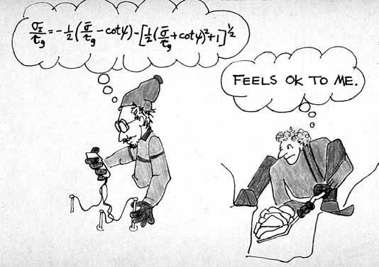
2.1 Snow nerd and the bro 21
2.2 Profiles 22
2.2a Full profile
2.2b Test profile
2.2c Fracture line
2.3 Possible locations for a fracture profile 23
2.4 Targeted site for a snow profile 24
2.5 Layered nature of the seasonal snow cover 25
2.6 Snow crystals 27
2.6a Partially rimed new snow
2.6b Near surface facets
2.6c Rounded grains
2.6d Clustered melt forms
2.6e Facets
2.6f Depth hoar
2.7 Field notes from a test profile 28
2.8 Hand drawn full snow profile on a template ................... 29
2.9 Two methods to record field notes from a full profile 30
2.10 Shovel Shear 33
2.11 Stepping onto a rutschblock 34
2.12 Rutschblock schematic 34
2.13 Field notebook method for recording RB results 35
2.14 Compression Test ............................................................. 36
2.15 ECT ..................................................................................... 38
2.16 PST schematic 40
2.17 PST photo 40
2.18 Slope cut 41
2.19 Hand shear test 43
2.20 Ski pole penetrometer 43
2.21 Shovel tilt test ................................................................... 44
2.22 Ram schematic .................................................................. 45
2.23 Ram sample field book page 46
2.24 Ram calculation worksheet 46
2.25 Ram graph 47
2.26 Shear frame 48
CHAPTER 3
3.1 Slab avalanche .................................................................... 49
3.2 Measuring slope angle 50
3.3 Avalanche types 51
3.3a Soft slab crown
3.3b Wet debris
3.3c Hard slab debris
3.3d Loose snow avalanche/point release
3.4 Slab triggered by loose snow ........................................... 54 3.5 Remote triggered avalanche 55 3.6 Slab avalanche 58 3.7 Trees damaged by avalanche 58
APPENDIX D
D.1 Remote weather station .................................................... 71
D.2 Utah DOT study site ........................................................... 72
D.3 Study plot 73
D.4 Weather station coated in rime 73
D.5 Automated weather instrumentation 74
APPENDIX F
F.1 Snow crystals ....................................................................... 77
F.1a Precipitation particle F.1b Depth hoar
F.2 Snow crystals 78
F.2a Array of precipitation particles F.2b Rounded snow grains
F.3 Large soft slab on facets 80 F.4 Surface hoar ........................................................................ 82 F.5 Large grain surface hoar 85
APPENDIX G
G.1 Vegetation damage 86
G.2 Widespread avalanche activity 87
G.3 North American Public Danger Scale.............................. 88
G.4 Avalanche strikes a road ................................................... 89
G.5 Avalanche hazard scale for transportation corridors 89 G.6 Likelihood of avalanches 90
APPENDIX I
I.2 Snow profile templates 106
I.5 Nomogram ......................................................................... 110
7
ACKNOWLEDGMENTS
The observations and recording practices listed in this document were developed or implemented by the people working with ava lanches in the United States, starting just after World War II and continuing until today. This work was not developed in isolation. Rather it evolved from the fruitful collaboration with scientists and practitioners in many parts of the world, including Canada, Europe, Scandinavia, and Asia. Whenever possible, the contents of this book attempt to align with international standards and standards set by other relevant disciplines.
The seed of the first edition of Snow, Weather, and Avalanches: Observation Guidelines for Avalanche Programs in the United States (SWAG) was a publication of the Canadian Avalanche Association (CAA) entitled Observational Guidelines and Recording Standards for Weather, Snowpack, and Avalanches (OGRS). The CAA devoted a tremendous amount of time and money to creating and maintain ing the OGRS document, which became a symbol of professional practice in North America. With the CAA’s support, the American Avalanche Association (A3) and the USDA Forest Service National Avalanche Center (NAC) provided structure and funding to collect practices from the United States and produce the first edition of SWAG in 2004. The document was revised in 2010, and again in 2016.
The list of people that have contributed to the evolution of SWAG is getting quite long. The committee that produced the first version included Karl Birkeland, Kelly Elder, Greg Johnson, Chris Landry, Ian McCammon, Mark Moore, Don Sharaf, Craig Sterbenz, Bruce Tremper, Knox Williams, and myself. The original effort could not have been completed without the support of Clair Israelson, Janet Kellam, and Doug Abromeit. Dale Atkins and Brian Lazar joined the committee for the second edition, and Mark Staples and Doug Krause (as editor) for the third. For this edition, Simon Trautman and Wendy Wagner joined the team. In addition to all these people, I want to acknowledge the contribution of the following people to this growing body of work: Pat Ahern, Jon Andrews, Don Bachman, Ned Bair, Hal Boyne, Cam Campbell, Doug Chabot, Steve Conger, Mike Cooperstein, Jeff Deems, Nolan Doesken, Pascal Haegeli, Dave Hamre, Dave Gauthier, Bill Glude, Charles Fierz, Liam Fitzgerald, Bruce Jamieson, Ron Johnson, Chris Joosen, Dan Judd, Art Judson, Tom Kimbrough, Mark Kozak, Spencer Logan, Bill Lerch, Tom Leonard, Chris Lundy, Hans-Peter Marshall, Tom McKee, Art Mears, Peter Martinelli Jr., Rod Newcomb, Erich Peitzsch, Ron Perla, Nancy Pfeiffer, Scott Savage, Ron Simenhois, Grant Statham, Ian Tomm, and Joyce VanDeWater. Instructors and students from many venues have offered constructive criticism, which has improved the clarity and focus of the text. Many people provided images for this publication and they are listed with their contributions. Our community continues to contribute to and improve this work. I apologize to anyone that I forgot.
Lastly, I would like to thank Jayne Nolan, Emma Walker, and McKenzie Long for their work on this version of SWAG, and the current members of the American Avalanche Association’s Observation Standards Committee for their dedication, patience, and the hard work they put into revising this document for the 4th edition.
Ethan Greene
Observations and Standards Committee, Chair
Colorado Avalanche Information Center
Leadville, Colorado
August 2022
8
INTRODUCTION
This document contains a set of guidelines for observing and recording snow, weather, and avalanche phenomena. These guidelines were prepared for avalanche forecasting operations, but can be applied to other programs as well. The guidelines are presented as a resource of common methods and are intended to promote efficient and fruitful communication among pro fessional operations and between research and operational communities.
The observations presented in this manual were selected to sup port active avalanche forecasting programs. Observing these parameters will help avalanche forecasters make informed and consistent decisions, provide current and accurate information, and document methods and rationale for operational decisions. Recording these parameters will assist program managers in documenting and analyzing unusual events, applying pattern recognition and statistical forecasting methods, and assisting research into snow and avalanche phenomena. In addition, there is often little snow and weather data collected in mountainous areas, and data collected by avalanche forecasting programs can be used in climatological and mountain systems research. Our hope is that this manual will help forecasters carefully choose the observations that support their programs, and that those obser vations will generate consistent, high-quality data sets.
It is unlikely that any one operation will make all of the obser vations outlined within this document. Individual program managers should select a set of parameters that their staff can observe routinely. Programs with specialized needs may have to look elsewhere for information on additional observations. A set of references is listed in Appendix A as a starting point.
STRUCTURE OF THIS MANUAL
This manual is divided into three chapters and nine appendices. Within each chapter, methods for composing an observational
scheme are presented first. A standard observation is presented next, and the remainder of each chapter is devoted to describing detailed methods for observing and recording a particular phe nomenon. The appendices provide additional information with out distracting from the main topics within the manual.
UNITS
The avalanche community within the United States typically uses a combination of English and International (SI) unit systems. In this document we have attempted to adhere to the SI system whenever possible. In the United States, personnel of avalanche operations and users of their products may not be familiar with all SI units. Individual programs should choose a unit system that suits their particular application. A recommended system of units, an alternative system of English units, and methods for converting values between the two systems are presented in Appendix B. The most noticeable deviation from the SI system is the unit for elevation. In North America most topographic maps use feet as the unit for elevation. Therefore the recommended unit for elevation remains the foot. Throughout the document the recommended unit appears in the text with the common alterna tive unit adjacent in parentheses. Long-term data records should be stored in the recommended system of units in Appendix B. Data records submitted to a central database are assumed to be in the recommended system unless otherwise stated in the accompanying metadata file (see Appendix C).
DATA CODES AND SYMBOLS
Symbols and data codes for many of the observations in this document appear in tables within each section. The use of these codes will save space in field books and on log sheets. Many of the codes in Chapter 1 follow conventions from the meteorolog ical community. The codes in Chapters 2 and 3 were chosen to conform to common methods in the avalanche community and to promote efficient communication.
9
Sections marked with describe parameters included in a standard observation.
MANUAL SNOW AND WEATHER OBSERVATIONS
1.1 INTRODUCTION
Manual observations of snow and weather conditions are an important part of an avalanche forecasting operation. This chapter describes methods for making and recording these observations. Section 1.2 describes observation objectives. Section 1.3 outlines the recommended standard morning snow and weather observation. Sections 1.4 through 1.6 give import ant background information for planning and implementing observational schemes, Sections 1.7 and 1.8 discuss field obser vations, and Sections 1.9 through 1.27 describe how to observe and record individual parameters.
1.2 OBJECTIVES
Snow and weather observations represent a series of meteo rological and snow surface measurements taken at a properly instrumented study plot or in the field (refer to Appendix D). Observational data taken at regular intervals provide the basis for recognizing changes in stability of the snow cover and for reporting weather conditions to a meteorological office or regional avalanche center.
Sustained long-term data sets of snow and weather obser vations can be used to improve avalanche hazard forecasts by statistical and numerical techniques. These data sets also serve to increase climatic knowledge of an area. Observations should be complete, accurate, recorded in a uniform manner, and made routinely. Following an established protocol increases the consis tency in the data record, reduces error, and increases the poten tial for useful interpretation of the data.
day. Listed below is a set of suggested fields to observe and record, and a brief explanation of each. Detailed information on each of these parameters is available in the sections that follow. Sections that are marked with a contain information on the parame ters listed below. An example record sheet appears in Figure 1.2.
1. Observation Location — Record the location of the observation site or nearest prominent topographic land mark (mountain, pass, drainage, avalanche path, etc.), political landmark (town, road mile, etc.), or geographic coordinates (latitude/longitude or UTM). If the measure ments are made at an established study site, record the site name or number.
2. Elevation (ASL) — Record the elevation of the observa tion site in feet (meters) above sea level.
3. Date — Record the date on which the observation is being made (YYYYMMDD).
4. Time — Record the standard local time on the 24-hour clock (0000–2359) at which the observation began.
5. Observer — Record the name or names of the personnel that made the observation.
6. Sky Conditions — Record the sky conditions as Clear, Few, Scattered, Broken, Overcast, or Obscured (Section 1.12).
7. Current Precipitation — Record the precipitation type and rate using the scale and data codes in Section 1.13.
8. Air Temperature — Record the 24-hour maximum, min imum, and current air temperature to the nearest 0.5 °C (or whole °F) (Section 1.14).
9. Snow Temperature 20 cm (or 8 in) — Record the snow temperature 20 cm (or 8 in) below the snow surface (Section 1.17).
10. Surface Penetration — Record the surface penetration to the nearest whole centimeter (or 0.5 inch) as described in Section 1.18.
11. Total Snow Depth — Record the total depth of snow on the ground to the nearest whole centimeter (or 0.5 inch) (Section 1.20).
12. 24-hour New Snow Depth — Record the depth of the snow that accumulated during the previous 24 hours to the nearest whole centimeter (or 0.5 inch) (Section 1.21).
13. 24-hour New Snow Water Equivalent — Record the water equivalent of the snow that accumulated during the previous 24-hours to the nearest 0.1 mm (or 0.01 inch) (Section 1.22).
14. 24-hour Liquid Precipitation — Record the depth of the liquid precipitation that accumulated during the previous 24 hours to the nearest 0.1 mm (or 0.01 inch) (Section 1.24).
1.3 STANDARD MORNING SNOW AND WEATHER OBSERVATION
Operations that include an avalanche forecasting program typically observe and record a set of weather and snow parameters daily. These observations should be made at about the same time each day and between 4 am and 10 am local standard time. Many oper ations will need to observe these parameters more than once per
15. Wind Direction — Observe the wind for at least two minutes and record the average wind direction or use an automated measurement. Record wind direction relative to true north as N, NE, E, SE, S, SW, W, or NW. If an automated measure ment is used, record to the nearest 10 degrees (Section 1.26).
16. Wind Speed — Observe the wind for at least two minutes and record the average wind speed using the indicators in Section 1.26, or use an automated measurement.
10
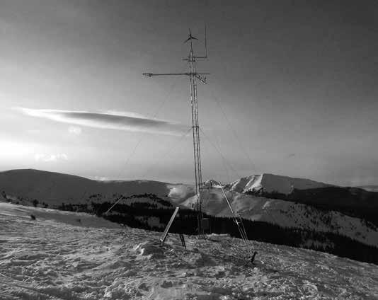
FIGURE 1.1 Alpine weather station in the Colorado Rocky Mountains. ! Kelly Elder
17. Maximum Wind Gust — Observe the wind for at least two minutes and record the speed of the strongest wind gust, or use an automated measurement. For an auto mated measurement record the time that the wind gust occurred (Section 1.26).
1.4 MANUAL VS. AUTOMATED OBSERVATIONS
Observation networks for avalanche forecasting programs usually involve at least one set of manual observations and one or more automated weather stations (Figure 1.1). Manual observations can be used to maintain a long-term record and observe and record data not amenable to sensing by automated systems. Automated observations provide unattended contin uous weather (and some snowpack) information about a cer tain region or regions within a forecast or ski area. Automated weather stations can be co-located at study sites where manual weather observations and/or snowpack observations are col lected. Programs that maintain a study plot should use data from automated weather stations to augment and not replace manual observations. The following chapter discusses how to make and record manual observations. Details regarding automated snow and weather observations appear in Appendix E.
1.5 TIME PERIODS FOR MANUAL SNOW AND WEATHER OBSERVATIONS
Observations made daily at a specific time are called standard observations. Manual observations are typically carried out in 24-hour, 12-hour, or 6-hour intervals. Data collected at 6-hour intervals beginning at 0000 hours Greenwich Mean Time (also termed Coordinated Universal Time (UTC) or Zulu time (Z)) will conform to climatic data sets. Avalanche forecasting opera tions typically make two standard observations each day at 0700 and 1600 hours standard local time, when a 12-hour interval is not possible. The type of operation and availability of observ ers may drive different observation frequencies and times. Operations should record the time of the observation in local standard time, even in regions that observe Daylight Savings Time. If observers choose to make only one standard observa tion each day, it is best to do it at the same time each morning. Observations taken between the standard times are referred to as interval observations. They are taken when the snow stabil ity is changing rapidly, such as during a heavy snowfall. Interval observations may contain a few selected observations or a com plete set of observations.
Observations taken at irregular times are referred to as inter mittent observations. They are appropriate for sites that are vis ited infrequently; visits will typically be more than 24 hours apart and need not be regular (i.e. in a heli-ski operation). Intermittent observations may contain a few selected observations or a com plete set of observations. In highway operations, intermittent observations often include shoot or storm observations to coin cide with the timing of avalanche mitigation or the start and end of particular storm cycles (see Figure 1.2 for sample of field book entry).
It is common for avalanche forecasting operations to col lect information for an individual storm event. Observations of snowfall, temperature changes, wind direction and speed, and avalanche activity can be observed for a particular storm unit. A storm unit is typically a qualitative increment based on
precipitation rates or meteorological events. Operations that choose to use a storm unit may also find it useful to develop a quantitative storm unit definition.
1.6 EQUIPMENT FOR MANUAL STANDARD OBSERVATIONS
A snow and weather study plot usually contains the following equipment:
• Instrument shelter for housing thermometers (height adjustable)
• Maximum thermometer
• Minimum thermometer
• One or more snow boards with 1 m (~3 ft) rods and base plate with minimum dimensions of 40 cm x 40 cm (~15 in) and appropriate labels (Figure 1.3)
• Snow stake, depth marker (graduated in cm (in))
• Ruler (graduated in cm (in))
• Snow sampling tube and weighing scale (graduated in grams or water equivalent), or precipitation gauge
• Large putty knife or plate for cutting snow samples
• Field book and pencil (water resistant paper)
The following additional equipment is useful:
• Hygrothermograph located in an instrument shelter (Figure 1.3)
• Recording precipitation gauge or rain gauge (Figure 1.4)
• Additional snow boards
• First section of a Ram penetrometer
• Barograph (in the office) or barometer/altimeter
• Anemometer at a separate wind station with radio or cable link to a recording instrument (Figure D.4)
• Box (shelter) for the equipment
• Small broom
• Snow shovel
In some cases the weather sensors listed above have been linked to data loggers where, in most instances, comparable data may be obtained (see Appendix E). However, a broken wire or power outage may render automated data useless, so manual observa tions are still preferred as a baseline.
1.7 FIELD BOOK NOTES
There are many good and different methods for taking field notes. Following these general practices will ensure that quality data are collected.
• Do not leave blanks. If a value was not observed, record N/O for not observed or place a dash (-) in the cell of a standard form where a particular observation is missing or never observed.
• Only write “0” when the reading is zero, for example, when no new snow has accumulated on the new snow board.
• Only record values that are actually observed.
1.8 FIELD WEATHER OBSERVATIONS
Heli-ski guiding, ski touring and similar operations often observe general weather conditions in the field. These obser vations may serve as an interval measurement, accompany a snow profile, or serve to document conditions across a portion of their operational area. The records should describe some of
MANUAL SNOW AND WEATHER OBSERVATIONS 11
MANUAL SNOW AND WEATHER OBSERVATIONS
the parameters listed in this section, but field reports should be made as a series of comments so as not to be confused with observations taken at a fixed weather station. Maximum and minimum temperatures cannot be observed, but a range in present temperatures can be reported. Field observations should specify the elevation range and the time, or time range, from where the observations were taken. Common field obser vations typically include: time, location, elevation, sky cover, wind speed and direction, air temperature and precipitation type and rate. Field weather observations that are estimates and not measurements should be recorded with a tilde (~) to denote that the value is approximate.
1.9 LOCATION
Record the location and elevation, or study plot name, at the top of the record book page.
1.10 DATE
Record the year, month and day. Avoid spaces, commas etc.; i.e. December 5, 2022, is noted as 20221205 (YYYYMMDD). This representation of the date is conducive to automated sorting routines.
1.11 TIME
Record the time of observation using a 24-hour clock (avoid spaces, colons etc.) (i.e. 5:10 p.m. is noted as 1710). Use local standard time (i.e. Pacific, Mountain, etc. as appropriate). Operations that overlap time zones should standardize to one time.
1.12 SKY CONDITION
Classify the amount of cloud cover and record it using the defini tions in Table 1.1. Observers may select a separate data code for each cloud layer or one code for the total cloud cover.
TABLE 1.1 Sky Condition
Valley Fog/Cloud
Where valley fog or valley cloud exists below the observation site, estimate the elevation of the top and bottom of the fog layer in feet (meters) above sea level. Give the elevation to the nearest 100 ft (or 50 m). Data code: VF.
Example: Clear sky with valley fog from 7,500 to 9,000 ft is coded as CLR VF 7500-9000.
Thin Cloud
The amount of cloud, not the opacity, is the primary classifica tion criterion. Thin cloud has minimal opacity, such that the disk of the sun would still be clearly visible through the clouds if they were between the observer and the sun, and shadows would still be cast on the ground. When the sky condition features a thin scattered, broken or overcast cloud layer then precede the sym bol with a dash.
Example: A sky completely covered with thin clouds is coded as -OVC.
1.13 PRECIPITATION TYPE, RATE, AND INTENSITY
The amount of snow, rain, or water equivalent that accumulates during a time period will help forecasters determine the rate and magnitude of the load increase on the snowpack. In this document, Precipitation Rate refers to an estimate of the snow or rain rate. Precipitation Intensity is a measurement of water equivalent per hour.
Procedure
Precipitation Type
Note the type of precipitation at the time of observation and record using the codes in Table 1.2.
CLASS SYMBOL DATA CODE DEFINITION
Clear CLR No clouds
Few FEW Few clouds: up to 2/8 of the sky is covered with clouds
Scattered SCT Partially cloudy: 3/8 to 4/8 of the sky is covered with clouds
Broken BKN
Cloudy: more than half but not all of the sky is covered with clouds (more than 4/8 but less than 8/8 cover)
Overcast OVC Overcast: the sky is completely covered (8/8 cover)
Obscured X A surface-based layer (i.e. fog) or a non-cloud layer prevents observer from seeing the sky
12
DATA CODE DESCRIPTION
NO No Precipitation
RA Rain SN Snow
RS Mixed Rain and Snow
GR Graupel and Hail
ZR Freezing Rain
Precipitation Rate
Use the descriptors listed in Table 1.3 to assess the precipitation rate at the time of observation. Record the estimated rate with the appropriate data code in Table 1.3.
Precipitation Intensity
Use measurements of rain or the water equivalent of snow to calculate the precipitation intensity with the following equation:
PI ( )mm water equivalent of precipitation (mm) hr duration of measurement period (hr) =
Record the results with the data code PI and the measured value in millimeters (inches) of water.
Note: PI values are assumed to be in millimeters, and duration is assumed to be one hour. Use the symbol '' to signify when inches are used.
TABLE 1.3 Precipitation Rate
Example: A precipitation intensity of one half inch per hour would be coded as PI 0.5''.
1.14 AIR TEMPERATURE
Temperature is measured in degrees Celsius (abbreviated °C) or degrees Fahrenheit (°F). The standard air temperature should be observed in a shaded location with the thermometer 1.5 m above the ground or snow surface. At a study site, thermometers should be housed in an instrument shelter and the lower edge of the screen should be 1.2 to 1.4 meters above the ground or snow surface (Figure 1.3 ).
Procedure
1. Read the maximum thermometer immediately after opening the instrument shelter.
2. Read the present temperature from the minimum ther mometer, and read the minimum temperature from the minimum thermometer last.
3. Read temperature trend and temperature from the thermograph.
At the end of the temperature observation:
4. Remove any snow that might have drifted into or accu mulated on top of the screen.
5. Reset the thermometers after the standard observations (refer to Appendix D).
6. If the instrument shelter is fitted with a height adjustment mechanism, ensure that the screen base is in the range of 1.2 to 1.4 m above the snow surface. (Note: In heavy snow
DATA CODE DESCRIPTION RATE
Snowfall Rate (this table provides examples; any appropriate rate may be specified)
S-1
Very light snowfall
S1 Light snowfall
S2 Moderate snowfall
S5
S10
Rainfall Rate
Heavy snowfall
Very heavy snowfall
RV Very light rain
RL Light rain
RM Moderate rain
RH Heavy rain
Snow accumulates at a rate of a trace to about 0.5 cm (~ 0.25 in) per hour
Snow accumulates at a rate of about 1 cm (~ 0.5 in) per hour
Snow accumulates at a rate of about 2 cm (a little less than 1 in) per hour
Snow accumulates at a rate of about 5 cm (~ 2 in) per hour
Snow accumulates at a rate of about 10 cm (~ 4 in) per hour
Rain produces no accumulation, regardless of duration
Rain accumulates at a rate up to 2.5 mm (0.1 in) of water per hour
Rain accumulates at a rate between 2.6 to 7.5 mm (0.1 to 0.3 in) of water per hour
Rain accumulates at a rate of 7.5 mm (0.3 in) of water per hour or more
MANUAL SNOW AND WEATHER OBSERVATIONS 13
TABLE 1.2
Precipitation Type
climates where daily access of the site is not always possible, the instrument shelter may be mounted on top of a tower to prevent burial. However the height of the screen should be noted in the metadata.)
7. Check that the screen door still faces north if any adjust ments are made.
Read all air temperatures from thermometers to the nearest 0.5 °C (or whole °F). If there is snow on the thermometer it should be brushed off prior to reading the instrument and noted in the comment section.
1.14.1 AIR TEMPERATURE TREND
If available, read the air temperature from the thermograph and record to the nearest whole degree. Use an arrow symbol or data code to record the temperature trend shown on the thermograph trace over the preceding three hours.
Note: Table 1.4 assumes the use of the Celsius temperature scale. Operations that use the Fahrenheit temperature scale should use a threshold of 10 degrees (rather than 5 degrees) for rapid tempera ture changes.
Time, Type (Std, Int) 0530, S
I 0530, S 1630, S 0530, S 1630, S Sky BKN OVE
OVC OVC
Precip Type/Rate NO SN, S-1 SN, S1 SN, S3 RA, RL NO Max Temp (°C) -2.5 -3 -3 -1.5 1 0 Min Temp (°C) -7 -6 -4.5 -4 -4 -11 Present Temp (°C) -6.5 -3 -4 -1.5 0 -10 Thermograph (°C) -7 -3 -4 -1 0 -10 Thermograph Trend S R S R S FR 20 cm Snow Temp (°C) -10 -6 -5 -4 -4 -6 Relative Humidity (%) 78 86 96 98 100 67 Interval (cm) HIN 0 T 10 12 4 0 Standard (cm) H2D 0 T 10 12 15 0 New (cm) HN24 0 T 10 12 15 14 Storm (cm), C=cleared HST 0 T 10 20 21 19,C Snow depth (cm) HS 223 222 231 239 241 239 New water (g) 0 N/O 33.6 42 67 0 New water (mm) 0 N/O 8 10 16 0 Density (kg/m³) N/O 80 83 106 0 Rain gauge (mm) 3 Precip gauge (mm) 60 60 67 77 82 82 Foot Pen (cm) 35 35 45 50 50 45 Ram Pen (cm) 40 39 47 55 55 48 Surface Form / Size (mm) N/O PP/1.0 PP/1.0 PP/1.5 MF/0.5 DF/0.5 Wind Speed / Direction L, E Calm M, SE L, S L, SW M, E Blowing Snow Extent / Dir U None L, SE M, S Prev None Barometric Pressure (mb) 852 847 817 813 833 843 Pressure Trend S F FR F RR RR Comments
FIGURE 1.2 An example standard observation record sheet.
14
MANUAL SNOW AND WEATHER OBSERVATIONS
SITE #4,
IM IM DS DS KE KE
LOCATION NEVER SUMMER
8,300' Observer
Date 20220210 20220211 20220212 20220213 20220214 20220215
1730,
OVC
CLR
SYMBOL DATA CODE DESCRIPTION
RR
Temperature rising rapidly (> 5-degree increase in past 3 hours)
R Temperature rising (1- to 5-degree increase in past 3 hours)
S Temperature steady (< 1-degree change in past 3 hours)
F Temperature falling (1- to 5-degree decrease in past 3 hours)
FR Temperature falling rapidly (> 5-degree decrease in past 3 hours)
1.15 RELATIVE HUMIDITY (RH)
Read the relative humidity to the nearest one percent (1%) from the hygrograph or weather station output.
The accuracy of relative humidity measurements decreases at low temperatures. Furthermore, the accuracy of any mechanical hygrograph is unlikely to be better than five percent (5%) but trends may be important, especially at high RH values. Refer to Appendix D for information on exposure issues and relative humidity measurements.
Depending on location, humidity measurements may be more relevant from mid-slope or upper-elevation sites than from valleybottom sites.
Hygrographs should be calibrated at the beginning of each season, mid-season, and after every time the instrument is moved. Calibration is most important when data from multiple instruments are compared with each other. The simplest cali bration method is to make a relative humidity measurement near the instrument shelter with a psychrometer (aspirated or sling). Calibration should be done midday or at a time when the air temperature is relatively stable. Psychrometer measure ments are easier to perform when the air temperature is near or above freezing.
1.16 BAROMETRIC PRESSURE AT STATION
The SI unit for pressure is the pascal (Pa). For reporting weather observations, barometric pressure should be recorded in millibars (1 mb = 1 hPa = 100 Pa, see Appendix B). The recommended English unit for barometric pressure is inches of mercury (inHg). Conversions from other commonly used pressure units to millibars and inches of mercury are listed in Appendix B.
1.16.1 PRESSURE TREND
Use an arrow symbol to record the pressure trend as indicated by the change of pressure in the three hours preceding the
SYMBOL DATA CODE DESCRIPTION
RR Pressure rising rapidly (>2 mb rise per hour)
R Pressure rising (<2 mb rise per hour)
S Pressure steady (<1 mb change in 3 hours)
F Pressure falling (<2 mb fall per hour)
FR Pressure falling rapidly (>2 mb fall per hour)
observation. Record the change in barometric pressure in the past three hours.
1.17 20 CM SNOW TEMPERATURE
(T20)
Dig into the snow deep enough to allow access to an area 20 cm (or 8 in) below the surface. Cut a shaded wall of the pit smooth and vertical. Shade the snow surface above the area where the sensor will rest in the snow. Cool the thermometer in the snow at the same height, but a different location than where the mea surement will be taken. Insert the thermometer horizontally 20 cm (or 8 in) below the snow surface and allow it to adjust to the temperature of the snowpack. Once the sensor has reached equilibrium, read the thermometer while the sensor is still in the snow.
Record snow temperature to the nearest degree or fraction of a degree based on the accuracy and precision of the thermometer.
1.18 SURFACE PENETRABILITY
(P)
An indication of the snowpack’s ability to support a given load and a relative measure of snow available for wind transport can be gained from surface penetrability measurements. There are several common methods for examining surface penetration. Ram penetration is the preferred method of observation because it produces more consistent results than ski or foot penetration. When performing foot or ski penetration on an incline, average the uphill and downhill depths of the track.
Procedure
Ram Penetration (PR)
Let the first section of a standard Ram Penetrometer (cone diam eter 40 mm, apex angle 60° and mass 1 kg) penetrate the snow slowly under its own weight by holding it vertically with the tip touching the snow surface and dropping it. Read the depth of penetration in centimeters.
Foot Penetration (PF)
Step into undisturbed snow and gently put full body weight on one foot. Measure the depth of the footprint to the nearest cen timeter (or whole inch) from 0 to 5 cm and thereafter, to the nearest increment of 5 cm (or 2 in).
MANUAL SNOW AND WEATHER OBSERVATIONS 15
TABLE 1.4 Temperature
Trend
TABLE 1.5 Pressure Trend
The footprint depth varies between observers. It is recom mended that all observers working on the same program com pare their foot penetration. Observers who consistently produce penetrations more than 10 cm (or 4 in) above or below the aver age should not record foot penetrations.
Ski Penetration (PS)
Step into undisturbed snow and gently put full body weight on one ski. Measure the depth of the ski track from its centerline to the nearest centimeter (or whole inch) from 0 to 5 cm and there after, to the nearest increment of 5 cm (or 2 in).
Ski penetration is sensitive to the weight of the observer and the surface area of the ski.
1.19 FORM (F) AND SIZE (E) OF SURFACE SNOW
Record the form and size in millimeters of snow grains at the surface using the International Classification for Seasonal Snow on the Ground, (Fierz and others, 2009) basic classification (Table 1.6).
Experienced observers may use the subclasses (Table 1.7) to dis criminate between various types of surface deposits and crusts (refer to Appendix F for more detailed information about grain forms).
1.20 HEIGHT OF SNOWPACK (HS)
The height of the snowpack should be measured at a geographi cally representative site, preferably within 100 meters (or 300 ft) of the weather study plot. A white stake graduated in centime ters (inches) should be placed at the site. It is best to preserve an area with a radius of about 3 m (or 10 ft) around the snow stake for measurements. Ideally the snow in this area is not disturbed during the winter. Leave naturally forming settlement cones and depressions in place and try not to walk through the area.
Procedure
From a distance of about 3 m (or 10 ft) look across the snow sur face at the snow stake. Observe the average snow depth between your position and the stake to the nearest centimeter (or 0.5 inch). Try not to disturb the snow around the stake during the course of a winter season. HS values are measured vertically (i.e. line of plumb).
1.21 HEIGHT OF NEW SNOW (HN24)
The new snow measurement in the standard morning observa tion uses a 24-hour interval. Many operations will find it useful to observe snowfall on more than one interval. However, the 24-hour interval snow board should only be used for 24-hour observations. Additional snow boards should be added for addi tional observations as necessary. It is highly recommended that both 24-hour and Storm intervals be observed by operations that maintain a study plot. Other commonly used intervals appear in the Snow Board Naming Convention Section 1.21.1.
New snow measurements should be made on a snow board (Figure 1.3). The base plate should have minimum dimensions of 40 cm x 40 cm (or 15 in x 15 in), with an attached rod of 1 m (or 3 ft) in length. Larger boards (60 cm x 60 cm) provide more room to make measurements. The base plate and rod should be painted white to reduce the effects of solar heating.
TABLE 1.6 Basic Classification of Snow on the Ground
SYMBOL DESCRIPTION DATA CODE + Precipitation Particles (New Snow) PP
Machine Made Snow MM / Decomposing and Frag mented Particles DF
Grains
Depth Hoar DH
Ice Formations IF
Note for Table 1.6: Modifications to Fierz and others, 2009: A subscript “r” modifier is used to denote rimed grains in the Decomposing and Fragmented Particles (DF) major class and the Precipitation Particles (PP) major class and its subclasses except for gp, hl, ip, rm (Example: PP-r). Subclasses for surface hoar are listed in Appendix F.
TABLE 1.7 Surface Deposits and Crusts Subclasses
SYMBOL CLASSIFICATION DATA CODE r Rime PPrm
Rain crust IFrc Sun crust, Firnspiegel IFsc y Wind packed RGwp Oh Melt freeze crust MFcr
Procedure
Use a ruler graduated in centimeters (or inches) to measure the depth of snow accumulated on the snow board. Take measure ments in several spots on the board. Calculate the average of the measurements and record to the nearest cm (in). Record “T” (signifying a trace) when the depth is less than 1 cm (or 0.5 in), or when snow fell but did not accumulate. If there is no new snow, record zero. Do not consider surface hoar on the boards as snowfall; clear off hoar layer after observation. If both rain and snow fell, it should be noted in the remarks.
The sample on the snow board can also be used to measure the water equivalent of new snow (Section 1.22). Once the observa tions are complete, redeposit the snow in the depression left by the snow board, adding additional snow if necessary to reposi tion the board level with the surrounding snow surface.
If the snow board was not level, the measurement should be made normal to the surface of the board.
16
MANUAL SNOW AND WEATHER OBSERVATIONS
∧
∨
▄
⌾
� Rounded
(monocrystalline) RG � Faceted Crystals FC
Surface Hoar SH ○ Melt Forms MF
1.21.1 SNOW BOARD NAMING CONVENTIONS
The following conventions can be used to identify snow boards used for different interval measurements.
HN24—24-hour Board: The HN24 board is used to measure snow that has been deposited over a 24-hour period. It is cleared at the end of the morning standard observation.
HST—Storm Board: Storm snowfall is the depth of snow that has accumulated since the beginning of a storm period. The storm board is cleared at the end of a standard observation prior to the next storm and after useful settlement observations have been obtained. The symbol “c” is appended to the recorded data when the storm board is cleared.
H2D—Twice-a-Day Board: An H2D board is used when stan dard observations are made twice a day. In this case both the HN24 and H2D boards should be cleared in the morning and then the H2D board is cleared again in the afternoon.
HSB—Shoot Board: The shoot board holds the snow accumu lated since the last time avalanches were shot with explosives. The symbol “c” is appended to the recorded data when the shoot board is cleared.
HIN—Interval Board: An interval board is used to measure the accumulated snow in periods shorter than the time between standard observations. The interval board is cleared at the end of every observation.
HIT—Intermittent Board: Snow boards may be used at sites that are visited on an occasional basis. Snow that accumulates on the board may result from more than one storm. The intermit tent snow board is cleared at the end of each observation.
1.22 WATER EQUIVALENT OF NEW SNOW
(HN24W)
The water equivalent is the depth of the layer of water that would form if the snow on the board melted. It is equal to the amount of liquid precipitation. The standard morning observation includes the water equivalent of the new snow on a 24-hour interval. The same snow board used for a 24-hour or other interval measure ment should be used to calculate the water equivalent. There are several suitable methods for making this measurement. Three different methods are described in the following section.
Procedure
Use one of the following methods to calculate the water equiv alent of the new snow. Record the value to the nearest 0.1 mm (or 0.01 in). Make several measurements and report the average value. Record “T” (signifying a trace) when the snow depth is less than 1 cm (or 0.5 in). If there is no new snow, record a zero. Do not consider surface hoar on the boards as snowfall; clear off hoar layer after observation.
Snow Board Tube and Weighing Scale
1. Cool the measurement tube in the shade prior to making the measurement and tare the empty tube on the scale
2. Hold the tube vertically above the surface of the snow on the snow board
3. Press the tube into the snow at a slow and constant rate until it hits the base plate of the snow board
4. Record the height of the snow sample in the tube
5. Remove the snow next to one side of the tube with a large putty knife or scraper
6. Slide putty knife under the tube and remove the sample from the board
7. Weigh the sample and read the water content from the scale, or use the equation listed below, or the SWE nomogram in Appendix I
MANUAL SNOW AND WEATHER OBSERVATIONS 17
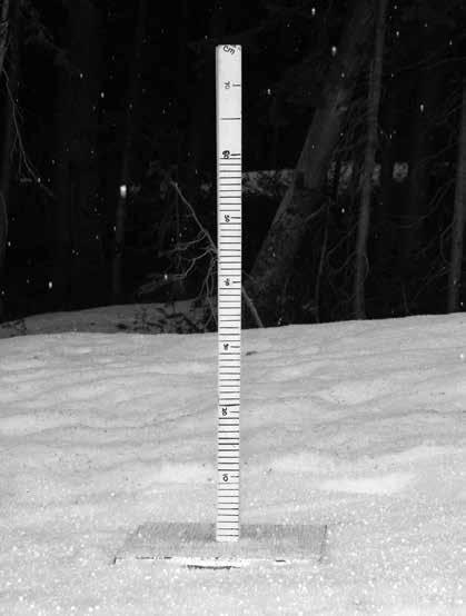
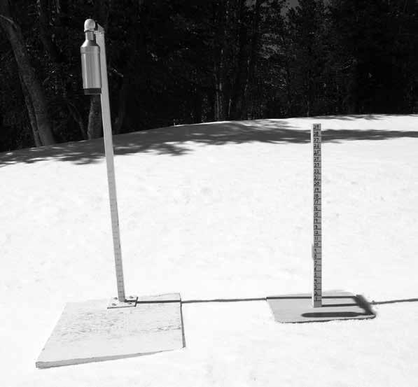
FIGURE 1.3 Left: Snow board graduated in centimeters. Right: Automated snow board and snow board graduated in inches. ! Tom Leonard
8. Repeat and record the average of several measurements to the nearest 0.1 mm (or 0.01 in)
9. Record the measurement by indicating the snow board it was taken from. For example, HN24W is the water equiv alent of the snow on the HN24 board
Melting the Snow Sample
The water equivalent of the new snow can be obtained by melt ing a sample of snow and measuring the resulting amount of melt water. The height of the melt water in mm (in) is the water equiv alent of the sample. When using this method, the base area of the snow sample and the melted sample must remain the same.

Indirect Method
operations to discuss snow density in percent water content per volume. Calculations of both quantities are described below. Data records of snow density should be recorded in units of kg/m3. The Greek symbol ρ (rho) is used to represent density.
Calculating Density
Divide the mass (g) of new snow by the sample volume (cm3) and multiply by 1000 to express the result in kilograms per cubic meter (kg/m3). Record as a whole number (i.e. 120 kg/m3).
For measurements from standard observations:
ρ( )kg mass of snow sample (g) m3 sample volume (cm3) = x 1000 ρ( )kg HN24W (mm) m3 H2D (cm) = x 100
HN24W (mm) mass of snow sample (g) area of sample tube (cm2) =
x 10
The water equivalent of snow can also be obtained by weighing a snow sample of known cross-sectional area. Water equivalent is calculated by using the following equation: This method is commonly used by avalanche operations because of its ease (Note: 1 cm3 of water has a mass of 1 g). The expanded equation is in Appendix B, Section B.5.

1.23 DENSITY OF NEW SNOW (ρ)
Density is a measure of mass per unit volume; density is expressed in SI units of kg/m3. It is also common for avalanche
The density of a snow sample is often communicated as a dimensionless ratio or percent. Calculate this ratio by divid ing the height of the water in a snow layer by the height of the snow layer and then multiply by 100 (e.g. 10 cm of snow that contains 1 cm of water has a water content of 10%). This ratio can also be calculated by dividing the density of the snow (kg/ m 3) by the density of water (1000 kg/m3) and multiplying by one hundred. Using the density of water allows for an easy calculation by moving the decimal one space to the left (i.e. 80 kg/m 3 = 8%).
18 MANUAL SNOW AND WEATHER OBSERVATIONS
FIGURE 1.4 Precipitation gauge with Alter shield. ! Tom Leonard
FIGURE 1.5 Evidence of previous blowing snow. ! Kelly Elder
% water water equivalent of snow sample (mm) height of snow sample (mm) =
% water water equivalent of snow sample (mm) height of snow sample (cm) =
% water water equivalent of snow sample (in) height of snow sample (in) =
1.24 RAIN
x 100
x 10
point. Estimates are made without instruments or with handheld instruments, and typically represent wind in a local area rather than at a fixed point.
Procedure
Measured Wind Speed
x 100
There are a variety of commercial rain gauges available. The stan dard rain gauge is made of metal and has an 8-inch (~20 cm) orifice (Figure 1.4). However, good results can be obtained with commercially manufactured 4-inch (~10 cm) diameter plas tic gauges. The gauge should be mounted at the study site (see Appendix D for site guidelines). If a mounted gauge is not avail able, an 8-inch (~20 cm) gauge may be placed on the snow board prior to a rain event.
Procedure
Measure the amount of rain that has accumulated in the rain gauge with the length scale on the gauge or a ruler. Record the amount to the nearest 0.1 mm (or 0.01 in). Empty the gauge at each standard observation.
1.25 ACCUMULATED PRECIPITATION
Accumulated precipitation gauges collect snowfall, rainfall and other forms of precipitation and continuously record their water equivalent. There are a variety of commercial gauges (both man ual and automated) available.
Procedure
Record the amount of precipitation accumulated in the record ing precipitation gauge to the nearest tenth of a millimeter (0.1 mm) or 0.01 of an inch. The amount of precipitation that fell during a single event can be obtained by taking the difference between the present reading and the previous reading.
1.26 WIND
Both estimates and measurements of wind speed and direc tion are useful to observe and record. However, it is import ant to distinguish between the two types of observations. Measurements are made with an instrument located at a fixed
TABLE 1.8 Wind Speed Estimation
CLASS
The SI unit for wind speed is meters per second (miles per hour). Refer to Appendix B for unit conversions.
Measured Maximum Wind Gust
Record the speed and time of occurrence of the maximum wind gust.
Measured Wind Direction
Measured wind direction for standard observations should be rounded to the nearest 10 degrees (i.e. 184 degrees—just beyond south—is coded as 180). Forty-five degrees (northeast) is coded as 050. Archived wind direction data from an automatic weather station can be stored as a three digit number. Wind direction is always given relative to true north.
Estimated Wind Speed
For the standard morning observation, an estimate of the wind speed can be obtained by observing for two minutes. Use the indicators in Table 1.8 to determine the categorical wind speed and the data codes to record average conditions during the observation period.
The indicators used to estimate the wind speed are established by rule of thumb. Observers should develop their own relation ships specific to their area. Wind estimates (speed and direction) should be averaged over a two-minute period prior to the obser vation. Since wind speed classes are determined by an estimate, mi/hr categories can be rounded to the nearest 5 mi/hr.
Estimated Maximum Wind Gust
Estimate the maximum wind speed during the observation period. Record the estimated speed to the nearest 2 m/s (or 5 mi/hr).
Estimated Wind Direction
During a two-minute period, note the direction from which the wind blows. The wind direction can be recorded using the compass directions listed in Table 1.10. Do not record a direc tion when the wind speed is zero (Calm). If no definitive wind direction can be established, record direction as Variable (VAR). Wind direction is always given relative to true north.
DATA CODE KM/H M/S MI/HR TYPICAL INDICATOR
Calm C 0 0 0 No air motion. Smoke rises vertically.
Light L 1-25 1-7 1-16
Light to gentle breeze. Flags and twigs in motion.
Moderate M 26-40 8-11 17-25 Fresh breeze. Small trees sway. Flags stretched. Snow begins to drift.
Strong S 41-60 12-17 26-38
Strong breeze. Whole trees in motion.
Extreme X >60 >17 >38 Gale force or higher.
MANUAL SNOW AND WEATHER OBSERVATIONS 19
FIGURE 1.6
1.27 BLOWING SNOW
Estimate the extent of snow transport (Table 1.9) and note the direction from which the wind blows to the closest octant of the compass (Table 1.10). The observer should also note the location and/or elevation of the wind transport (e.g. valley bottom, study site, ridgetop, peaks, 11,000 ft, 3000 m, etc.). Record wind direc tion as indicated by blowing snow (Figures 1.5 and 1.6).
TABLE 1.9 Extent of Blowing Snow
DATA CODE DESCRIPTION
None No snow transport observed.
Prev Snow transport has occurred since the last observation, but there is no blowing snow at the time of observation.
L Light snow transport.
M Moderate snow transport.
I Intense snow transport.
U Unknown as observation is impossible because of darkness, cloud, or fog.
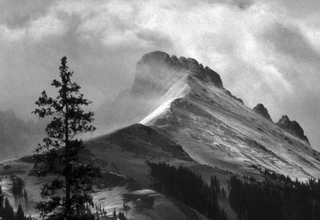
TABLE 1.10 Direction of Wind Relative to True North
DIRECTION N NE E SE S SW W NW DEGREES 0 45 90 135 180 225 270 315
20 MANUAL SNOW AND WEATHER OBSERVATIONS
Evidence of current blowing snow. ! Ethan Greene
SNOWPACK OBSERVATION
2.1 INTRODUCTION
Information on the structure and stability of the snowpack within an area is essential to assessing current and future ava lanche conditions. In certain applications, starting zones may be inaccessible and snowpack properties can be estimated with careful analysis of past and present weather and avalanche events. Snowpack parameters vary in time and space, and observation schemes should address these variations. Snowpack information is generally observed and recorded separately from the snow and weather observations outlined in Chapter 1. However, weather observations can be combined in many ways with snowpack observations (Figure 2.1).
Broad objectives are outlined in Section 2.2. A set of standard parameters to be collected with any snowpack observation fol lows in Section 2.3. Snow profiles and snowpack measurements are described in Sections 2.4 and 2.5. In Section 2.6 methods for observing and recording shear quality are discussed. Section 2.7 presents column and block stability tests; slope cuts are described in Section 2.8; non-standardized tests are described in Section 2.9 and instrumented measures are listed in Section 2.10.
2.2 OBJECTIVES
The primary objective of any observer working in avalanche ter rain is safety. Secondary objectives may include observing and recording the current structure and stability of the snowpack. Other objectives will depend on the type of operation.
Specific measurements and observations will be dependent on the type of operation, but in general the objective is to observe and record the current structure and stability of the snowpack. More specific objectives are listed in the sections that follow.
workers should select snowpack properties (parameter 6) from those listed in this chapter to supply the information needed for their specific application.
1. Date — Record the date on which the observation was made (YYYYMMDD).
2. Time — Record the standard local time on the 24-hour clock (0000–2359) at which the observation began.
3. Observer — Record the name or names of the personnel that made the observation.
4. Site Characteristics
• Observation Location — Record the nearest prominent topographic landmark (mountain, pass, drainage, ava lanche path, etc.), political landmark (town, road mile, etc.), or geographic coordinates (latitude/longitude or UTM and datum). If observing a fracture line profile, note the location within the avalanche path.
• Aspect — Record the direction that the slope faces where the observation was made (i.e. N, NE, E, SE, S, SW, W, NW, or cardinal degrees).
• Elevation — Record the elevation of the observation site (feet or meters).
• Slope Angle — Record the incline of the slope where the observation was made (degrees).
5. Current Weather
• Sky Conditions — Record the sky conditions as Clear, Few, Scattered, Broken, Overcast, or Obscured (Section 1.12).
• Air temperature — Record the current air tempera ture to the nearest 0.5 °C (or whole °F).
• Precipitation Type and Rate — Record the precipita tion type and rate (Section 1.13).
• Wind — Record the wind speed and direction (Section 1.26).
• Surface Penetration — Record the surface penetra tion (Section 1.18).
6. Snowpack Properties — Observe and record the neces sary snowpack properties as described in this chapter.
7. Avalanche Potential — Record one or more of the param eters as applicable to the operation (see Appendix G). Avalanche conditions can be grouped by region, aspect, slope angle range (i.e. 35°–40°), or obvious snow prop erties (such as recently wind loaded or amount of new snow). In this case a separate stability, danger, or hazard rating should be given for each group (Appendix G).
2.3 STANDARD SNOWPACK OBSERVATION
The snowpack parameters observed and the detail of those observations will depend on the particular forecasting problem. This section presents an outline for daily snowpack observations. Parameters 1 through 5 and parameter 7 will be useful for most avalanche forecasting programs. Individual programs and field
A) Snow Stability Forecast — Record the snow stability stated in the morning meeting or current forecast. Observed — Record the snow stability observed at this location.
B) Avalanche Danger Forecast — Record the avalanche danger stated in the current avalanche forecast. Observed — Record the avalanche danger assessed at this location.
21
FIGURE 2.1 There are many different approaches to observing snow pack properties. Illustration by Sue Ferguson
C) Avalanche Hazard
Forecast — Record the avalanche hazard currently stated by the program Observed — Record the avalanche hazard assessed at this location

2.4 SNOW PROFILES
Snow profiles are observed at study plots, study slopes, fracture lines and targeted sites. This section outlines two types of snow profiles: full profiles and test profiles. A full profile is a complete record of snow-cover stratigraphy and characteristics of individ ual layers. A test profile is a record of selected observations.
Full Profiles
Full snow profiles (Figure 2.2) are frequently observed at study plots or study slopes in time series to track changes in the snow pack. They require that all, or most, snowpack variables be mea sured (Section 2.5). Full profiles are time-consuming and not always possible at targeted sites.
Test Profiles
Test profiles (Figure 2.2) are the most common type of snow pro file. There is no fixed rule about the type and amount of infor mation collected in a test profile. Each observer must select, observe, and record the parameters needed by their operation.
These parameters may change in both time and space. Test pro files are commonly observed at targeted sites and fracture lines.
The objectives of observing full profiles are:
1. Identify the layers of the snowpack 2. Identify the hardness and/or density of the layers in the snowpack

3. Identify weak interfaces between layers and to approximate their stability 4. Observe snow temperatures 5. Monitor and confirm changes in snowpack stability 6. Determine the thickness of a potential slab avalanche 7. Determine the state of metamorphism in different snow layers 8. Observe and record temporal and spatial changes in snow properties

A test profile addresses one or more of the above objectives. In addition, this information can be used for climatological stud ies, forecasts of snowmelt runoff, engineering applications, and studies of the effect of snow on vegetation and wildlife.
Typical Full Profile
A typical full profile may include the following observations:
• Total depth
• Temperature by depth (Section 2.5.1)
22 SNOWPACK OBSERVATIONS
FIGURE 2.2 Different types of snow profiles clockwise from left: Full Profile, Test Profile, Fracture Line Profile. Snow profile types will vary depending on the information needed to support a particular application. ! Karl Birkeland, Bruce Tremper, and Mark Staples
• Identification of layer boundaries (Section 2.5.2)
• Hand hardness of each layer
• Grain type and size of each layer (Sections 2.5.3 and 2.5.4)
• Water content of each layer (Section 2.5.5)
• Density of each layer (Section 2.5.6)
• Stability tests (Sections 2.6, 2.7, 2.9, and 2.10)
• Comments
2.4.1 LOCATION
Snow profiles can be observed at a variety of locations depend ing on the type of information desired. Typical locations include study plots, study slopes, fracture lines, or targeted sites. Full profiles are usually conducted at study plots, study slopes, and fracture lines; however, full profiles and test profiles can be com pleted at any location.
Study Plot
Study plots are used to observe and record parameters for a longterm record. They are fixed locations that are carefully chosen to minimize contamination of the observations by external forces such as wind, solar radiation, slope angle, and human activity (See Appendix D). Study plots are typically flat sites and can be co-located with a meteorological observing station.
Observations are carried out at a study plot by excavating each snow pit progressively in a line marked with two poles. Subsequent observation pits should be at a distance about equal to the total snow depth, but at least 1 m from the previous one. After each observation, the extreme edge of the pit is marked with a pole to indicate where to dig the next pit (i.e. at least 1 m from that point). When the observations are complete, the snow pit should be refilled with snow to minimize atmospheric influ ences on lower snowpack layers.
Study plots and study slopes should be selected and marked before the winter and the ground between the marker poles cleared of brush and large rocks. Some operations will require multiple study plots to adequately track snowpack conditions.
Study Slope
The best snow stability information is obtained from snow pro files observed in avalanche starting zones. Since starting zones are not always safely accessible, other slopes can be selected that are reasonably representative of individual or a series of start ing zones. Choosing a safe location for a study slope is critical. The study slope should be relatively uniform in aspect and slope angle, and with the exception of the observations, should remain undisturbed during the winter. The study slope may be preselected and marked in the same manner as study plots; however, marker poles on slopes will be tilted by snow creep and may have to be periodically reset. Some operations may find it advanta geous to collect their time series observations on a study slope in addition to, or in place of, a study plot. Multiple study slopes may be useful.
Fracture Line
Observing snow profiles (Figure 2.2) near an avalanche frac ture line can provide valuable information about the cause of the slide. Safety considerations are paramount when selecting a site for a profile. Before approaching a site, observers must evaluate the potential for and consequences of further releases.
FIGURE 2.3 Possible locations for a fracture line profile. From left to right: undisturbed snow in the flank, undisturbed snow in the crown, on the crown face.
Snow profiles can be observed on a crown face or flank as well as areas where the weak layer did not fracture (Figure 2.3). When possible, profiles should be observed at a fracture line and at least 1.5 m away from the crown face or flank in undis turbed snow.
Fracture line profiles should be observed at as many loca tions as possible (Figure 2.3), including thick and thin sec tions of the fracture line. In addition, use a sketch or camera to document the location of prominent features and location of fracture line profiles. Carefully note terrain, vegetation, solar, and wind effects on the snowpack. Note any evidence of past avalanche activity which may have influenced the structure of the snowpack.
The snow that remains following an avalanche can be either stronger than what slid or dangerously weak. Care should also be taken to choose a location where average crown depth is not exceeded. It is preferable to examine the snow along a fracture line at as many places as possible as time allows.

Targeted Site
A targeted site (Figure 2.4) is selected to satisfy a particular observer’s objectives. The site should be selected to target param eters of interest. Keep in mind that exposure to wind, solar radia tion, elevation, and other factors produce variations in snowpack characteristics.
General rules for choosing a targeted site include:
• Always evaluate the safety of a location prior to perform ing a snow profile.
• To minimize the effects of trees, dig the snow pit no closer to trees than the height of the nearest tree (draw an imag inary line from the top of the tree at a 45 degree angle to the snow surface). In high-traffic areas, or when evaluating forested slopes, this criterion may not be practical.
• Avoid depressions such as gullies or other terrain traps.
• Avoid heavily compacted areas such as tree wells, canopy sluffs, and tracks made by humans or other animals.
• Avoid significantly wind-affected areas (scoured or loaded) not representative of targeted snow layering.
• Avoid areas with buried trees, bushes, or large rocks.
SNOWPACK OBSERVATIONS 23
2.4.2 FREQUENCY OF OBSERVATIONS
No firm rules can be set on how frequently snow profiles should be observed. Frequency is dependent on climate, terrain, access to starting zones, recent weather, current snow stability, type of avalanche operation, and other considerations. Full profiles should be conducted at regular intervals at study plots and study slopes. Profiles at fracture lines and targeted sites can be com pleted on an as-needed basis.
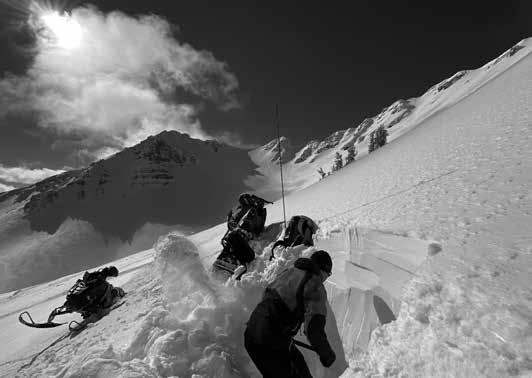

2.4.3 EQUIPMENT
The following equipment can be useful when observing snow profiles: 1. Probe
Snow shovel (flat bladed shovels are preferred)
Snow thermometer (calibrated regularly)
Ruler or probe graduated in centimeters
Magnifying instrument (10x or greater)
Checking Snow Depth
Check the snow depth with a probe before digging the obser vation pit and make sure the pit is not on top of a boulder, bush or in a depression. Careful probing can also be used to obtain a first indication of snow layering. Probing prior to digging is not necessary in a study plot, or when the snow is much deeper than your probe.
Digging the Snow Pit
Make the hole wide enough to facilitate all necessary observa tions and to allow shoveling at the bottom. Remember to exam ine the snow as you dig the pit as valuable information can be obtained during this process. In snow deeper than 2 m it may be advantageous to dig first to a depth of about 1.5 m, make the observations (such as stability tests) and then complete excava tion and observations to the necessary depth. The pit face on which the snow is to be observed should be in the shade. Cut the observation face in an adjacent sidewall vertical and smooth. On inclined terrain it is advantageous to make the observations on a shaded sidewall that is parallel to the fall line. Consider piling the debris on the downhill edge and sides to facilitate filling in the snow pit (Section 2.5.8).
Compass (adjusted for declination)
The thermometers should be calibrated to 0°C (32°F) periodi cally in a slush mixture after the free water has been drained. Glass thermometers must be checked for breaks in the mercury or alcohol columns before every use.
2.4.4 FIELD PROCEDURE
Equipment
Equipment used to measure or observe snow properties should be kept in the shade and/or cooled in the snow prior to use. Observers should wear gloves to reduce thermal contamination of measurements.
Recording
If there are two observers, the first observer can prepare the pit, while the second observer begins the observations (see Figures 2.7 and 2.9 for examples of field notes):
1. Record date, time, names of observers, location, eleva tion, aspect, slope angle, sky condition, precipitation, wind, surface penetrability (foot and ski penetration), and total snow depth.
2. Observe the air temperature to the nearest 0.5 degree in the shade about 1.5 m above the snow surface. Use a dry thermometer, wait several minutes, and then make sev eral readings about a minute apart to see if the thermom eter has stabilized. Record the temperature if there is no change between the two or more readings.
3. The convention for seasonal snow covers is to locate the zero point on the height scale at the ground. However, when the snow cover is deeper than about 3 m it is conve nient to locate the zero point at the snow surface. Setting
24 SNOWPACK OBSERVATIONS
6.
7.
8.
9.
10.
11.
12.
13.
14.
2.
3.
4.
5.
Crystal card
Field book
Snow saw
2 meter pre-knotted cord
Inclinometer
Density kit
Brush
Altimeter (calibrated regularly) 15. Topographic map 16. Global positioning system (GPS) unit 17. Camera
FIGURE 2.4 Targeted sites for snow profile observations. ! Doug Richmond and Mark Staples
the zero point at the snow surface, for test pits, eases comparisons with other snowpack observations made throughout the period. Observers should use whichever protocol fits their needs. In either case the total depth of the snowpack should be recorded when possible.
2.5 SNOWPACK OBSERVATIONS
2.5.1 SNOWPACK TEMPERATURE (T)
Observe snow temperature to the nearest fraction of a degree based on the accuracy and precision of the thermometers. Most field thermometers can measure snow temperature within 0.5 °C. Measure the snow surface temperature by placing the thermom eter on the snow surface; shade the thermometer. The tempera ture profile should be observed as soon as practical after the pit has been excavated.
Push the thermometer horizontally to its full length parallel to the surface into the snow (use the shaded side-wall of the pit on a slope). Wait at least one minute, re-insert close by, and then read the temperature while the thermometer is still in the snow. Shade the thermometer in order to reduce influence of radiation. One method is to push the handle of a shovel into the snow sur face so that the blade casts a shadow on the snow surface above the thermometer. Shading the snow above your thermometer is important when you are making temperature measurements in the upper 30 cm of the snowpack.
Measure the first sub-surface snow temperature 10 cm below the surface. The second temperature is observed at the next mul tiple of 10 cm from the previous measurement and from there in intervals of 10 cm to a depth of 1.4 m below the surface, and at 20-cm intervals below 1.4 m. Measure the snow temperatures at closer intervals when needed, as may be the case when the temperature gradients are strong, significant density variations exist, or when the temperatures are near to 0°C. When measur ing relatively small temperature variations, as is common around a crust or density discontinuity, greater accuracy and reliability in measurements may be possible by using a single thermome ter/temperature probe.
Begin the next observation while snow temperatures are being measured.
Compare thermometers first when two or more are used simul taneously. Place side by side in a homogeneous snow layer and compare the measurements. If they do not agree, only one of the thermometers should be used. Punch a hole in the snowpack with the metal case or a knife before inserting the thermometer into very hard snow and at ground surface. It is important to regularly check the accuracy of all thermometers by immersing them in a slush mixture after the free water has been drained; each should read 0°C. Prepare this mixture in a thermos and recalibrate or note variation from 0°C on the thermometer.
2.5.2 LAYER BOUNDARIES
Determine the location of each major layer boundary (Figure 2.5). Brushing the pit wall with a crystal card or a soft bristle paint brush will help to bring out the natural layering of the snowpack. Identify weak layers or interfaces of layers where a failure might occur. Record the distance from the layer boundary to the ground or snow surface depending on the convention being used.
Many operations find it useful to track specific features within the snowpack. Persistent weak layers or layers that are likely to produce significant avalanche activity (such as crusts, surface hoar, or near-surface facets) can be named with the date that they were buried. Some operations also find it useful to number each significant precipitation event and reference potential weak layers with these numbers or as interfaces between two num bered events.
Snow Hardness (R)
Observe the hardness of each layer with the hand hardness test. Record under “R” (resistance) the object that can be pushed into the snow with moderate effort parallel to the layer boundaries (Table 2.1).
Fierz and others (2009) suggest a maximum force of 10 to 15 newtons (1 to 1.5 kg force or about 2 or 3 pounds) to push the described object into the snow. Wear gloves when conducting hand hardness observations.
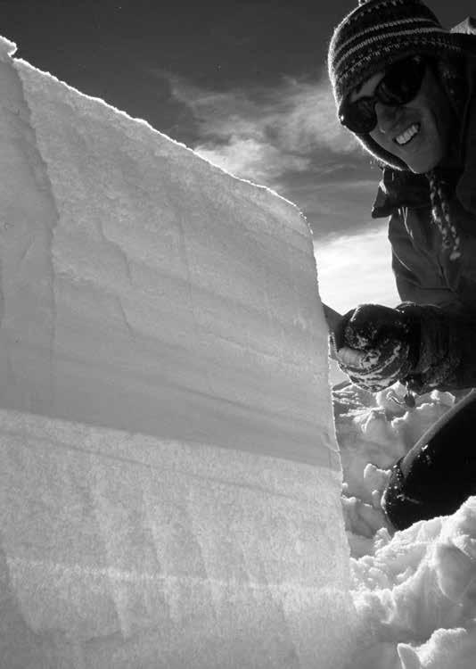
Slight variations in hand hardness can be recorded using + andqualifiers (i.e. P+, P, P-). A value of 4F+ is less hard than 1F-. Individual layers may contain a gradual change in hand hard ness value. These variations can be recorded in a graphical for mat (Figures 2.8 and 2.9), or by using an arrow to point from the upper value to the lower value (i.e. a layer that is soft on top and gets harder as you move down would read 4F+ → 1F).
FIGURE 2.5 The layered nature of a seasonal snow cover.
SNOWPACK OBSERVATIONS 25
! Bruce Tremper
SYMBOL HAND TEST TERM GRAPHIC SYMBOL
F Fist in glove Very low
4F Four fingers in glove Low
1F One finger in glove Medium
P Blunt end of pencil High
K Knife blade Very High
I Too hard to insert knife Ice �
N/O Not observed
2.5.3 GRAIN FORM (F)
The International Classification for Seasonal Snow on the Ground (Fierz and others, 2009) presents a classification scheme com posed of major and minor classes based on grain morphology and formation process. This scheme is used throughout this doc ument. Primary classes are listed in Tables 2.2 and 2.3. Subclasses are listed in Appendix F.
The major class of Precipitation Particles can be divided into minor classes that represent different forms of solid precipitation according to the International Classification for Seasonal Snow on the Ground. Commonly, the Precipitation Particles class (graphic symbol “+”) may be replaced by one of the classes in Table 2.2. Snow layers often contain crystals from more than one class or that are in transition between classes. In this case the observer can select primary and secondary classes for a single layer and place the secondary class in parentheses (e.g. a new snow layer composed of mostly plates with some needles could be listed as ()).
In warm weather the crystals may melt and their shape may change rapidly on the crystal card. In this case, a quick decision must be made and repeated samples taken from various depths of the same layer.
Snow layers often contain crystals in different stages of meta morphism (Figure 2.6). The classification should refer to the predominant type, but may be mixed when different types are present in relatively equal numbers. A maximum of two grain forms may be displayed for any single layer. The sub-classifica tion in Fierz, and others, 2009 has “mixed forms” classes that can be used by experienced observers who recognize grains that are in a transition stage between classes.
Illustrations of the various types of crystal shapes may be found in the following publications: LaChapelle, 1992; Perla, 1978; Colbeck and others, 1990; McClung and Schaerer, 2006, and Fierz and others, 2009.
Refer to the International Classification for Seasonal Snow on the Ground (Fierz and others, 2009) for complete descriptions of the grain forms listed here. (https://cryosphericsciences.org/ publications/snow-classification/)
2.5.4 GRAIN SIZE (E)
Determine the grain size in each layer with the aid of a crystal card. In doing so, disregard the small particles and determine
TABLE 2.2 Basic Classification of Snow on the Ground
SYMBOL DESCRIPTION
DATA CODE a
Precipitation Particles (New Snow) PP Machine Made Snow MM Decomposing and Frag mented Particles DF Rounded Grains (monocrystalline) RG Faceted Crystals FC Depth Hoar DH Surface Hoar SH Melt Forms MF Ice Formations IF
TABLE 2.3 Basic Classification of Snow in the Atmosphere
SYMBOL DESCRIPTION
DATA CODE Columns cl k Needles nd l Plates pl m Stellars and dendrites sd Irregular crystals ir o Graupel gp ▲ Hail hl q Ice pellets ip
Notes for Tables 2.2 and 2.3: Modifications to Fierz and others, 2009:
The use of a subscript “r” modifier is retained to denote rimed grains in the Precipitation Particles (PP) class and its subclasses except for gp, hl, ip, rm (Example: PP-r). The Decomposing and Fragmented Particles (DF) major class may be modified with "r". Subclasses for surface hoar are listed in Appendix F.
the average greatest extension of the grains that make up the bulk of the snow. Record the size or the range of sizes in milli meters in the column marked “E”. Record size to the nearest 0.5 mm, except for fine and very fine grains which may be recorded as 0.1, 0.3, or 0.5mm.
Where two distinct grain forms exist in a layer and their sizes are significantly different, list the size of the primary crystal form first followed by the size of the secondary class in parentheses. Example: 0.3 (2.5)
Where a range in sizes exists for any single grain form, specify the average and maximum size with a hyphen. Example: 0.5-1.5
26 SNOWPACK OBSERVATIONS
TABLE 2.1 Hand Hardness Index
Important distinctions between crystal sizes should be captured in field notes. However, excessive and unnecessary detail should be avoided.
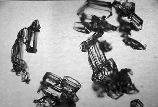
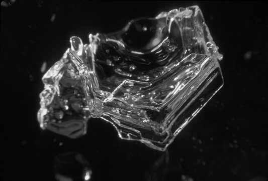

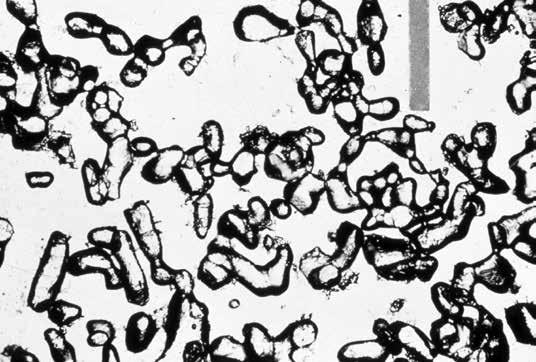
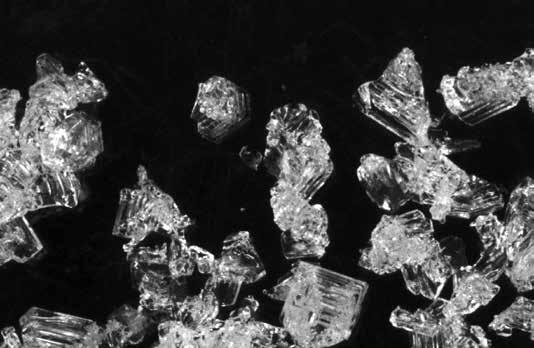
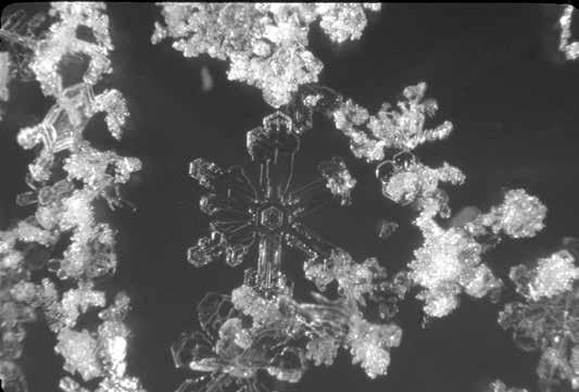
2.5.5 LIQUID WATER CONTENT (Θ)
Classify liquid water content of each snow layer that has a tem perature of 0°C. Gently squeeze a sample of snow with a gloved
hand and observe the reaction (Table 2.4); record in the column headed “θ” (theta).
2.5.6 DENSITY (
ρ)
Measure density of the snow in layers that are thick enough to allow insertion of the snow sampling device. Small samplers are more suitable for measuring the density of thin layers and larger samplers are better suited for depth hoar.
SNOWPACK OBSERVATIONS 27
FIGURE 2.6 Snow crystal formations found in seasonal snow cover. Clockwise from top left: Partially rimed new snow (a); Faceted grains formed near the snow surface (B); Rounded snow grains (d) ; Clustered melt forms (); Faceted snow grains (e); Depth hoar (D).
! Kelly Elder, Joe Stock, John Montagne, Ethan Greene, and Sam Colbeck
TABLE 2.4 Liquid Water Content of Snow (adapted from Fierz and others, 2009)
CLASS DEFINITION WATER CONTENT (BY VOLUME) SYMBOL DATA CODE
Dry
Usually the snow temperature (T) is below 0 °C but dry snow can occur at any temperature up to 0 °C. Disaggregated snow grains have little tendency to adhere to each other when pressed together. Difficult to make a snowball.
T = 0 °C. Water is not visible even at 10x magnifica tion. When lightly crushed, the snow has a distinct tendency to stick together. Snowballs are easily made. <3% I M Wet
Moist
T = 0 °C. Water can be recognized at 10x magnifica tion by its meniscus between adjacent snow grains, but water cannot be pressed out by moderately squeezing the snow in the hands (Pendular regime). 3-8% II W
T = 0 °C. Water can be pressed out by moderately squeezing the snow by hand, but there is some air confined within the pores (Funicular regime). 8-15% III V Slush
Very Wet
T = 0 °C. The snow is flooded with water and contains a relatively small amount of air. >15% IIII S
Insert the sample cutter into the pit wall, compacting the sam ple as little as possible. On angled slopes, sampling on the pit sidewall will make it easier to sample a single layer. Samples used for bulk density calculations can contain more than one snow layer; otherwise, be sure to sample one layer if possible. Trim the excess snow off the cutter and weigh. Either write down the mass under comments and calculate density later, or calculate density on site and note it in the column headed “ρ” (rho).
Calculate density as follows: Divide the mass (g) of the snow sample by the sample volume (cm3) and multiply by 1000 to express the result in kg/m3.
⍴( )kg mass of snow sample (g) m3 sample volume (cm3) = x 1000
The nomogram included on the final page (Section I.5) auto mates this calculation. Record as a whole number.
Practical methods for calculating snow density can be estab lished based on the snow volume sampled. For example, when using a 500 cm3 snow sampling tube multiply the mass of snow sample in the tube by 2, with a 250 cm3 sampler, multiply the snow sample mass by 4, etc.
2.5.7 STRENGTH AND STABILITY TESTS
Perform tests of strength and stability as appropriate (see Sections 2.6, 2.7, 2.9, and 2.10 for details on individual tests). It may be advantageous to perform multiple tests or iterations of a test.
2.5.8 MARKING THE SITE
If additional observations are to be made at this site, fill the pit
from a
profile.
28 SNOWPACK OBSERVATIONS
0% D
Fair Poor
Poor D epth Temp cm n °C °F AIR SFC
Depth Hard Grain Grain cm i n ness Type S ze Test Results an d Commen s Date: Tim e: Ref: Location: Elev: As pect: Slope Angle: Current P recip: Sky : Wind: C L M S X / B lowing Snow: Ext D r Loc PS/PF: / cm n Obs: Ty pe:
FIGURE 2.7 Example of field notes
test
Snow stability on s imilar slopes: Very Good Good
Very
GND
Snow Profile
Reference:
Date: Time: Observers:
Tes t Res ults and Comm ents I K P 1F 4F F G
Snow Layer Temperature (°C)
FIGURE 2.8 Hand-drawn full snow profile. Snow profile forms are provided in Appendix I.
SNOWPACK OBSERVATIONS 29
Location: Elev: Aspect: Slope Angle: Precip: Sky : Wind Dir: Speed: Blowing Snow: Ext Dir Loc PS: cm in PF: cm in Profile Type: D ept h Moist Form S iz e Dens ity H θ F E ρ (cm) (mm) (kg/m3)
and place a marker pole at the extreme edge. Pits dug in areas open to the public should be filled back in with snow.
2.5.9 GRAPHICAL SNOW PROFILE REPRESENTATION
Snow profiles can be represented graphically in a standard for mat for quick reference and permanent record (Figures 2.8 and 2.9).
1. Plot the snow temperatures as a curve; mark the air tem perature above the snow surface and use a dashed line to connect the two.
2. Plot the height of the snow layers to scale.
3. Use graphic symbols or data code for the shape of grains and liquid water content. Record N/O when the hardness or liquid water content was not observed or if it could not be determined (a blank implies fist hardness or dry snow respectively). Use of graphic symbols for hardness is optional.
4. Tabulate grain size and density with the values observed in the field.
5. Include written comments where appropriate. If possible, label important layers by their date of burial.
TABLE 2.5 Graphical Representation of Hand Hardness Index
HAND TEST
LENGTH OF BAR
Fist in glove Base Length Four fingers in glove 2X Base Length One finger in glove 4X Base Length Blunt end of pencil 8X Base Length Knife blade 16X Base Length Ice 20X Base Length
6. Include the results of appropriate strength and stability tests in the comments column.
7. Document grain form and size of the failure layer. Draw an arrow at the height of each observed failure and use a shorthand notation to describe the test. When multiple tests are performed the results of every test should be included.
FIGURE 2.9 Two different methods for recording field notes from a full profile.
30 SNOWPACK
OBSERVATIONS
Snow stability on s imilar slopes: Very Good Good Fair Poor Very Poor D epth Temp cm in C F AIR SFC GND Depth Hard Gra n Gra n cm n ness Type Size Test Resu ts an d Comments
Tim
Snow
on s imilar slopes: Very Good Good Fair Poor Very Poor D
h Temp cm n °C °F
GND
Date:
e: Ref: Location: Elev: As pect: Slope Angle: Current P recip: Sky : Wind: C L M S X B lowing Snow: Ext D r Loc PS/PF: / cm n Obs: Ty pe:
stability
ep
AIR SFC
Depth cm i n Date: T m e: Ref: Location: Elev: As pect: Slope Ang e: Current P recip: Sky : Wind: C L M S X / B owing Snow: Ext Dir Loc PS/PF: / cm i n Obs: Ty pe: F 4F 1F P K I
TABLE 2.6 A comparison of the categories in the Fracture Character and Shear Quality scales. (after van Herwijnen and Jamieson, 2003 and Birkeland, 2004)
FRACTURE CHARACTER CATEGORY SUBCLASS MAJOR CLASS TYPICAL SHEAR QUALITY
FRACTURE CHARACTER DATA CODE
Sudden Planar SP SDN Q1
Sudden Collapse SC SDN Q1
Progressive Compression PC RES Q2 or Q3
Resistant Planar RP RES Q2
Break BRK BRK Q3
Examples:
• ECTP24 SH(2–3) (Extended Column Test, propa gation on 24th tap, on 2–3 mm surface hoar)
• PST 57/100End FC(1.5)20221216 (Propagation Saw Test, cut was 57 cm long and then propagated to the end of 100 cm block, on a layer of 1.5 mm facets buried on December 16, 2022)
• RB6 (Q2) FC (1.5) (rutschblock score six, quality 2, on 1.5 mm faceted crystals)
• CT8 (Q1) DH (2.0) (Compression Test, on 8th tap, quality 1, on 2.0 mm depth hoar)
8. Plot the hand hardness test results as a horizontal bar graph (Figures 2.8 and 2.9). If a snowpack layer has vari able hand hardness, the length of the upper or lower ends of the bar can be shortened or lengthened and the connecting line angled or curved to reflect the variation (Figures 2.8 and 2.9). Changes in hardness category can be emphasized by using the bar lengths in Table 2.5. In regions where both weak layers and slabs are composed of very soft snow (1F or softer), it may be beneficial to plot the hard hardness index using the same distance to represent each category.
2.6 CHARACTERIZING FRACTURES IN COLUMN AND BLOCK TESTS
Many of the stability tests described in the following sections yield some indication of the load required to produce a frac ture. Fracture is the process of crack propagation. In addition to the magnitude of the load, observing the nature of the frac ture can improve estimations of snow stability and can, in par ticular, reduce false-stable results (Johnson and Birkeland, 1998; Birkeland and Johnson, 1999; Johnson and Birkeland, 2002; Birkeland and Johnson, 2003; van Herwijnen and Jamieson, 2002; van Herwijnen, 2003). Both methods described below may be included with the results of a column or block test (see Section 2.7) and provide additional information about the sta bility of the snow slope. All the research with these methods has been conducted using compression-type tests such as the com pression, stuffblock, and Rutschblock Tests.
The methods described in this section provide a qualita tive assessment of the fracture (crack propagation) potential. Although the definitions and approach differ, the phenomena they describe are essentially identical (Table 2.6). Both methods
require experienced observers to make somewhat subjective assessments, especially when trying to determine whether a pla nar fracture is sudden (SP/Q1) or resistant (RP/Q2). Members of an operational program should select the method that works best for their application and periodically compare their ratings to ensure consistency.
2.6.1
SHEAR QUALITY
Shear Quality was developed by avalanche workers at the Gallatin National Forest Avalanche Center (Southwest Montana) to assess fracture (crack propagation) potential. It can be used with many of the stability tests in this chapter, but is not recommended for use with the Extended Column Test and Propagation Saw Test, which were developed specifically to assess crack propagation potential.
Procedure
1. Conduct any of the stability tests described in this chapter.
2. Carefully observe how the fracture occurs and examine the nature of the fracture plane.
3. Record the results in accordance with the shear quality definitions (Table 2.7).
Recording
The results can be included at the end of a shear test result. Example: A rutschblock score of 2 with a shear quality of 1 would be recorded as RB2(Q1). A Compression Test that fractured with 5 taps from the elbow producing a rough shear plane would be recorded as CT15(Q3).
2.6.2 FRACTURE CHARACTER
Fracture Character was developed by the Applied Snow and Avalanche Research Group at the University of Calgary to assess fracture (crack propagation) potential. It can be used with many of the stability tests in this chapter and other tests that load a small column of snow until a fracture appears, but is not recom mended for use with the Extended Column Test and Propagation Saw Test.
Fracture character is best observed in tests performed on a small isolated column of snow where the objective is to load the column until it fractures, or fails to fracture. The front face and side walls of the test column should be as smooth as possible. The observer should be positioned in such a way that one side wall and the entire front face of the test column can be observed.
SNOWPACK OBSERVATIONS 31
TABLE 2.7 Shear Quality Ratings
DESCRIPTION DATA CODE
Unusually clean, planar, smooth and fast shear surface; weak layer may collapse during fracture. The slab typically slides easily into the snow pit after weak layer fracture on slopes steeper than 35 degrees and sometimes on slopes as gentle as 25 degrees. Tests with thick, collapsible weak layers may exhibit a rougher shear surface due to erosion of basal layers as the upper block slides off, but the initial fracture was still fast and mostly planar.
“Average” shear; shear surface appears mostly smooth, but slab does not slide as readily as Q1. Shear surface may have some small irregularities, but not as irregular as Q3. Shear fracture occurs throughout the whole slab/weak layer interface being tested. The entire slab typically does not slide into the snow pit.
Shear surface is non-planar, uneven, irregular and rough. Shear fracture typically does not occur through the whole slab/weak layer interface being tested. After the weak layer fractures the slab moves little, or may not move at all, even on slopes steeper than 35 degrees.
TABLE 2.8 Fracture Character Ratings
Q2
FRACTURE CHARACTER CATEGORY SUBCLASS DATA CODE MAJOR CLASS DATA CODE
A thin planar* crack suddenly crosses column in one loading step AND the block slides easily** on the weak layer Sudden planar SP Sudden SDN
Crack crosses the column with a single loading step and is associated with a noticeable collapse of the weak layer. Sudden collapse SC Sudden SDN
A crack of noticeable thickness (non-planar fractures often greater than 1cm), which usually crosses the column with a single loading step, fol lowed by step-by-step compression of the layer with subsequent loading steps.
Planar or mostly planar shear surface that requires more than one loading step to cross column and/ or the block does NOT slide easily** on the weak layer.
Progressive compression PC Resistant RES
Resistant planar RP Resistant RES
Non-planar; irregular fracture. Non-planar break BRK Break BRK
Note:* “Planar” based on straight fracture lines on front and side walls of column. ** Block slides off column on steep slopes. On low-angle slopes, hold sides of the block and note resistance to sliding.
Attention should be focused on weak layers or interfaces identi fied in a profile or previous snowpack.
Procedure
1. Conduct a stability test.
2. Carefully observe how the fracture occurs in the target weak layer. For tests on low-angled terrain that produced planar fractures, it may be useful to slide the two shear surfaces across one another by carefully grasping the two sides of the block and pulling while noting the resistance.
3. Record the results in accordance with the definitions in Table 2.8.
Recording
The results can be included at the end of a stability test result.
Example:
A sudden fracture in a Rutschblock Test with a score of 2 would be recorded as RB2(SDN). A Compression Test that fractured with 5 taps from the elbow producing a resistant planar fracture would be recorded as CT15(RP).
32 SNOWPACK OBSERVATIONS
Q1
Q3
2.7 COLUMN AND BLOCK TESTS
2.7.1 SITE SELECTION
Test sites should be safe, geographically representative of the ava lanche terrain under consideration, and undisturbed. For exam ple, to gain information about a wind-loaded slope, find a safe part of a similarly loaded slope for the test. The site should not contain buried ski tracks or avalanche deposits. In general, the site should be farther than about one tree length from trees where buried layers might be disturbed by wind action or by clumps of snow that have fallen from nearby trees (imagine a line drawn between a treetop and the snow surface, the acute angle between that line and the horizontal should be at most 45°). Föhn (1987a) recommends slope angles of at least 30º for Rutschblock Tests, but stability tests done on 25º–30º slopes can yield useful infor mation. Be aware that near the top of a slope snowpack layering and hence test scores may differ from the slope below.
In the past few decades, interest in understanding and doc umenting spatial variations in the physical properties of snow has increased in both the research and applied communities (Schweizer et al., 2008). The general guidelines outlined in the paragraph above remain part of good field practice. However, there is increasing evidence that making more observations is an effective strategy for avalanche operations and can help min imize the frequency of false-stable situations (Birkeland and Chabot, 2006). Both scientists and field workers should main tain a high level of curiosity and continue to search for signs and areas of instability, even during periods when the snow appears to be stable.
2.7.2 SHOVEL SHEAR TEST
Objective
Identification of the location of weak layers is the primary objec tive of the Shovel Shear Test. The test provides:
1. Information about the location where the snow could fail in a shear.
2. A qualitative assessment of weak layer strength. It is best applied to identify buried weak layers, and it does not usually produce useful results in layers close to the snow surface.
Procedure
A shovel is the only equipment required for the Shovel Shear Test. However, a snow saw will make cutting the snow column easier and more precise.
1. Select a safe site that has undisturbed snow and is geo graphically representative of slopes of interest.
2. Expose a fresh pit wall by cutting back about 0.2 m from the wall of a full snow profile or test profile.
3. Observers can remove very soft snow (fist hardness) from the surface of the area where the test is to be carried out if necessary.
4. On the snow surface mark a cross section of the column to be cut, measuring 30 cm wide and 30 cm in the upslope direction (approximately the width of the shovel blade to be used).
5. Cut a chimney wide enough to allow the insertion of the saw on one side of the column and a narrow cut on the other side.
6. Make a vertical cut at the back of the column and leave the
cutting tool (saw) at the bottom for depth identification. The back-cut should be 0.7 m deep maximum and end in medium hard to hard snow if possible.
7. Carefully insert the shovel into the back-cut no farther than the heel of the shovel. Hold the shovel handle with both hands and apply an even force in the down-slope (slope parallel) direction (Figure 2.10). Be careful not to pry the column away from the snow pit wall.
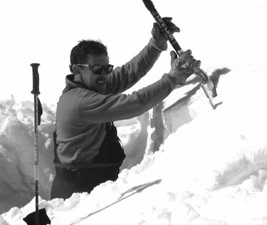
8. When the column breaks in a smooth shear plane above the low end of the back-cut, mark the level of the shear plane on the rear (standing) wall of the back-cut.
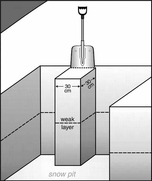
SNOWPACK OBSERVATIONS 33
FIGURE 2.10 Photograph and schematic of the Shovel Shear Test. ! Kelly Elder
Loading Steps and Shovel Shear Test Scores
TERM DESCRIPTION
EQUIVALENT SHEAR STRENGTH (PA) DATA CODE
Collapse Block collapses when cut STC
Very Easy Fails during cutting or insertion <100 STV
Easy Fails with minimum pressure 100-1000 STE
Moderate Fails with moderate pressure 1000-2500 STM
Hard Fails with firm sustained pressure 2500-4000 STH
No Shear No shear failure observed STN
9. After a failure in a smooth shear layer or an irregular sur face at the low end of the back-cut, or when no failure occurs, remove the column above the bottom of the backcut and repeat steps 6 to 8 on the remaining column below.
10. Repeat the test on a second column with the edge of the shovel 0.1 m to 0.2 m above the suspected weak layer.
11. Measure and record the depth of the shear planes if they were equal in both tests. Repeat steps 4 to 9 if the shear planes were not at the same depth in both tests.
12. If no break occurs, tilt the column and tap (see Section 2.9.4).
13. Use Table 2.9 to classify the results of the test.
14. Observe and classify the crystal form and size at the shear planes. (Often a sample of the crystals is best obtained from the underside of the sheared block.)
15. Record the results of the test with the appropriate data code from Table 2.9 along with the height, and grain type and size of the weak layer (i.e. “STE@125cm↑e1mm” would be an easy shear on a layer of 1 mm faceted grains 125 cm above the ground).
Results
The ratings of effort are subjective and depend on the strength and stiffness of the slab, dimensions of the shovel blade and han dle, and the force applied by the tester. Observers are cautioned that identification of the location of weak layers is the primary objective of the Shovel Shear Test.
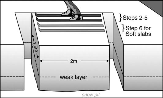
2.7.3 RUTSCHBLOCK TEST
The rutschblock (or glide-block) test was developed in Switzerland in the 1960s. This section is based on analysis of Rutschblock Tests in Switzerland (Föhn, 1987a; Schweizer, 2002) and Canada (Jamieson and Johnston, 1993a and 1993b).
Objective
The Rutschblock is a good slope test for layers up to 1 m deeper than ski penetration. The test does not eliminate the need for snow profiles or careful field observations, nor does it, in general, replace other slope tests such as slope cutting and explosive tests.
Procedure
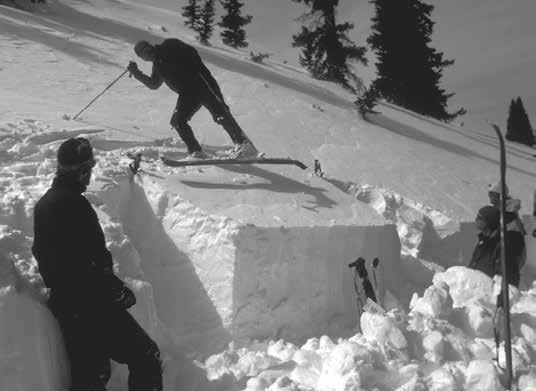
A shovel is required. Ski pole mounted saws or rutschblock cut ting cords (8 meters of 3–4 mm cord with knots every 20–30 cm) save time isolating the block in soft or medium-hard snowpacks. However, extra care is required to ensure the block has straight
edges. Large rutschblock saws are useful to cut knife-hard crusts. The Rutschblock Test can be performed with either skis or a snowboard.
1. Select a safe site that has undisturbed snow and is geo graphically representative of the slopes of interest.
2. Observe a snow profile and identify weak layers and potential slabs.
3. Excavate a pit wall, perpendicular to the fall line, that is wider than the length of the tester’s skis (2 m minimum)
34 SNOWPACK OBSERVATIONS
FIGURE 2.12 Schematic of the Rutschblock Test (after Jamieson and Johnston, 1993a).
FIGURE 2.11 Stepping onto the block during a Rutschblock Test. ! Kelly Elder
TABLE 2.9
Rutschblock Loading Steps and Scores
FIELD SCORE LOADING STEP THAT PRODUCES A CLEAN FRACTURE SURFACE DATA CODE
1 The block slides during digging or cutting. RB1
2 The skier approaches the block from above and gently steps down onto the upper part of the block within 35 cm of the upper wall (Figure 2.11). RB2
3 Without lifting the heels, the skier drops once from straight leg to bent knee position (feet together), pushing downwards and compacting surface layers. RB3
4 The skier jumps up and lands in the same compacted spot. RB4
5 The skier jumps again onto the same compacted spot. RB5
6
For hard or deep slabs, remove skis and jump on the same spot. For soft slabs or thin slabs where jumping without skis might penetrate through the slab, keep skis on, step down another 35 cm (almost to mid-block) and push once then jump three times. RB6
7 None of the loading steps produced a smooth slope-parallel failure. RB7
4. Mark the width of the block (2 m) and the length of the side cuts (1.5 m) on the surface of the snow with a ski, ruler, etc. The block should be 2 m wide throughout if the sides of the block are to be dug with a shovel. However, if the side walls are to be cut with a ski, pole, or saw, the lower wall should be about 2.1 m across and the top of the side cuts should be about 1.9 m apart.
5. This flaring of the block ensures it is free to slide without binding at the sides.
6. Dig out the sides of the block, or make vertical cuts down the sides using the lines marked on the snow surface.
7. Cut the downhill face of the block smooth with a shovel.
8. Using a ski or snow saw make a vertical cut along the uphill side of the block so that the block is now isolated on four sides.
9. Rate any fractures that occur while isolating the block as RB1.
10. Conduct loading steps as described in Table 2.10, and record the results with the appropriate rutschblock score as well as the release type that occurred during the test (Table 2.11). A field book notation for recording rutschblock results is shown in Figure 2.13.
11. Rate any identified weak layers that did not fracture as no failure (RB7).
12. Record rutschblock results in a field book along with per tinent site information using the method shown in Figure 2.13 or the data codes in Tables 2.10 and 2.11.
Results
The rutschblock only tests layers deeper than ski penetration. For example, a weak layer 20 cm below the surface is not tested by skis that penetrate 20 cm or more. Higher and more variable rutschblock scores are sometimes observed near the top of a slope where the layering may differ from the middle and lower part of the slope (Jamieson & Johnston, 1993). Higher scores may contrib ute to an incorrect decision. The rutschblock may not effectively test weak layers deeper than about 1 m below ski penetration.
TABLE 2.11 Release Type Ratings for the Rutschblock Test
TERM DESCRIPTION DATA CODE
Whole block 90 — 100% of the block WB
Most of block 50 — 80% of the block MB
Edge of block 10 — 40% of the block EB
FIGURE 2.13 A field notebook method for recording a rutschblock score, release type, shear quality (center of box) along with the slope angle, elevation, crystal form and size, depth of weak layer, and as pect (clockwise from top). Arrows can be used to indicate whether the depth of the weak layer was measured from the snow surface or the ground (i.e. 68 cm below the snow surface).
Schweizer, McCammon and Jamieson (2008) found that rutschblock scores combined with release type correlated well with observed avalanche occurrence. Johnson and Birkeland (2002) found that combining rutschblock scores with shear qual ity ratings reduced the number of false-stable results.
Research demonstrates that rutschblock results can vary over short distances. As such, interpret the results of any stability test in conjunction with snowpack and weather histories, and other snowpack and avalanche information.
SNOWPACK OBSERVATIONS 35
TABLE 2.10
2.7.4 COMPRESSION TEST
The Compression Test was first used by Parks Canada wardens working in the Canadian Rockies in the 1970s. The following procedure was developed by the University of Calgary avalanche research project in the late 1990s. Similar tests have been devel oped elsewhere.
Objective
The Compression Test attempts to locate weak layers in the upper snowpack (~ 1m) and provide an indication of the trig gering likelihood on nearby slopes with similar snowpack con ditions. The tester places a shovel blade on top of an isolated snow column and taps the blade, causing weak layers within the column to fracture. These fractures can be seen on the smooth walls of the column. Compression tests are typically performed on sloping terrain. Tests of distinct, collapsible weak layers can be performed on level study plots.

Procedure
A shovel is the only piece of equipment required for the Compression Test. However, a snow saw will make cutting the column of snow easier and more precise.
1. Select a safe site that has undisturbed snow and is geo graphically representative of the slopes of interest.
2. Isolate a column of snow 30 cm wide with a 30 cm ups lope dimension that is deep enough to expose potential weak layers on the smooth walls of the column. Field tests have indicated that the size of the shovel blade used
has minimal impact on test outcome (Jamieson, 1996). A depth of 100–120 cm is usually sufficient since the Compression Test rarely produces fractures in deeper weak layers. Taller columns tend to wobble during tap ping, potentially producing misleading results for deep weak layers (Jamieson, 1996).
3. Rate any fractures that occur while isolating the column as Very Easy (CTV).
4. If the snow surface slopes, you can remove a wedge of snow to level the top of the column.
5. Place a shovel blade on top of the column. Tap 10 times with fingertips, moving hand from wrist and note the number of taps required to fracture the column (1 to 10).
6. If during tapping the column fails, leave the failed portion on top of the column, provided it does not compromise other observations. If the upper part of the column slides off or no longer “evenly” supports further tapping on the column, remove the damaged part of the column and continue tapping.

7. Tap 10 times with the fingertips or knuckles moving fore arm from the elbow, and note the total number of taps required to fracture the column (11 to 20). While moder ate taps should be harder than easy taps, they should not be as hard as one can reasonably tap with the knuckles.
8. Finally, hit the shovel blade moving the arm from the shoulder 10 times with open hand or fist and note the total number of taps required to fracture the column (21 to 30). If the moderate taps were too hard, the operator
36 SNOWPACK OBSERVATIONS
FIGURE 2.14 Schematic and photograph of the Compression Test. ! Bruce Tremper
Loading Steps and Compression Test Scores
TERM DESCRIPTION
Very Easy Fractures during cutting CTV
Easy Fractures within 10 light taps using finger tips only
Moderate Fractures within 10 moderate taps from the elbow using finger tips
CT1 to CT10
CT11 to CT20
Hard Fractures within 10 firm taps from whole arm using palm or fist CT21 to CT30
No Fracture Does not fracture CTN
will often try to hit the shovel with even more force for the hard taps and may hurt their hand.
9. Rate any identified weak layers that did not fracture as No Fracture (CTN).
10. Record the depth of the snowpack that was tested. For example, if the top 110 cm of a 200 cm snowpack was tested (30 taps on a column, 110 cm tall) and the only result was a failure on the 15th tap, 25 cm below the sur face, then record “CT15 @25 cm; Test depth 110 cm, or TD 110”. This clearly indicates that no fracture occurred from 25–110 cm below the surface and that the snow pack between 110 cm and 200 cm was not tested with the Compression Test. Operations that always test the same depth of the snowpack, (e.g. top 120 cm) may omit the test depth.
Results
Limitations of the Compression Test include sampling a relatively small area of the snowpack and the variability in force applied by different observers. A greater understanding of these limitations can be gained by conducting more than one Compression Test in a snow profile and performing side by side tests with other observers.
Deeper weak layers are generally less sensitive to taps on the shovel, resulting in higher ratings. Similarly, deeper weak layers are less sensitive to human triggering.
Experience and research in the Rocky and Columbia Mountains of Western Canada indicates that human-triggered avalanches are more often associated with "Easy" (1–9 taps) frac tures than with "Hard" (20–30 taps) fractures or with layers that do not fracture (Jamieson, 1996). Sudden fractures (SC, SP, Q1) that show up on the column walls as straight lines identify the failure layers of nearby slab avalanches more often than nonplanar or indistinct failure surfaces (BRK, Q3) (vanHerwijnen & Jamieson, 2003).
TABLE 2.13 Loading Steps and Deep Tap Test Scores
Research demonstrates that Compression Test results can vary over short distances. As such, interpret the results of any stabil ity test in conjunction with snowpack and weather histories, and other snowpack and avalanche information.
2.7.5 DEEP TAP TEST
The Deep Tap Test was developed by the Applied Snow and Avalanche Research group at the University of Calgary. The test was developed to address very deep weak layers that are difficult to assess with other column and block tests.
Objective
The primary objective of the Deep Tap Test is to determine the type of fracture that occurs in a weak layer that is too deep to fracture consistently in the Compression Test. In addition, one may observe the tapping force required for fracture to occur.
Procedure
A shovel is the only piece of equipment required for the Deep Tap Test. However, a snow saw will make cutting the column of snow easier and more precise.
1. Using a profile or other means, identify a weak snowpack layer, which is overlaid by 1F or harder snow and which is too deep to fracture consistently in the Compression Test.
2. Prepare a 30 cm x 30 cm column as for a Compression Test (note that the same column can be used after a Compression Test of the upper layers, provided the Compression Test did not disturb the target weak layer). To reduce the likelihood of fractures in weak layer below the target layer, such as depth hoar at the base of the snowpack, it may be advanta geous not to cut the back wall more than a few centimeters below the target weak layer.
3. Remove all but 15 cm of snow above the weak layer, mea sured at the back of the sidewall. This distance should be constant, regardless of the slope angle.
TERM DESCRIPTION DATA CODE
Very Easy Fractures during cutting DTV
Easy Fractures within 10 light taps using finger tips only
DT1 to DT10
Moderate Fractures within 10 moderate taps from the elbow using finger tips DT11 to DT20
Hard Fractures within 10 firm taps from whole arm using palm or fist DT21 to DT30
No Fracture Does not fracture DTN
SNOWPACK OBSERVATIONS 37
TABLE 2.12
DATA
CODE
4. Place the shovel blade (facing up or facing down) on top of the column. Tap 10 times with fingertips, moving hand from wrist and note the number of taps required to frac ture the column (1 to 10).
5. Tap 10 times with the fingertips or knuckles moving your forearm from the elbow, and note the total number of taps required to fracture the column (11 to 20). While moderate taps should be harder than easy taps, they should not be as hard as one can reasonably tap with the knuckles.
6. Finally, hit the shovel blade moving arm from the shoul der 10 times with open hand or fist and note the total number of taps required to fracture the column (21 to 30). If the moderate taps were too hard, the operator will often try to hit the shovel with even more force for the hard taps–and may hurt his or her hand.
7. Record the results as described in Table 2.13. Observers may also include the total depth of the weak layer below the snow surface at the location of the test.
8. Use one of the methods in Section 2.6 to describe the type of fracture observed during the test. This information is important for deep persistent weak layers.
Results
While very effective for testing deeper weak layers, the number of taps required to initiate a fracture in the Deep Tap Test has not been correlated with human-triggered avalanches or avalanches on adjacent slopes.
2.7.6 EXTENDED COLUMN TEST
The Extended Column Test (ECT) was developed in Colorado and New Zealand in 2005 and 2006. The ECT was tested in the continental and intermountain snow climates of the U.S. (Simenhois and Birkeland, 2007; Hendrikx and Birkeland, 2008; Birkeland and Simenhois, 2008), the Swiss Alps (Winkler and Schweizer, 2009), the Spanish Pyrenees (Moner et al., 2008) and New Zealand’s Southern Alps (Simenhois and Birkeland, 2006, Hendrikx and Birkeland, 2008).
Objective
The ECT tests the propensity for weak layer crack initiation and propagation in the upper portion of the snowpack. The tester tries to initiate a weak layer crack by applying dynamic load to a shovel blade placed at the end of an isolated column. (Figure 2.16) Once initiated, the key observation in the test is whether the crack immediately propagates across the entire column. The
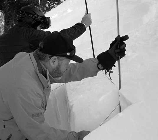
TABLE 2.14 Loading Steps and Extended Column Test Scores
DESCRIPTION
ECT identifies crack initiation during the loading steps and then whether that crack propagates across the column.
Procedure
A shovel is required, and a snow saw will make cutting the col umn easier and more precise. Also required are 1–2 snow probes or ski poles and 2 m of 2–4 mm cord knotted every 20–30 cm, or a snow saw with extension.
1. Select a safe site that has undisturbed snow and is geo graphically representative of the slope of interest.
2. Isolate a column of snow 90 cm wide in the cross slope dimension and 30 cm deep in the upslope dimension that is deep enough to expose potential weak layers. Depth should not exceed 120 cm since the loading steps rarely affect deeper layers.
3. Rate any fractures that cross the entire column while isolating it as ECTPV.
4. If the snow surface slopes and the surface snow is hard, remove a wedge of snow to level the top of the column at one edge.
5. Place the shovel blade on one side of the column. Tap 10 times moving hand from the wrist and note the number of taps it takes to initiate a fracture and whether the crack immediately propagates across the entire column (1 to 10).
DATA CODE
ECTPV Fracture initiates and propagates across the entire column on the ## tap
Fracture propagates across the entire column during isolation
ECTP## Fracture initiates on the ## tap, but does not propagate across the entire column. It either frac tures across only part of the column (observed commonly), or it initiates but takes additional loading to propagate across the entire column (observed relatively rarely).
No fracture occurs during the test
ECTN##
ECTX
38 SNOWPACK OBSERVATIONS
FIGURE 2.15a Cutting an ECT. ! Don Sharaf
6. Tap 10 times with the fingertips or knuckles moving fore arm from the elbow and note the number of taps it takes to initiate a fracture and whether the crack immediately propagates across the entire column (11 to 20).
7. Finally, hit the shovel blade moving arm from the shoulder 10 times with open hand or fist. Note the number of taps it takes to initiate a fracture and whether the crack immedi ately propagates across the entire column (21 to 30).
8. If a fracture occurs and you wish to keep testing, remove the failed portion of the block and continue with the next loading step.
9. If no fractures occurred within all loading steps, rate the test as ECTX.
10. If a crack initiated on a weak layer on the ## tap but did not propagate across the entire column rate that layer as ECTN##.
11. If a crack initiated and propagated across the entire col umn on the ## tap rate that layer as ECTP##.
Results
The ECT has become a popular test for professionals and recre ationists. Note that the ECT is not a good tool for assessing frac ture propagation potential on weak layers deeper than 100–150 cm
TABLE 2.15 Propagation Saw Test Description and Data Codes
OBSERVED RESULT
Propagation to end
Slab fracture
Self-arrest
No fracture occurs
DESCRIPTION
(Hoyer et al., 2016). In cases where a fracture is not initiated, tests in different locations or other stability tests are recommended.
As with other tests, research demonstrates that ECT results can vary over short distances. As such, interpret the results of any stability test in conjunction with snowpack and weather his tories, and other snowpack and avalanche information.

2.7.7 PROPAGATION SAW TEST
The Propagation Saw Test (PST) was simultaneously developed in Canada (Gauthier and Jamieson, 2007) and in Switzerland (Sigrist, 2006). The PST has been tested in Canada’s Columbia Mountains, in the Swiss Alps, and in Colorado’s continental snowpack (Birkeland and Simenhois, 2008).
Objective
The PST tests weak layer crack propagation propensity, and has been used on weak layers buried up to 250 cm deep. The tester isolates a column and initiates a fracture by dragging a snow saw along the weak layer in the uphill direction.
Procedure
A shovel and a snow saw with a blade at least 30 cm long and 2 mm thick are required for the PST. For layers deeper than 30
DATA CODE
The crack propagates in the weak layer in front of the saw uninterrupted to end of the column End
The crack propagates in the weak layer in front of the saw and stops where it meets a crack through the overlying slab
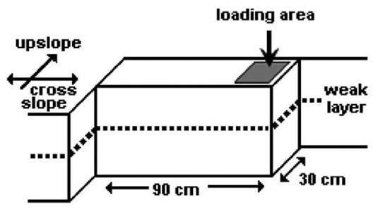
The crack propagates in front of the saw but self-arrests somewhere along the weak layer before reaching the end of the column
Saw runs through the weak layer for the en tire length of the column without producing a crack that extends on its own
SF
Arr
SNOWPACK OBSERVATIONS 39
FIGURE 2.15b and c Schematic and photograph of the Extended Column Test. ! Ron Simenhois and Karl Birkeland
X
FIGURE 2.16 Schematic showing the PST column (a) and the observable results of propagation to end (b), slab fracture (c), and self arrest (d) (after Gauthier and Jamieson, 2007).
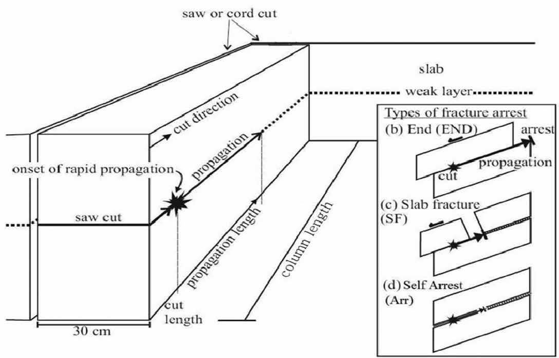
FIGURE 2.17 The PST process (left to right): isolating the column with probes and cord; identifying the weak layer and preparing to cut; drag ging the saw along the weak layer until the onset of propagation. Lightly brushing the weak layer with a glove or brush before cutting helps the operator follow the layer along the column. ! Applied Snow and Avalanche Research, University of Calgary
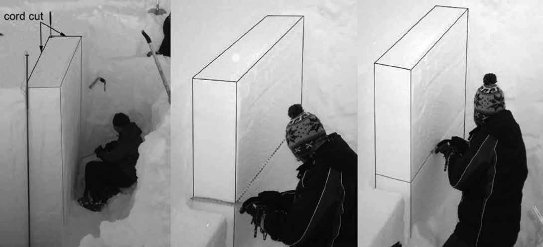
40 SNOWPACK OBSERVATIONS
cm, 1–2 snow probes and 3–5 m of 3–4 mm cord knotted every 20–30 cm are recommended.
The PST procedure involves three main steps (after Gauthier and Jamieson, 2007): identifying the weak layer of interest, isolating and preparing the test column, and performing and recording the results.
1. Select a safe site that has undisturbed snow and is geo graphically representative of the slope of interest.
2. For weak layer depths less than 100 cm, isolate a column 30 cm wide across the slope and 100 cm upslope to a depth of at least the depth of the weak layer. The cuts at the upslope and downslope end of the column should be cut vertically. For layers deeper than the saw is long, two adjacent walls can be cut with a cord between probes. When the weak layer is >100 cm deep the column length is equal to the weak layer depth in the upslope direction.
3. To identify the weak layer clearly, mark it with a glove, a brush or a crystal card along the exposed column wall.
4. Drag the blunt edge of the saw upslope through the weak layer at 10–20 cm/s until the crack propagates ahead of the saw, at which point the tester stops dragging the saw and marks the spot along the layer where propagation began.
5. After observations are complete, remove the column and check that the saw scored the weak layer in the wall behind the test column. If the saw deviated from the weak layer, the test should be repeated.
Results
When a fracture propagates ahead of the saw, one of the three results described in Table 2.15 can be observed. PSTs are then recorded as follows: 'PST x/y (Arr, SF, or End)' where x is the length of the saw cut when propagation starts and y is the length of the isolated column. Units are recorded in centimeters. It is recommended to record slope angle at the test site if it is not done on a 30–40 degree slope. Propagation to End occurs on flat as well as inclined slopes.
Crack propagation is considered to be likely if the fracture propagates to the end of the column along the same layer and initiates when the length of the saw cut is less than 50% of the length of the column (Gauthier & Jamieson, 2008). Otherwise crack propagation is considered unlikely. An example of a result that indicates high propagation propensity 'PST 34/100 (End)'.
The PST is one of the few tools — besides explosive testing — that can be used to assess the crack propagation propensity of deeply buried weak layers. The PST may not work as well for weak layers that are difficult to cut with the saw’s blunt edge (Birkeland & Simenhois, 2008; Gauthier & Jamieson, 2008).
TABLE
2.16 Slope Cut Test Description and Data Codes
As with other stability tests, PST results can vary over short distances. As such, interpret the results of any stability test in conjunction with snowpack and weather histories, and other snowpack and avalanche information.
2.8 SLOPE CUT TESTING
Slope cutting can provide valuable snowpack information. Safety is the primary concern when attempting slope cuts; inexperi enced observers should not perform this type of testing. There are many approaches and tricks of the trade that can be applied to slope cutting. All of them are beyond the scope of this manual. Slope cutting techniques should only be taught in the field or as on the job training. More information on slope cuts can be found in Tremper (2008), McClung and Schaerer (2006) and Perla and Martinelli (1976).
TERM DESCRIPTION DATA CODE
No release No result SCN
Whumpfing
Slope cut produces a collapse in the snowpack SCW
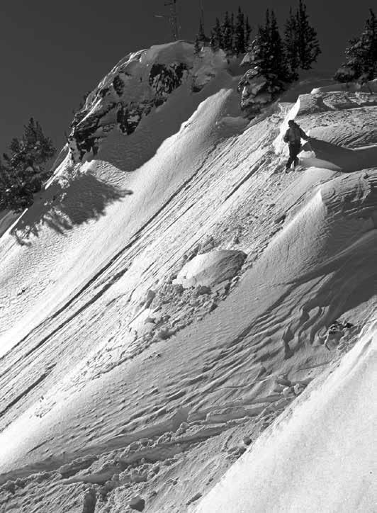
Cracking Slope cut produces shooting cracks SCC
Avalanche Slab Slope cut produces a slab avalanche SCS
Avalanche Loose Slope cut produces a loose snow or sluff avalanche SCL
SNOWPACK OBSERVATIONS 41
FIGURE 2.18 Slope cut producing a small slab avalanche. ! Bruce Tremper
Objective
Slope cutting can provide valuable information on snowpack sta bility. A tester attempts to initiate failure on a given slope by quickly applying a dynamic force (with skis, snowboard, snowmobile, etc.) to a test slope and then escaping to a safe location (Figure 2.18).
Procedure
1. Choose a relatively small slope that is representative of the starting zones you wish to learn about.
2. Place one or more people in zones of safety that allow them to observe the entire cut and avalanche path, if possible.
3. Begin from a zone of safety.
4. Examine the starting zone and choose a line that crosses rel atively high on the slope and ends in a zone of safety.
5. Travel along the line maintaining enough speed to cross the slope in one fast motion. The tester can bounce or jump during the cut to increase the load on the slope.
6. Exit the slope to a zone of safety.
Results
Record the results of the test using the data codes listed in Table 2.16 along with the aspect and angle of the slope. When a slope cut produces a slab avalanche the avalanche size (Relative and/ or Destructive) can be included in the data code. Additional information about the terrain and resulting avalanche can be recorded in comments as needed.
Example:
SCW35NE — Test produced a collapse (whumpf) on a 35° northeast-facing slope.
SCL40S — Test produced a sluff on a 40° south-facing slope. SCN30N — Test produced no result on a 30° north-fac ing slope.
SCS45NWR3D2 — Test produced a slab avalanche on a 45° northwest-facing slope. The avalanche was medium size for the path but large enough to injure or kill a person.
2.9 NON-STANDARDIZED SNOW TESTS
All of the stability tests described in Chapter 2 were developed from many years of work by many observers. Each test went through several iterations before a standard procedure was established. Field practitioners and researchers eventually wrote protocols and conducted research on these tests to provide infor mation on their response and suitability.
In addition to the standardized tests, there are many other tests that do not have specific field protocols. In this section, some of the more common non-standardized snow tests and suggested methods for communicating their results are presented. Field workers who are not satisfied with the standardized tests are encouraged to use additional methods for determining physi cal properties of the snowpack. As new methods evolve and we learn more about their responses and limitations, those methods may become standard practice.
2.9.1 COMMUNICATING THE RESULTS OF NON-STANDARDIZED SNOW TESTS
There is no standard method for communicating the results of non-standardized tests. A common method is to rate the amount of force required to produce a fracture using the descriptors Easy,
Moderate, or Hard (with easy being the smallest amount), and note the height of the resulting fracture. Suggestions for commu nicating specific tests are presented below.
2.9.2 CANTILEVER BEAM TEST
Most of the standardized snow tests examine a weak snow layer or interface between snow layers. This type of information is crit ical for determining the snow stability. However, the weak layer is only one component of a slab avalanche and knowing more about the mechanical properties of the slab is also useful.
Several investigators have used cantilever beam tests to examine mechanical properties of snow beams and snow slabs (Johnson and others, 2000; Mears, 1998; Sterbenz, 1998; Perla, 1969). Sterbenz (1998) describes a cantilever beam test developed for avalanche forecasting in the San Juan Mountains of Colorado.
Procedure
1. Select a geographically representative site and dig a test profile.
2. Collect snowpack data as needed and conduct stability tests as desired.
3. Identify weak layer or interface and potential snow slab.
4. Above a smooth pit wall, mark a horizontal section of the slab 1 m (or 40”) in length on the snow surface.
5. Mark 1 m (or 40”) lengths perpendicular to the pit wall so a 1 m x 1 m square block is outlined on the snow surface.
6. At the identified weak layer, remove the supporting snow from below the slab to be tested (1 m x 1 m square block).
7. Using a snow saw, make a vertical cut 0.5 m (or 20”) along one side of the block.
8. Using a snow saw, make a vertical cut 0.5 m (or 20”) along the other side of the block.
9. Using a snow saw, extend the first cut an additional 0.5 m (or 20”) so that one side of the 1 m x 1 m square block is isolated.
10. Using a snow saw, extend the second cut an additional 0.5 m (or 20”) so that the other side of the 1 m x 1 m square block is isolated.
11. At this point the block should be suspended, with its only connection point along the uphill edge of the block. Place a shovel along the downhill side of the block and strike it with successive blows until the beam breaks.
12. Record with the data codes in Table 2.17.
TABLE 2.17 Cantilever Beam Test from Sterbenz (1998)
LOADING STEP BLOCK BREAKS WHEN
CB0
CB1
CB2
Removing snow from below the block.
0.5 m cut along one side.
0.5 m cut along the second side.
CB3 1 m cut along the first side.
CB4 1 m cut along the second side.
CB5
Loading the block that is isolated on three sides.
42 SNOWPACK OBSERVATIONS
Cantilever Beam Test References
Johnson, B.C., J.B. Jamieson, and C.D. Johnston. 2000: Field stud ies of the cantilever beam test. The Avalanche Review, 18, 8–9.
Mears, A., 1998: Tensile strength and strength changes in new snow layers. Proceedings of the International Snow Science Workshop, Sunriver, Oregon, 574–576.
Perla, R.I., 1969: Strength tests on newly fallen snow. Journal of Glaciology, 8, 427–440.
Sterbenz, C., 1998: The cantilever beam or “Bridgeblock” snow strength test. Proceedings of the International Snow Science Workshop, Sunriver, Oregon, p. 566–573.
2.9.3 LOADED COLUMN TEST
The Loaded Column Test allows an observer to estimate how much additional mass a weak layer might support before it will fracture. Although this test describes a finite mass that will pro duce fracture, the results of this test should be regarded only as a general indicator of the additional load that the snowpack can sustain. As stated previously, operational decisions should not be made on a single number or test.
Procedure
1. Select a geographically representative site and dig a test profile.
2. Collect snowpack data as needed and conduct stability tests as desired.
3. Identify weak layer or interface and potential snow slab.
4. Using a snow saw isolate a column 30 cm wide and 30 cm in the upslope direction.
5. Excavate blocks of snow and stack them on the column until the column fractures.
6. Note the level of the fracture, shear quality, and amount of load that caused the test column to fail.
7. The mass of each block can be measured and a total load calculated.
2.9.4 BURP-THE-BABY
This test is generally used to identify shear layers missed by the Shovel Shear Test. Buried thin weak layers (often surface hoar) gain strength over time and their presence may be obscured or missed by the Shovel Shear Test.
Procedure
When an isolated column remains intact after it breaks on a deeply buried layer, pick it up and cradle it in your arms. Burp the reclin ing column across your knee or with a hand. Clean shear planes can often be located above the original shovel shear plane.
2.9.5 HAND SHEAR TESTS
These tests can be used to quickly gain information about snow structure. They should not be used to replace stability tests, but can be used to estimate the spatial extent of a relatively shallow weak layer (Figure 2.19).
Procedure
1. With your hand or a ski pole make a hole in the snow deeper than the layer you wish to test.
2. Carve out an isolated column of snow.
3. Tap on the surface or pull on the column of snow in the down slope direction.
4. Record your results with the name of the test, weak layer depth, and rate the result as Easy, Moderate, or Hard (example: Hand Easy or Hand-E). Also include perti nent terrain parameters such as slope angle, aspect, and elevation.
5. Use other methods to investigate the weak layer or inter face as needed.
2.9.6 SKI POLE PENETROMETER
The ski pole can be used like a penetrometer to look for or esti mate the spatial extent of distinct weak layers or significant changes in layer hardness (Figure 2.20). In harder snow, an ava lanche probe can be used.
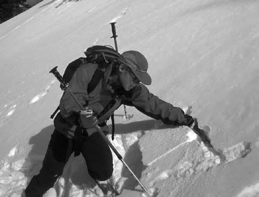
Procedure
1. Place the ski pole perpendicular to the snow surface and push it into the snow (basket end down for soft snow, handle down for harder snow).
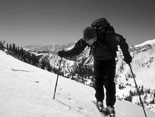
2. Feel for changes in resistance as the ski pole moves through the snowpack.
3. Feel for more subtle layers as the pole is removed from the snowpack by tilting it slightly to the side.
SNOWPACK OBSERVATIONS 43
FIGURE 2.19 A hand shear test. ! Bruce Tremper
FIGURE 2.20 The ski pole poke, aka Ski Pole Penetrometer. ! Bruce Tremper
4. Record the depth, thickness and spatial extent of buried layers.
5. Use other methods to investigate the snowpack as needed.
2.9.7 TILT BOARD TEST
This description follows material published in McClung and Schaerer (2006). The Tilt Board Test is typically used to identify weaknesses in new snow or storm snow layers. The test is gen erally conducted at an established study plot. It can be used to identify weak layers that will be tested with a shear frame.
Equipment
1. Thin metal plate (30 cm x 30 cm).
2. Tilt Board–a board painted white and mounted on a frame. The frame is mounted to a joint that allows it to rotate in the vertical plane. The Tilt Board can be locked in the horizontal position or tilted about 15 degrees. This allows the test block to fracture in shear without sliding off the lower portion of the block.
Procedure
1. Cut a block of snow that is deeper than the suspected weak layer or that contains all of the new or storm snow. McClung and Schaerer (2006) recommend using a block no deeper than 0.4 m.
2. Using a thin metal plate, lift the block on to the Tilt Board.
3. Tap the bottom of the board until the snow fractures.
4. Record your results with the name of the test and rate the result as Easy, Moderate, or Hard (example: Tilt Board Easy or Tilt Board-E).
5. Use other methods to investigate the weak layer or inter face as needed.
2.9.8 SHOVEL TILT TEST
The Shovel Tilt Test is the field worker’s version of the Tilt Board Test but requires no additional equipment be taken into the field. This test can be especially helpful for finding shears within storm snow (Figure 2.21).
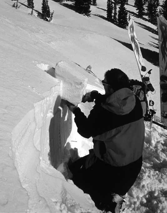
Procedure
1. Isolate a column of snow of similar dimensions to your shovel blade.
2. Insert the shovel blade horizontally into the side of the column below the layers you wish to test (limited to about 0.4 m from the surface).
3. Lift the shovel and snow sample into the air and hold the shovel handle and bottom of the snow column in one hand,
4. Tilt the shovel blade about 5 to 15 degrees steeper than the slope angle of the sample.
5. Tap the bottom of the shovel blade with increasing force until fracture is observed.
6. Record the force required to produce the fracture as Easy, Moderate, or Hard.
7. Shovel tilt may be increased and angle recorded if no frac ture occurs at 15 degrees.
8. Use other methods to investigate the weak layer or inter face as needed.
2.10 INSTRUMENTED METHODS
2.10.1 RAM PENETROMETER Objectives
The Ram Penetrometer is used to obtain a quantifiable measure of the relative hardness or resistance of the snow layers. It can be applied on its own as an index of snow strength, but it is not rec ommended as the sole tool for determining snow stability. When used in combination with a snow profile, a ram profile should be taken about 0.5 m from the pit wall after observation of the snow profile, but before any Shovel Shear Tests are performed. It is a valuable tool for tracking changes in relative hardness over time at study plots and slopes, or for measuring many hardness profiles over an area without digging pits.
The ram profile describes the hardness of layers in the snow pack. However, it often fails to identify thin weak layers in the snowpack, surface hoar layers or other weak layers that are one centimeter or less are difficult to detect. Its sensitivity is depen dent on the hammer weight, particularly when used in soft or very soft snow. The magnitude of this problem may be reduced by using a lightweight hammer (500 g or less), or by using a pow der or “Alta” ram (Perla, 1969).
Refer to Chapter 7 of The Avalanche Handbook (McClung and Schaerer, 2006) for a complete discussion on ram profiles.
44 SNOWPACK
OBSERVATIONS
FIGURE 2.21 The Shovel Tilt Test. ! Howie Garber
Equipment
The standard Ram Penetrometer (Figure 2.22), also called ramsonde, consists of:
• 1 m lead section tube with 40 mm diameter cone and an apex angle of 60°
• Guide rod and anvil
• Hammer of mass 2 kg, 1 kg, 0.5 kg, 0.2 kg or 0.1 kg
• One or two (1.0 m each) extension tubes
The powder ram, also called an Alta Ram (Perla, 1969), consists of:
• 0.50 m to 1.0 m lead section and guide rod and anvil weighing 100 g
• A hammer of mass 0.1 kg
• Lead section cone has the same dimensions as a standard ram
The mass of hammer chosen depends on the expected hard ness of the snow and desired sensitivity.
Unit of Measure
A ram profile depicts the force required to penetrate the snow with a Ram Penetrometer. The mass of the tubes, the mass of the hammer, and the dynamic load of the falling hammer all con tribute to the applied force. Ram profiles can display two differ ent quantities: ram number (RN), which is a mass (kg), and ram resistance (RR), which is a force (N).
Weight is a gravity force that is calculated by multiplying mass by the acceleration due to gravity (9.81 m/s2). Although not strictly correct, most practitioners multiply by 10 to simplify the calculations. Since the ram number is an index of hardness, there is little danger in rounding this value. Force, and consequently the ram resistance, are measured in newtons. A mass of 1 kg has a gravity force (weight) of 1 kg x acceleration which is approxi mately 10 N (1kg x 10m/s2 =10N).
Procedure
Record the location, date, time, observers, slope angle, aspect, and ram type at the head of the data sheet. Also record any notes that will be pertinent to data analysis after leaving the field (Figures 2.23 and 2.24).
Work in pairs if possible. One person holds the Ram Penetrometer in a vertical (plumb) position with the guide rod attached. This person drops the hammer, counts the number of blows, and observes the depth of penetration. The other person records the information. The person holding the ram and drop ping the hammer calls three numbers to the recorder: the drop number, drop height and penetration. For example, “5 from 20 is 143”, means 5 drops from a drop height of 20 cm penetrated to 143 cm (Figure 2.24).
1. Hold the first sectional tube with the guide rod attached directly above the snow surface with the point touching the snow. Let the instrument drop and penetrate the snow under its own weight without slowing it down with your hand. You will need to guide it in many cases so it does not fall over. Record its mass in column T + H. Read the penetration (cm) and record in column p (see Figure 2.24 for field data sheet example). Since the tube weight T is 1.0 kg with the guide rod, it should be attached before the surface measurement is taken. Sometimes a greater
sensitivity of the surface layer is desired. Dropping only the lead section without the guide rod will reduce the weight and may cause less of an initial plunge through the surface layers since the total mass will be lighter. If this method is used, then the weight of the lead section alone should be recorded for the T value, not the combined lead section and guide rod value of 1.0 kg.
2. Carefully add the hammer, or guide rod and hammer if using the lead section only for the surface measurement. Record the mass of the tube + hammer under T + H Read the new penetration and record under p. If the ram does not penetrate further, as is often the case in this step, record the previous p value again.
3. Drop the hammer from a height between 1 cm and 5 cm; record the penetration. The low drop height (1–5 cm) is appropriate for near-surface layers. Larger drop heights (20–60 cm) and increased hammer weights may be desired as depth, and therefore, resistance increases. Continue dropping the hammer from the same height until the rate of penetration changes. Record fall height f, number of blows n, and penetration p up to the point. Some experi ence will allow the user to anticipate changes in the struc ture of the snow and record measurements before the rate of penetration changes. Continue with another series of blows; choose a fall height that produces a penetration of about 1 cm per blow. Do not change fall height or ham mer weight within a series of measurements. Record the series then adjust fall height or change hammer weight if
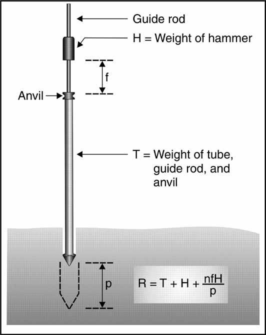
SNOWPACK OBSERVATIONS 45
FIGURE 2.22 Schematic of the Ram Penetrometer (after Perla and Martinelli, 1976).
RAM DATA SHEET
Location: Glory Bowl, Teton Pass, Wilson, WY.
Date: 20220312 Time: 0750 MST
Observer: Newcomb/Elder
Total Depth: 239cm Equipment: Standard Ram Slope: 28° Aspect: 80° Notes: 30m south of GAZEX 1, S3, Wind SW 10m/s
Tube and Hammer Weight T+H (kg)
Number of falls n
Fall height f (cm)
Location of point L (cm)
1 + 0 0 0 23
Comments
Tube and guide rod only, new snow deposited last 18 hr
1 + 0.5 0 0 25 add 0.5kg hammer no drop 6 1 32
1 + 1 0 0 32 change to 1kg hammer 4 5 37 11 10 49 7 20 52 crust 5 10 64 15 10 87
2 + 1 0 0 87 add 2nd tube section 10 20 108 13 30 141 6 30 148 3 + 1 0 0 148 add 3rd tube section 25 30 181 22 30 209 1 30 215 3 10 239
FIGURE 2.23 Sample field book page for ram profiles.
RAM CALCULATION SHEET
Location: Glory Bowl, Teton Pass, Wilson, WY Date: 20220312 Time: 0750 MST
Observer: Newcomb/Elder Total Depth: 239cm Equipment: Standard Ram Slope: 28° Aspect: 80°
Number of falls n
Fall height f (cm)
Location of point L (cm)
RN = T + H + (nfH)/p (kg)Notes: 30m south of GAZEX 1, S3 Wind SW 10m/s RR = RN x 10 (N) Tube and Hammer Weight T+H (kg)
Penetration p (cm) (nfH)/p (kg) RN (kg) RR (N) Height above ground (cm) 239
1 + 0 0 0 23 23 0.0 1.0 10 216 1 + 0.5 0 0 25 2 0.0 1.5 15 214 6 1 32 7 0.4 1.9 19 207 1 + 1 0 0 32 0 207 4 5 37 5 4.0 6.0 60 202 11 10 49 12 9.2 11.2 112 190 7 20 52 3 46.7 48.7 487 187 5 10 64 12 4.2 6.2 62 175 15 10 87 23 6.5 8.5 85 152 2 + 1 0 0 87 0 152 10 20 108 21 9.5 12.5 125 131 13 30 141 33 11.8 14.8 148 98 6 30 148 7 25.7 28.7 287 91 3 + 1 0 0 148 0 91 25 30 181 33 22.7 26.6 266 58 22 30 209 28 23.6 27.6 276 30 1 30 215 6 5.0 9.0 90 24 3 10 239 24 1.3 5.3 53 0
FIGURE 2.24 Sample worksheet page for calculating ram profiles.
46 SNOWPACK OBSERVATIONS
desired before beginning another series. Resolution of the profile depends on the frequency of recorded measure ments and the snowpack structure. Many recorded mea surements in a homogeneous layer will provide no more resolution than fewer measurements since the calculated RN will be the same for both. However, resolution will be lost in varied layers if too many drops are made between recordings as the layer will receive a single RN over the entire range of p for that layer.
4. Add another section of tube when necessary and record the new T + H.
5. Repeat the measurements (b and c) until the ground sur face is reached.
Calculation
1. Calculate the increment of penetration p for each series of blows by subtracting the previous p value from the pres ent p value (Figure 2.25).
2. Calculate ram number (RN) or ram resistance (RR) with the following equations:
RN=T + H+ nfH ⍴ RR = RN x 10
where:
RN = ram number (kg) RR = ram resistance (N) n = number of blows of the hammer f = fall height of the hammer (cm) p = increment of penetration for n blows (cm) T = mass of tubes including guide rod (kg) H = mass of hammer (kg)
3. Plot on graph paper the ram number or resistance vs. depth of snow (see Figure 2.25).
2.10.2 SHEAR FRAME TEST
The Shear Frame Test is used to measure the shear strength of snow layers and interfaces between snow layers (Figure 2.26).
The Shear Frame Test requires experience but provides use ful information when done correctly and consistently. The test combined with a stability ratio is a useful tool for assessing the strength of snow layers. Discussions of shear frame methods can be found in Jamieson, 2001; Jamieson, 1995; Fohn, 1987b, Perla and Beck, 1983, and Roch, 1966.
Equipment
The Shear Frame Test requires the following equipment:
1. Putty knife
2. Metal cutting plate about 30 cm x 30 cm
3. Shear frame, usually 100 cm2 or 250 cm2
4. Force gauge, maximum capacity 10 to 250 N (1 to 25 kg).
If you are calculating the stability ratio, you will also need the following equipment:
5. Sampling tube, 50 to 80 cm
6. Weighing scale
FIGURE 2.25 Graphical representation of a ram profile from data listed in Figures 2.23 and 2.24.

Procedure
The Shear Frame Test can be performed on storm snow layers and persistent weak layers. Typically 100 cm2 frames are used for storm snow layers and 250 cm2 are used for persistent weak layers.
Observers generally perform 7 to 12 consecutive tests and average the results. Once a series of measurements is started it is important to not switch frame sizes.
1. Identify weak layer using tilt board or other method.
2. Remove the overlying snow to within 4 or 5 cm of the layer or interface being measured.
3. Carefully insert the shear frame into the snow so the bot tom of the frame is 2 to 5 mm above the layer.
4. Pass a thin blade (putty knife) around the shear frame to remove snow that was in contact with the frame.
5. Attach an appropriate force gauge and pull so that frac ture occurs within 1 second. This method ensures brittle fracture. It is essential that the operator loads the force gauge at a constant rate and is consistent between all measurements.
Shear Strength Calculation
Once you have obtained the average shear force for the weak layer or interface, calculate the shear strength from the formula: F average A average
Tframe =
where F average is the average shear force in newtons (N), Aframe is the area of the shear frame in m2, and Tframe is the shear strength of the layer in pascals (Pa). This calculation produces a shear strength that is dependent on the shear frame size (Tframe= T 250 or T100). For
SNOWPACK OBSERVATIONS 47
FIGURE 2.26 Measuring shear strength with a shear frame.
a value of shear strength that is independent of frame size use the following equations (Föhn, 1987b; Jamieson, 1995):
T ∞ = 0.65T 250 T ∞ = 0.56 T 100
where T ∞ is the shear strength independent of shear frame size and T 250 and T 100 are the shear strengths measured with a 250 cm2 and 100 cm2 shear frame respectively.
Stability Ratios
The stability ratio is the shear strength of a layer divided by the overlying slab’s weight per unit area. The stability ratio has a complex relationship with avalanche occurrence, but in general the lower the ratio the greater the likelihood of avalanches.
shear strength weight per unit areaStability Ratio (SR) =
To determine the slab’s weight per unit area, slide a small plate such as a putty knife or crystal card horizontally into the pit wall at a depth equal to the sampling tube length. Now slide the sam pling tube vertically down through the surface until it strikes the plate. Excavate the sampling tube, taking care not to lose any snow out of the end of the tube. Transfer the contents of the sampling tube to a plastic bag for weighing. Divide the sample weight by the cross sectional area of the tube to calculate the slab weight per unit area. For weak layers deeper than the sampling tube length, use a stepped sampling method.

Results
The shear frame works best for thin weak layers or storm snow interfaces. Thick weak layers (i.e. depth hoar) tend not to pro duce consistent fracture planes. The shear frame works poorly in situations where very hard layers (i.e. wind slabs and crusts) are directly above weak layers. The problem is inserting the shear frame into the hard layer without fracturing the weak layer below. In addition, there is little operational experience and liter ature on the use of shear frames with wet snow. The shear frame is sensitive to user variability.
Shear Frame References
Föhn, P.M.B., 1987: The stability index and various triggering mechanisms. Avalanche Formation, Movement, and Effects, In: B. Salm and H. Gubler, (eds.), IAHS-AISH Publication No. 162, 195–211.
Jamieson, J.B., 1995: Avalanche prediction for persistent snow slabs, Ph.D. dissertation, University of Calgary, Alberta. 53–58. Jamieson, J.B., and C.D. Johnston, 2001: Evaluation of the Shear Frame Test for weak snowpack layers. Annals of Glaciology, 32, 59–66.
Perla, R.I., and T.M.K. Beck, 1983: Experience with shear frames. Journal of Glaciology, 29, 485–491.
Roch, A., 1966: Les variations de la resistence de la neige. Proceedings of the International Symposium on Scientific aspects of Snow and Ice Avalanches. Gentbrugge, Belgium, IAHS Publication, 182–195.
48 SNOWPACK OBSERVATIONS
AVALANCHE OBSERVATIONS
3.1 INTRODUCTION
Observations of past and present avalanche activity are of the utmost importance for any avalanche forecasting operation. These data should be recorded and organized in a manner that allows personnel to visualize temporal and spatial patterns in recent avalanche activity. Objectives for observing avalanches are presented in Section 3.2. A standard avalanche observation is presented in Section 3.4. The remainder of this chapter pro vides methods for observing a wide variety of avalanche related phenomena. Parameters are divided into avalanche path charac teristics and avalanche event characteristics. Parameters in the standard avalanche observation are marked with a symbol.
Individual operations can choose to observe and record parameters beyond those included in the standard observation. The parameters collected will depend on the type of operation and the snow climate of the forecast area.
3.2 OBJECTIVES
Observations and records of avalanche occurrences have the fol lowing applications:
• Information about avalanche occurrences and non-oc currences is used in association with other observations in evaluating snow stability.
• Observations identify areas where avalanches released earlier in the winter or storm/avalanche cycle. Snow sta bility may vary between these sites and nearby undis turbed slopes.
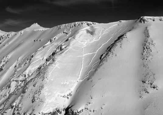
• Avalanche observation data are essential when protective works and facilities are planned, when the effectiveness of mitigation measures is assessed, and when forecasting models are developed by correlating past weather and snow conditions with avalanche occurrences.
• Understanding the avalanche phenomenon through research.
All avalanches that are significant to an operation should be recorded. Noting the non-occurrence of avalanches is also important for snow stability evaluation and during hazard reduction missions.
3.3 IDENTIFICATION OF AVALANCHE PATHS
Avalanche paths should be identified by a key name, number, aspect, or a similar identifier which should be referred to on lists, maps, or photographs. For roads, railway lines, and power lines it is convenient to refer to avalanche paths by the running mile or kilometer. Every effort should be made to retain histori cal names. Changing historical names creates confusing records and decreases the usefulness of past data records. Historical paths that have multiple starting zones can be reclassified with subcategories of the original name. Any reclassification should be clearly explained in the metadata (see Appendix C).
Avalanche paths with multiple starting zones are often divided into sub-zones. Separate targets for explosive placement may be identified within each starting zone (Figure 3.1).
3.4 STANDARD AVALANCHE OBSERVATION
This section outlines a standard avalanche observation for singleavalanche events. Suggestions for summarizing multiple ava lanche events are discussed in Section 3.7. Storm cycles and access to starting zones may make it difficult to observe every parameter for every avalanche that occurs within a forecast area. In this case the avalanche size characteristics should be esti mated, and some of the snow specific parameters can be marked N/O for "not observed."
The parameters have been separated into avalanche path char acteristics and avalanche event characteristics. Operations that deal with a “fixed” number of paths documented in an avalanche atlas replace the path specific parameters with path name or number.
1. Date — Record the date on which the avalanche occurred (YYYYMMDD).
2. Time — Record the standard local time the avalanche occurred to the hour or minute if possible. Time codes of 2405 and 2417 can be used for avalanches that released at an unknown time during the AM and PM respectively. Time ranges or start and end times of mitigation missions can also be used.
3. Observer — Record the name or names of the personnel that made the observation.
4. Path Characteristics (Section 3.5)
a. Observation Location — Record the name or number of the path where the avalanche occurred, the latitude and longitude, or the nearest prominent topographic landmark (mountain, pass, drainage, etc.) or political landmark (town, road mile, etc.).
b. Aspect — Record the direction the slope faces where the avalanche occurred (N, NE, E, SE, S, SW, W, NW).
c. Slope Angle in Starting Zone — Record the average slope angle in the starting zone where the avalanche released. When possible, a number of locations in the starting zone should be measured so that a maximum, minimum, and average value can be reported.
d. Elevation — Record the elevation of the crown face in feet (meters).
49
FIGURE 3.1 Explosive triggered slab avalanche. ! Matt Steen
5. Event Characteristics (Section
3.6)
a. Type — Record the avalanche type.
b. Trigger — Record the event that triggered the avalanche.
c. Size — Record the size of the avalanche.
d. Snow Properties
i. Bed Surface — Record the location of the bed sur face as one of the following: in new snow (S), at the new/old interface (I), in old snow (O), or at the ground (G). If the site was visited, record the hand hardness, grain type, and grain size.
ii. Weak Layer — Record the grain type and date of burial if known. If the site was visited record the hand hardness, grain type, and grain size.
iii. Slab — Record the hand hardness, grain type, and grain size.
e. Dimensions
i. Slab Thickness — Record the average and maxi mum thickness or height of the crown face to the nearest 0.25 m (or whole foot).
ii. Width — Record the width (horizontal distance) of the avalanche to the nearest 10 m (or 25 ft).
iii. Vertical Fall — Record the vertical fall of the ava lanche to the nearest 30 m (or 100 ft).
f. Location of Start Zone — Record the location of the crown face, as viewed from below, within the starting zone as top (T), middle (M), or bottom (B).
g. Terminus — Record the location of the debris within the avalanche path.
3.5 AVALANCHE PATH CHARACTERISTICS
3.5.1 AREA AND PATH
Enter the name of the operation or avalanche area where the ava lanche path is located (Table 3.1). Enter the identifier (name or number) of the avalanche path. Some road operations may name their paths by the running mile or kilometer. In this case two dec imal places may be used to identify paths within a whole mile or kilometer.
3.5.2 ASPECT
Use the eight points of the compass to specify the avalanche’s central aspect in the starting zone. Compass degrees or the six teen major points (i.e. NNE, ENE, etc.) may be used to convey greater detail. A range in aspect can be specified for large or highly curved starting zones.
TABLE 3.1 Slope Aspect
3.5.3 SLOPE ANGLE
Record the average slope angle (to the nearest whole degree) in the starting zone where the avalanche released. When possible, a number of locations in the starting zone should be measured so that a maximum, minimum and average value can be reported (Figure 3.2).
FIGURE 3.2 Measuring the slope angle of a slab avalanche. ! Bruce Tremper
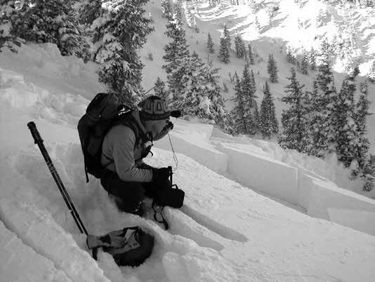
3.5.4
ELEVATION
Record the elevation of the starting zone or crown face in feet (or meters) above sea level (ASL).
3.6 AVALANCHE EVENT CHARACTERISTICS
3.6.1 DATE
Record year, month and day of the avalanche occurrence (avoid spaces, commas, etc.); i.e. December 15, 2023, is noted as 20231215 (YYYYMMDD).
3.6.2 TIME
Estimate the time of occurrence and record it by hour and min ute in local standard time.
Record the time of occurrence on the 24-hour clock (avoid spaces, colons, etc.); i.e. 5:10 p.m. is noted as 1710.
Use local standard time (i.e. Pacific, Mountain, etc.). Operations that overlap time zones should standardize to one time.
50 AVALANCHE
OBSERVATIONS
N NE E SE S SW W NW
0 45 90 135 180 225 270 315
DIRECTION
DEGREES
TABLE
Avalanche Type DATA CODE TYPE L Loose-snow avalanche WL Wet loose-snow avalanche SS Soft slab avalanche HS Hard slab avalanche WS Wet slab avalanche I Ice fall or avalanche SF Slush flow C Cornice fall (w/o additional avalanche) R Roof avalanche U Unknown
3.2
When the precise time of occurrence is unknown, use 2405 and 2417 for avalanches that released during the AM and PM respectively. Time ranges or start and end times of mitigation missions can also be used.
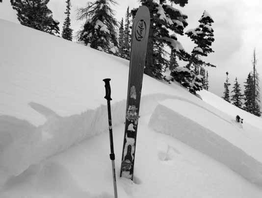
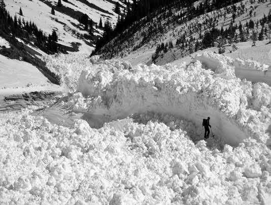
3.6.3 AVALANCHE TYPE
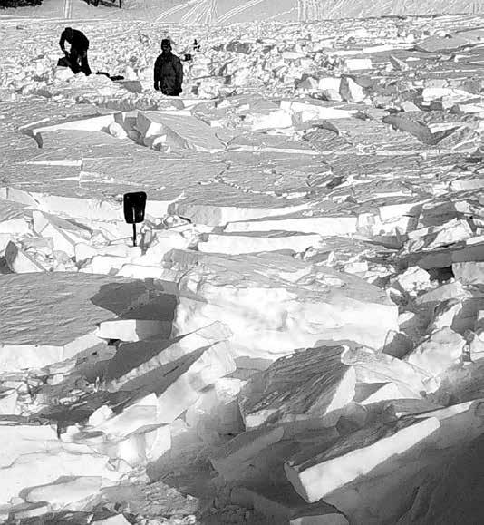
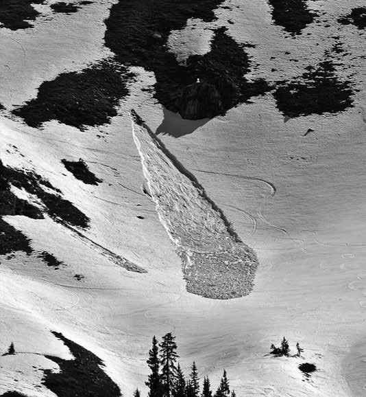
Record the type of avalanche as described in Table 3.2. A hard slab has an average density equal to or greater than 300 kg/m3. Informal distinctions can be made between hard and soft slab avalanches based on the form of the deposit and the hand hardness of the slab. Hard slab avalanches generally have a slab hardness of one finger or greater. Debris piles from hard slab ava lanches are typically composed of angular blocks of snow.
3.6.4 TRIGGER
Indicate the mechanism that caused the avalanche with a primary
code, secondary code when possible, and modifier when appro priate. The secondary codes have been separated into two catego ries with separate modifiers for each. Operations may devise other trigger sub-classes that apply to their specific conditions in con sultation with the American Avalanche Association. Guidelines for reporting avalanche involvements are listed in Appendix H. Examples of coding structure are given in Section 3.6.12.
AVALANCHE OBSERVATIONS 51
FIGURE 3.3 Avalanche types clockwise from top-left: soft slab avalanche; wet debris; debris from a hard slab avalanche; point release avalanche or sluff.
! Bruce Tremper, Matt Steen, Karl Birkeland, and Colorado Avalanche Information Center
DATA CODE
RELEASE N Natural or Spontaneous A Artificial U Unknown
TABLE 3.3 Avalanche Trigger Codes — Primary
CAUSE OF AVALANCHE
TABLE 3.4 Avalanche Trigger Codes — Secondary — Human, Vehicle,and Miscellaneous Artificially Triggered Releases
DATA CODE CAUSE OF AVALANCHE RELEASE
ARTIFICIAL TRIGGERS: VEHICLE
AM Snowmobile
AN Motorized Snowbike
AK Snowcat
AV Vehicle (specify in comments)
ARTIFICIAL TRIGGERS: HUMAN
AS Skier
AR Snowboarder
AI Snowshoer
AF Foot penetration
AC Cornice fall produced by human or explosive action
ARTIFICIAL TRIGGERS: MISCELLANEOUS
AU Unknown artificial trigger
AO
Unclassified artificial trigger (specify in comments)
TABLE 3.6 Avalanche Trigger Codes — Secondary — Natural and Explosively Triggered Releases
DATA CODE CAUSE OF AVALANCHE RELEASE
NATURAL OR SPONTANEOUS
N Natural trigger NC Cornice fall NE Earthquake
NI Ice fall NL
Avalanche triggered by loose snow ava lanche (Figure 3.4)
NS Avalanche triggered by slab avalanche NR Rock fall NO
Unclassified natural trigger (specify in comments)
ARTIFICIAL TRIGGERS: EXPLOSIVE
AA Artillery
TABLE 3.5 Avalanche Trigger Code Modifiers for Human, Vehicle, and Miscellaneous Artificially Triggered Releases
DATA CODE CAUSE OF AVALANCHE RELEASE
c
An intentional release by the indicated trigger (i.e. slope cut, intentional cor nice drop, etc.)
u An unintentional release
r A remote avalanche released by the indicated trigger
y An avalanche released in sympathy with another avalanche
An explosive thrown or placed on or under the snow surface by hand AL Avalauncher
AE
AB An explosive detonated above the snow surface (air blast)
AC Cornice fall triggered by human or explosive action
AX Gas exploder
AH Explosives placed via helicopter
AP Pre-placed on or in the snow, remotely detonated explosive charge
ARTIFICIAL TRIGGERS: MISCELLANEOUS
AW Wild or Domesticated Animal
AU Unknown artificial trigger
AO
TABLE 3.7 Avalanche Trigger Code Modifiers for Natural and Explosively Triggered Releases
DATA CODE CAUSE OF AVALANCHE RELEASE
r
A remote avalanche released by the indicated trigger
y An avalanche released in sympathy with another avalanche
Unclassified artificial trigger (specify in comments)
Note for Table 3.7: For remote and sympathetic avalanches the distance between the trigger and the avalanche should be recorded in the comments.
Avalanches that start when a helicopter or other aircraft flies overhead should be considered natural if the aircraft is a significant distance (out of ground effect) above the ground.
Avalanches triggered by a helicopter when it is touching the snow should be recorded as AV. Avalanches triggered by a helicopter in “ground effect” should be recorded as AVr. Use your best judgment.
52 AVALANCHE OBSERVATIONS
DATA CODE AVALANCHE DESTRUCTIVE POTENTIAL TYPICAL MASS TYPICAL PATH LENGTH TYPICAL IMPACT PRESSURE
D1 Relatively harmless to people.
<10 t 10 m 1 kPa
D2 Could bury, injure, or kill a person. 102 t 100 m 10 kPa
D3 Could bury and destroy a car, dam age a truck, destroy a wood frame house, or break a few trees. 103 t 1000 m 100 kPa
D4 Could destroy a railway car, large truck, several buildings, or substan tial amount of forest. 104 t 2000 m 500 kPa
D5 Could gouge the landscape. Larg est snow avalanche known. 105 t 3000 m 1,000 kPa
Note for Table 3.8: Half-sizes may be used to signify an avalanche that is on the high end of a single class.
The destructive potential of avalanches is a function of their mass, speed and density as well as the length and cross-section of the avalanche path.
Typical impact pressures for each size number are given in McClung and Schaerer (1981). The number “0” may be used to indicate no release of an avalanche following the application of mitigation measures.
3.6.5 SIZE
The two commonly used avalanche size classification schemes are: 1) destructive force, and 2) relative to path. Both systems use a scale that varies from 1 to 5. These guidelines recommend observing and recording avalanche size in both systems. Using both systems will maintain long-term data sets and provide the most useful information to active forecasting programs. However, forecasting program managers should decide whether to use one or both schemes. Each system provides different and useful infor mation, but the numerical categories of each scale are often not comparable.
3.6.5.1 SIZE — DESTRUCTIVE FORCE
Estimate the destructive potential of the avalanche from the mass of deposited snow, and assign a size number. Imagine that the objects described in Table 3.8 (people, cars, trees, etc.) were located in the track or at the beginning of the runout zone and estimate the harm the avalanche would have caused.
3.6.5.2 SIZE — RELATIVE TO PATH
The size relative to path classification is a general measure and takes into account many factors, including the horizontal extent and vertical depth of the fracture, the volume and mass of the debris, and the runout distance of the avalanche. The observer estimates the size of the avalanche relative to the terrain fea ture or avalanche path where it occurred. A “small” avalanche is one that is relatively small compared to what that particular avalanche path could produce, while a “large” avalanche is, or is close to, the largest avalanche that the particular avalanche path could produce.
Determining the relative size of an avalanche requires com paring the observed event to an estimate of the smallest and larg est avalanches that path could produce. The R-size is not simply the proportion of the start zone that released. Rather, R-sizes account for the depth, width, and length of the slab, the amount of snow entrained in the track, and the snow conditions in the track and runout.
TABLE 3.9 Avalanche Size — Relative to Path
DATA CODE AVALANCHE SIZE
Very small, relative to the path
Small, relative to the path
Medium, relative to the path
Large, relative to the path R5 Major or maximum, relative to the path
Note for Table 3.9: Half-sizes should not be used for the SizeRelative to Path scale.
The number “0” may be used to indicate no release of an ava lanche following the application of mitigation measures.
The size classification pertains to both the horizontal extent and the vertical depth of the fracture, as well as the volume and runout distance of the avalanche.
AVALANCHE OBSERVATIONS 53
TABLE 3.8 Avalanche Size —
Destructive Force (after CAA, 2007; Perla, 1980)
R1
R2
R3
R4
3.6.6 SNOW PROPERTIES
3.6.6.1 BED SURFACE
Level of Bed Surface
Record the level of the bed surface (the upper surface of the layer over which a slab slid) in the snowpack per Table 3.10. If the ava lanche involved more than one bed surface, all applicable codes should be included.
TABLE 3.10 Avalanche Bed Surface
DATA CODE BED SURFACE
Form and Age of Fracture Plane
Record the predominant grain form observed in the layer below the fracture plane using the International Classification for Seasonal Snow on the Ground (refer to Appendix F). Where pos sible identify the failure plane by its probable date of burial. Use the comments section to note the occurrence of a fracture that steps down to other layers.
3.6.6.2 WEAK LAYER
Record the grain type using the International Classification for Seasonal Snow on the Ground (see Appendix F), grain size (mm), and hand hardness of the weak layer.
3.6.6.3 SLAB
Record the grain type using the International Classification for Seasonal Snow on the Ground (see Appendix F), grain size (mm), and hand hardness of the slab directly above the weak layer.
3.6.6.4 LIQUID WATER CONTENT IN STARTING ZONE AND DEPOSIT
Determine the liquid water content of the avalanche snow in the starting zone and deposit at the time of failure and deposition. The liquid water content can be different in the starting zone and deposit.
Although start zone and deposit observations use the same data code, they can be recorded as two separate items to include more information.
TABLE 3.11 Liquid Water Content of Snow in Avalanche Starting Zone
DATA CODE LIQUID WATER CONTENT
D Dry snow M Moist snow W Wet snow U Unknown
Note: See Table 2.4 for water content definitions.
3.6.7 AVALANCHE DIMENSIONS
S
The avalanche released within a layer of recent storm snow. I
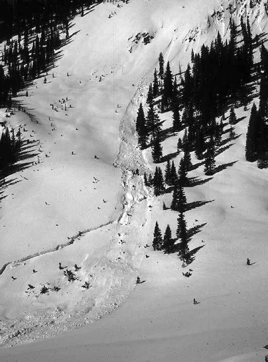
The avalanche released at the new snow/old snow interface. O
The avalanche released within the old snow. G
The avalanche released at the ground, glacial ice or firn. U Unknown
Note for Table 3.10: Storm snow is defined here as all snow deposited during a recent storm.
The dimensions of an avalanche can be measured in the field, or by using digital methods. Whenever possible, include a descrip tion of how you determined each value (tools, methods, sources of error, etc.).
3.6.7.1 SLAB THICKNESS
If practical, estimate or measure the average and maximum thickness of the slab (normal to the slope to the nearest 25 cen timeters or whole foot) and the average thickness of the slab at the fracture line. If only one value is reported it should be the average dimension. Add “M” when the slab is actually measured.
3.6.7.2 SLAB WIDTH
In a slab avalanche, record the width (horizontal distance) in meters (feet) of the slab between the flanks near the fracture line. Add “M” when width is actually measured.
54 AVALANCHE OBSERVATIONS
FIGURE 3.4 Slab avalanche triggered by a loose-snow avalanche.
! Andy Gleason
FIGURE 3.5 Slab avalanches remotely triggered by foot penetration. ! John Sykes
3.6.7.3
VERTICAL FALL
Using an altimeter or contour map, calculate the elevation dif ference in feet (meters) between the fracture line and the toe of the debris.
3.6.7.4
LENGTH OF PATH RUN
Some operations may wish to record the estimated distance an ava lanche ran along a slope. Record the distance between the fracture line and the toe of the debris. Up to a distance of 300 m (~ 1000 ft) estimate the distance traveled to the nearest 25 m (~ 100 ft). Beyond a distance of 300 m estimate the distance traveled to the nearest 100 m (~ 300 ft). All dimensions are assumed to be estimates unless the values are followed with the letter M (measured). Dimensions are assumed to be in meters. Measurements or estimates in feet should be indicated with a ' after the number (i.e. 3').
3.6.8 LOCATION OF AVALANCHE START
Position in Starting Zone
Describe the location of the avalanche fracture with one of the following code letters, physical features or elevation and, when applicable, add the data code for the starting sub-zone or the target.
Note: For this code (Table 3.12) gunner’s left and right should be used. Gunner’s perspective is looking up at the starting zone (oppo site of skier’s perspective).
TABLE 3.12 Location of Avalanche Start DATA CODE
VERTICAL LOCATION WITHIN STARTING ZONE FROM GUNNER'S PERSPECTIVE
T (L, R, C)
At the top of the starting zone (left, right, or center)
M (L, R, C) In the middle of the starting zone (left, right, or center)
B (L, R, C) At the bottom of the starting zone (left, right, or center)
U Unknown
Note for Tables 3.12 and 3.13: The codes TP, MP and BP are appli cable for short paths where the starting zone, track and runout zone cannot be easily separated.
3.6.9
TERMINUS
Describe the location of the toe of the avalanche deposit with a data code. See Table 3.13.
3.6.10
TOTAL DEPOSIT DIMENSIONS
Record the average width and length of the deposited avalanche snow in meters (feet).
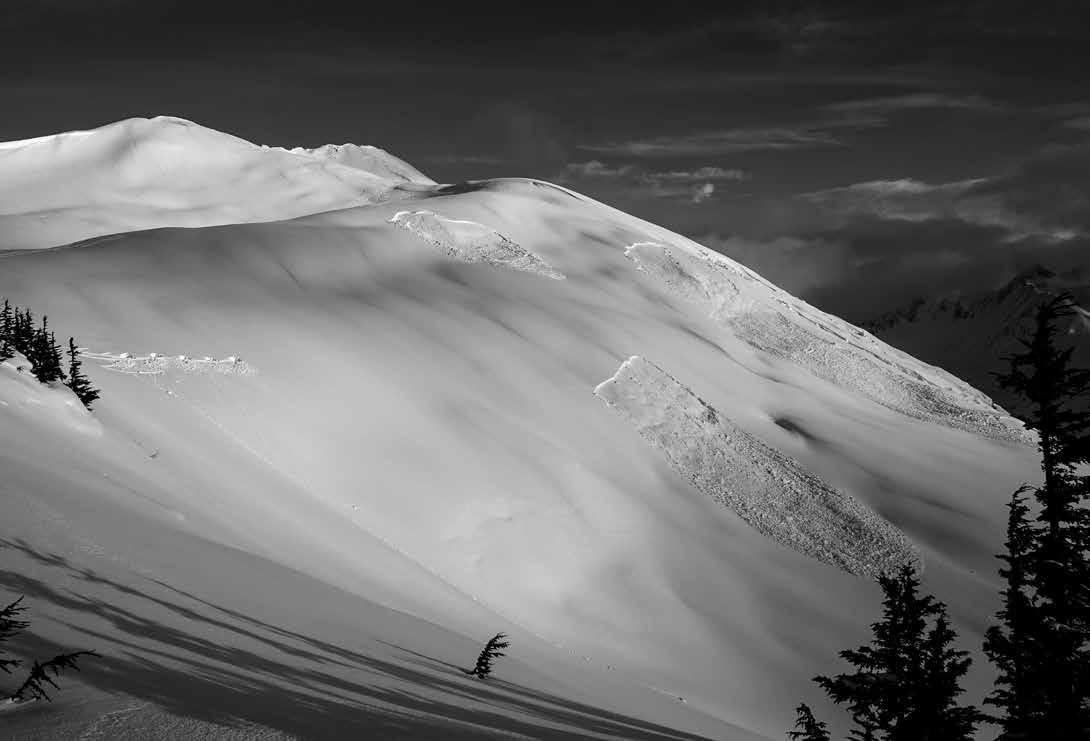
AVALANCHE OBSERVATIONS 55
TABLE
3.13
Terminus of Avalanche Debris
DATA CODE TERMINUS FOR LONG PATHS
SZ The avalanche stopped in the starting zone
TK The avalanche stopped in the track
TR The avalanche stopped at the top part of the runout zone
MR The avalanche stopped in the middle part of the runout zone
BR The avalanche stopped in the bottom part of the runout zone
U Unknown
DATA
CODE TERMINUS FOR SHORT PATHS
TP The avalanche stopped near the top of the path
MP The avalanche stopped near the middle part of the path
BP The avalanche stopped near the bot tom part of the path
Note: Operations that have large avalanche paths with welldefined features may apply additional codes (See Table 3.14).
Record the average deposit depth in meters and tenths of a meter. Add an “M” after each value if measured by tape or probe.
3.6.11 AVALANCHE RUNOUT
The angle between the horizontal and a line drawn from the highest portion of the crown face and the toe of the debris can be used as a relative measure of avalanche runout. This angle, known as the runout angle or alpha angle (α), has been used by landslide investigators since the late 1800s and has been applied to ava lanche studies to describe extreme (~100 year) events. Although α is often used for very large events in avalanche research, guide services, engineers, scientists, and forecasters may also find the subcategories defined in Table 3.15 useful. The runout angle can be calculated with the following equation where h is the verti cal height and l is the horizontal distance, both should be deter mined from the highest point of the crown face to the farthest reach of the deposit.
α = =( )h l ( )h l arctan tan-1
Statistical studies suggest that alpha angles in a specific mountain range can cluster around a characteristic value. This value may be governed by terrain and snowpack condi tions characteristic of the range (McClung and Schaerer, 2006; Mears, 1992; McClung and others, 1989; Lied and Bakkehøi, 1980).
TABLE 3.14 Detailed Terminus Codes
DATA CODE TERMINUS
1F Stopped on top ¼ of the fan
2F Stopped halfway down the fan
3F Stopped ¾ of way down the fan
TABLE
3.15 Alpha Angle Subcategories
DATA CODE DESCRIPTION
The measured alpha angle for any indi vidual avalanche. α e
α
The alpha angle of an extreme event. The smallest alpha angle (furthest av alanche runout) observed in a specific avalanche path, determined by histori cal records, tree ring analysis, or direct observation.
α number
A calculated value of the smallest alpha angle (furthest avalanche runout) in a specific avalanche path during a de fined time period. Where the designat ed time period (return period) in years is listed in the subscript (α10, α50, α100).
3.6.12 CODING AVALANCHE OBSERVATIONS
Avalanche observations can be recorded in tabular format with a separate column for each data code. Common data codes can also be recorded in one string.
Example:
HS-AA-R2-D2: a hard slab avalanche triggered artificially by artillery SS-AE-R4-D3: a soft slab avalanche triggered artificially by a hand charge L-N-R1-D1: a small loose snow avalanche that released naturally HS-ASr-R3-D3-O: a hard slab avalanche triggered remotely by a skier that broke into old snow layers (see Section 3.6.4) HS-ACu-R4-D3: a hard slab avalanche triggered by an unintentional artificial cornice fall HS-ACc-R2-D3: a hard slab avalanche triggered by an intentional artificial cornice fall HS-AC-R2-D3: a hard slab avalanche triggered by a cornice drop produced by explosives WS-NS-R4-D3: a wet slab triggered by a natural slab avalanche. AC-0: An intentionally triggered cornice that did not pro duce an avalanche
3.6.13 COMMENTS
Enter information about damage and accidents caused by the avalanche and any other significant information. Note when the avalanche was triggered artificially. Use as much space as required.
56 AVALANCHE OBSERVATIONS
Multiple Avalanche Events — Recording Example
PARAMETER CRITERIA EXAMPLES
Date or date range
Record beginning of cycle and end of cycle when possible 20220212 or 20220212–20220214
Time range Digits 0000–1000
Area (location) Text (80 characters max.) Mt. Timpanogos
Size Attempt to limit the size range to 2 classes. Significant or very large avalanches should be recorded as individ ual events D1.5–D2.0 R2-R3
Trigger
Trigger Data code (do not mix natural and artificial trig gers in this report) AE, U
Type Data code (group slab and loose avalanches separately) HS, SS, U, or WL, U
Aspect (of starting zone) A single, range, or a combination of compass directions All, W, SW–NW
Elevation (at fracture)
Slope Angle (at fracture)
Group events by elevation range. Use separate reports for significant elevation ranges as applicable to forecast area 5000–6500 and 8000–10,000 ft.
Record range in average starting zone angle and min and max 32–42, 30, 45
Level of bed surface Key letter (do not mix storm snow, old snow, and ground) S, O, G, or U
Hardness of bed surface Hand hardness scale 1F
Weak layer grain form Grain abbreviation (Fierz et al., 2009) SH
Hardness of weak layer Hand hardness scale 4F
Age of failure plane Probable date of burial 20220204
Slab width Range (in meters) 60–110 m
Slab thickness Range (in centimeters) 10–30 cm
Hardness of slab Hand hardness scale P
Vertical fall
Comments
Range (in meters) 500–1500 m
Max. of 5 lines by 80 characters per line
3.7 MULTIPLE AVALANCHE EVENTS
An operation may wish to group large numbers of similar ava lanche events (avalanche cycle) into one record or report, espe cially if that information is to be sent to a central information exchange. Grouping is achieved by allowing certain fields to hold a range of values (i.e. by specifying lower and upper bounds, sepa rated by a dash). The report should be repeated for different types of activity (i.e. natural versus artificially released avalanches).
Significant avalanches (larger than size D3 or R3), and events involving incident, damage or injury should be described individually.
3.8 ADDITIONAL OBSERVATIONS
Additional observations may be selected as applicable from those listed in this section. Certain additional observations are valuable in areas where avalanches are either mitigated or affect traffic and/or communication lines.
3.8.1 AVALANCHE HAZARD MITIGATION MISSIONS
3.8.1.1 NUMBER OF EXPLOSIVE CHARGES / NUMBER OF DETONATIONS
Record the number of projectiles or explosive charges applied to a target. Record the number of confirmed detonations. The difference in the two values gives a dud count.
AVALANCHE OBSERVATIONS 57
TABLE 3.16
3.8.1.2 SIZE OF EXPLOSIVE CHARGE
Note the mass (kg) of the explosive charge used at each shot location.
3.8.2 ROAD AND RAILWAY OPERATIONS
3.8.2.1
DEPOSIT ON ROAD OR RAILWAY
Record in meters (feet) the length of road, railway line, ski run, power line, or other facility buried in avalanche debris.
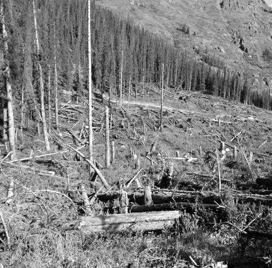
Record average depth at center line and maximum depth of ava lanche debris on the road, etc., in meters and tenths of a meter (feet/inches). Add “M” when length and depth are measured.
3.8.2.2 TOE MASS DISTANCE
Measure or estimate the distance between the uphill edge of the road, or other development, and the farthest point reached by the mass of avalanche. Negative values are used when the deposited mass failed to reach the road or facility. Some operations may also wish to document the occurrence of snow dust on the road. Dust results from the fallout of an avalanche’s powder cloud. Its main impact is on driver visibility.
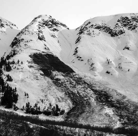
3.8.2.3
ROAD / LINE STATUS
Transportation operations should record the status (open or closed) and danger rating (Appendix G) in effect for any roads or railway lines at the time when the avalanche occurred. During closures due to mitigation missions or avalanche activity, the start and end time of the closure should be recorded.
58 AVALANCHE OBSERVATIONS
FIGURE 3.6 An avalanche triggered by glide of the snowpack. ! Heather Thamm
FIGURE 3.7 Trees damaged in the runout zone of a large avalanche path. ! Ethan Greene
GLOSSARY
Accuracy — The difference between the measured value and the actual or true value. A property of a measurement method and instruments used. Also see precision
Alpha Angle —The angle between the horizontal and a line drawn from the highest point of the crown face to the toe of the debris. Alpha can be measured for an individual avalanche (α ). Extreme values of alpha (α e) can be determined from his torical records, tree ring data, or direct observation. Minimum values of alpha (longest runout length) can also be estimated for a specific return period (α10, α50, α 100). Also termed runout angle or angle of reach
Anemometer — An instrument that measures the pressure exerted by, or the speed of, wind.
Aspect — The exposure of the terrain as indicated by compass direction of the fall line (relative to true north). A slope that faces north has a north aspect.
Atmospheric Pressure — The pressure due to the weight of air on the surface of the earth or at a given level in the atmosphere. Also called barometric pressure.
Avalanche, Snow — A mass of snow sliding, tumbling, or flow ing down an inclined surface that may contain rocks, soil, veg etation, or ice.
Avalanche Danger Scale — A categorical estimation of the ava lanche danger. In the U.S., a five-level scale is used for back country recreational users. See Appendix G.
Avalanche Path — A terrain feature where an avalanche occurs. An avalanche path is composed of a starting zone, track, and runout zone.
Avalauncher — A compressed gas delivery system for explo sives. Designed for avalanche hazard mitigation.
Barometer — An instrument that measures atmospheric pres sure. Barometers typically express this measure in millibars (mb) or inches of mercury (inHg).
Barometric Pressure — The pressure exerted by a column of air on the surface of the earth or at a given level in the atmo sphere. Also called atmospheric pressure.
Bed Surface — The surface over which fracture and subsequent avalanche release occurs. The bed surface is often different than the running surface over which the avalanche flows through the track. A bed surface can be either the ground or a snow/ice surface.
Calibrate — To ascertain the error in the output of a measure ment method by checking it against an accepted standard.
Caught — A category of the avalanche toll for an accident. A person is caught if they are touched and adversely affected by the avalanche. People performing slope cuts are generally not considered caught in the resulting avalanche unless they are carried downhill.
Collapse — When fracture of a lower layer causes an upper layer to fall, producing a displacement at the snow surface. The dis placement may not always be detectable with the human eye. A collapse in the snowpack often produces a whumpfing sound.
Completely Buried — A category of the avalanche toll for an accident. A person is completely buried if they are completely beneath the snow surface when the avalanche stops. Clothing or attached equipment is not visible on the surface.
Concave Slope — A terrain feature that is rounded inward like the inside of a bowl (i.e. goes from more steep to less steep).
Condensation — The process of a gas being converted to a liq uid due to changes in temperature and/or pressure. Also see definition of evaporation
Convex Slope — A terrain feature that is curved or rounded like the exterior of a sphere or circle (i.e. goes from less steep to more steep).
Cornice — A mass of snow that is deposited by the wind, often overhanging, and usually near a sharp terrain break such as a ridge.
Creep — The time-dependent permanent deformation (strain) that occurs under stress. In the snow cover this includes defor mation due to settlement and internal shear.
Crown — The snow that remains on the slope above the crown face of an avalanche.
Crown Face — The top fracture surface of a slab avalanche. Usually smooth, clean cut, and angled 90 degrees to the bed surface. Also see fracture line
Crystal — A physically homogeneous solid in which the internal elements are arranged in a repetitive three-dimensional pat tern. Within an ice lattice the internal elements are individual water molecules held together by hydrogen bonds. Usually synonymous with grain in snow applications (see definition for grain), although the term grain can be used to describe multi-crystal formation.
Danger, Avalanche — The potential for an avalanche(s) to cause damage to something of value. It is a combination of the likeli hood of triggering and the destructive size of the avalanche(s). It implies the potential to affect people, facilities or things of value, but does not incorporate vulnerability or exposure to avalanches. Avalanche danger and hazard are often used inter changeably and are commonly expressed using relative terms such as high, moderate and low.
Debris, Avalanche — The mass of snow and other material that accumulates as a result of an avalanche.
Deformation, Solid — A change in size or shape of a solid body.
Density — A mass of substance per unit volume. The International System of Units (SI) uses kg/m3 for density.
Deposition, Vapor — The process of a gas being converted directly to a solid due to changes in temperature and/or pres sure. Also see definition for sublimation.
Deposition, Wind — The accumulation of snow that has been transported by wind.
Dew Point — The temperature at which water vapor begins to condense and deposit as a liquid while the pressure is held constant.
Equilibrium Growth — Slow growth of grains and bonds within the snowpack resulting in a decrease of the specific surface area of snow. Causes particles to round off. Works at low temperature gradients, i.e., when excess water vapor density is below the crit ical value for kinetic growth to occur. An extreme case of equi librium growth is isothermal — or equi-temperature — growth in dry snow. This is the type of metamorphism that in nature occurs only in the center of polar ice shields and may allow grains to develop facets. The latter is still a matter of research.
59
Equilibrium Vapor Pressure — The partial pressure at which evaporation and condensation are occurring at the same rate. Also see saturation vapor pressure.
Error — The difference between the output of a measurement method and the output of a measurement standard.
Evaporation — Strictly defined as the conversion of mass between liquid and gas phases due to changes in temperature and/or pressure. Commonly used to describe mass conver sion from liquid to gas, with condensation describing a phase change in the opposite direction.
Exposure — An element or resource (person, vehicle, structure, etc.) that is subject to the impact of a specific natural hazard.
Failure — A state of stress or deformation that meets a specific criterion. Many criteria for failure exist, but the most com monly used criteria for snow are: 1) the point at which shear stress in a weak layer equals the shear strength, 2) the point at which shear deformation increases while the strength of the weak layer decreases, 3) sudden excessive plastic deformation, 4) during a stability test, the loading step at which the test col umn fractures. Failure is a precursor to fracture, but fracture (and slab release) may or may not occur after failure. To avoid confusion, the criterion should always be specified when dis cussing failure.
Fall line — The natural downhill course between two points on a slope.
Flank — The snow to the sides of a slab avalanche, which remains after the release.
Force — An agent that causes acceleration or deformation of a particular mass. Often expressed by Newton’s Second Law, F = ma, where the force acting on a given object is the product of its mass and its acceleration.
Fracture — The process of separating a solid body into two or more parts under the action of stress. The result of the fracture process is variously described depending on stress mode(s), scale, material type, and other variables. Nomenclature includes cracks, breaks, slip regions, dislocations, and rup tures. Occasionally, the word fracture is also used to denote the result of the fracture process (e.g. fracture line profile, frac ture character, etc.)
Fracture Line — The remaining boundary of a slab after an ava lanche has occurred. Also see definitions for crown face, flank and stauchwall
Fracture Mechanics — A branch of materials physics that is concerned with the initiation and propagation of cracks. The field generally utilizes three variables: applied stress, flaw size, and fracture toughness (a material property), to characterize crack energetics or crack stresses.
Full Profile — A complete snow profile observation where grain size, grain type, interval temperature, layer density and layer hardness are measured and recorded in addition to stability information.
Funicular, Wet Snow Regime — When discontinuous air spaces and continuous volumes of water exist in a snow cover. In a funicular snow cover only water-ice and air-liquid connec tions exist. It is generally assumed that snow with a liquid water content (by volume) of 8–15 % is in the funicular regime. Also see the definition for the pendular regime.
Glide — Downhill slip of the entire snowpack along the ground or firm interface.
Grain — The smallest distinguishable ice component in a dis aggregated snow cover. Usually synonymous with crystal in snow applications. The term grain can be used to describe polycrystal formations when the crystal boundaries are not easily distinguishable with a field microscope.
Hang Fire — Snow adjacent to an existing fracture line that remains after avalanche release. Hang fire typically has a simi lar aspect and incline to the initial avalanche.
Hard Slab — A snow slab having a density equal to, or greater than 300 kg/m3 prior to avalanching.
Hazard, Avalanche — The potential for an avalanche(s) to cause damage to something of value. It is a combination of the likeli hood of triggering and the destructive size of the avalanche(s). It implies the potential to affect people, facilities or things of value, but does not incorporate vulnerability or exposure to avalanches. Avalanche danger and hazard are often used inter changeably and are commonly expressed using relative terms such as high, moderate and low.
Heat — A form of energy associated with the motion of atoms or molecules that is capable of being transmitted through a solid by conduction, through fluid media by conduction and/ or convection and through empty space by radiation.
Humidity — The amount of water vapor contained in air. Also see relative humidity.
Hysteresis — 1) The history dependence of physical systems. When the outcome of a physical process depends on the history of the element or the direction of the process. 2) The properties of an instrument that depend on approaching a point on the scale during a full-scale traverse in both directions.
Hysteretic Error — The difference between the upscale read ing and downscale reading at any point on the scale obtained during a full-scale traverse. Also see hysteresis
Incline — The steepness of a slope. The acute angle measured from the horizontal to the plane of a slope. Also termed slope angle.
Induced Errors — Errors that stem from equipment quality or deviation from a standard measurement technique.
Inherent Errors — Errors due to natural variations in the pro cess of measurement and will vary in sign (+/-) and magnitude each time they occur.
Injured — A category of the avalanche toll for an accident. A person is considered injured if they require medical treatment after being caught, partially buried-not critical, partially bur ied-critical, or completely buried in an avalanche.
Isothermal — The state of equal temperature. In an isothermal snow cover there is no temperature gradient. Seasonal snow covers that are isothermal are typically 0°C.
Kinetic growth — Grain growth at high temperature gradients, i.e., when excess water vapor density is above a critical value (see also equilibrium growth). Water vapor diffuses from grains showing higher to those having lower water vapor den sity, i.e., the so called hand-to-hand mechanism (Yosida et al., 1955). This process results in the sublimation and deposition — or recrystallization — of ice as well as changes in crystal size and shape. These changes usually result in a decrease of the specific surface area of snow. Examples of kinetic growth shapes are faceted crystals (FC) and depth hoar (DH) that form within the snowpack, or surface hoar (SH) that grows on the snow surface.
60 GLOSSARY
Latent Heat — The quantity of heat absorbed or released by a substance undergoing a change of state, such as ice changing to water or water to steam, at constant temperature and pressure.
Layer, Snow — An element of a snow cover created by a weather, metamorphic, or other event.
Loose-Snow Avalanche — An avalanche that releases from a point and spreads downhill entraining snow. Also termed a point-release avalanche or a sluff.
Mitigation, Avalanche Hazard — To moderate the frequency, timing, force, or destructive effect of avalanches on people, property, or the environment through active or passive methods.
Mixing Ratio — The ratio of the mass of water vapor to the mass of dry air in a volume of air. The mixing ratio is dimensionless, but usually expressed as g/kg.
Partially Buried Critical — A category of the avalanche toll for an accident. A person is partially buried–critical if their head is below the snow surface when the avalanche stops but equipment, clothing and/or portions of their body are visible.
Partially Buried—Not Critical — A category of the avalanche toll for an accident. A person is partially buried–not critical if their head was above the snow surface when the avalanche stops.
Partial Pressure — The pressure a component of a gaseous mix ture would exert if it alone occupied the volume the entire mixture occupies.
Pendular, Wet Snow Regime — When continuous air spaces and discontinuous volumes of water exist in a snow cover. In a pendu lar snow cover: air-ice, water-ice and air-liquid connections exist simultaneously. It is generally assumed that snow with a liquid water content (by volume) of 3–8% is in the pendular regime. Also see the definition for funicular regime.
Point-Release Avalanche — See loose snow avalanche or sluff.
Precipitation Intensity — A measurement of the water equiv alent that accumulated during a defined time period (usually 1 hour).
Precipitation Rate — An estimate of the amount of snow and/ or rain that accumulated during a defined time period (usually 1 hour).
Precision — The level of detail that a measurement method can produce under identical conditions. Precision is a property of a measurement method and a measure of repeatability. The precision of a measurement method dictates the degree of dis crimination with which a quantity is stated (i.e. a three-digit numeral discriminates among 1,000 possibilities). Also see accuracy.
Pressure — The force applied to or distributed perpendicular to a surface, measured as force per unit area. The International System of Units (SI) uses N/m2 or a pascal (Pa) for pressure.
Relative Humidity — A dimensionless ratio of the vapor pres sure to the saturation vapor pressure, or the mixing ratio to the saturation mixing ratio. Relative humidity is reported as percent (i.e. vapor pressure/ saturation vapor pressure x 100 = % relative humidity).
Remote Trigger — When an avalanche releases some distance away from the trigger point.
Repeatability — The difference between consecutive measure ments obtained by the same measurement method under the same conditions.
Resolution — The smallest interval between two adjacent, dis crete measured values that can be distinguished from each other under specified conditions.
Return Period — The average time interval between occurrences of an event of given or greater magnitude. Usually expressed in years.
Risk — The effect of uncertainty on objectives (ISO 31000: 2018). Avalanche Risk is the probability or chance of harm to a specific element at risk, determined by the element's expo sure and vulnerability to the avalanche hazard (Statham et al, 2018). In common usage, risk is a broad construct that relates uncertainty to outcome, often mediated by decision making or a diagnostic tool.
Running Surface — The surface over which an avalanche flows below the stauchwall. This surface can extend from the stauchwall, through the track, and into the runout zone. The running surface can be composed of one or more snowpack layers.
Runout Angle —The angle between the horizontal and a line drawn from the highest point of the crown face to the toe of the debris. The runout angle can be measured for an indi vidual avalanche. Extreme values can be determined from historical records, tree ring data, or direct observation. Minimum values (longest runout length) can also be esti mated for a specific return period. Also termed the alpha angle or angle of reach.
Runout Zone — The portion of an avalanche path where the avalanche debris typically comes to rest due to a decrease in slope angle, a natural obstacle, or loss of momentum.
Saturation Mixing Ratio — The mixing ratio of a parcel of air that is at equilibrium. See definitions of vapor pressure, satura tion vapor pressure and equilibrium vapor pressure.
Saturation Vapor Pressure — The partial pressure of a vapor when evaporation and condensation are occurring at the same rate over a flat surface of pure substance (i.e. water). The satu ration vapor pressure is a special case of the equilibrium vapor pressure.
Sensitivity — The response of a measurement method to a change in the parameter being measured. The sensitivity of a measurement method is usually expressed as a ratio. Example: For a mercury thermometer the sensitivity equals the change in length of the column of mercury per degree of temperature (m/°C).
Settling, Settlement — The slow, internal deformation and den sification of snow under the influence of gravity. A component of creep.
SI Units — Système International d´Unités. An international system of units. See Appendix B.
Slab — A cohesive snowpack element consisting of one or more snow layers.
Slab Avalanche — An avalanche that releases a cohesive slab of snow producing a fracture line.
Slope Angle —The acute angle measured from the horizontal to the plane of a slope.
Sluff — A loose snow avalanche or point release avalanche.
Snow Profile — A pit dug vertically into the snowpack where observations of snow cover stratigraphy and characteristics of the individual layers are observed. Also used to describe data collected by this method at an individual site.
GLOSSARY 61
Soft Slab — A snow slab with a density less than 300 kg/m3
Spatial Variability — The variation of physical properties across the physical extent, or various spatial scales, of a material. Typical scales in snow avalanche research and practice include the continental scale (defining variations in snow and ava lanche climates), the regional scale (such as regions covered by backcountry avalanche advisories), the scale of individual mountain ranges (of various sizes), and the scale of individ ual slopes. Physical properties investigated vary, but include weak layer shear strength, stability test scores, penetration resistance, microstructural parameters, layer continuity, snow water equivalent, snow depth, and other characteristics.
Stability — 1) A property of a system where the effects of an induced disturbance decrease in magnitude and the system returns to its original state. 2) For avalanche forecasting stability is the chance that avalanches do not initiate. Stability is analyzed in space and time relative to a given triggering level or load.
Starting Zone — The portion of an avalanche path from where the avalanche releases.
Stauchwall — The downslope fracture surface of a slab avalanche.
Strain — The deformation of a physical body under an external force represented by a dimensionless ratio (m/m).
Strength — 1) The ability of a material to resist strain or stress. 2) The maximum stress a snow layer can withstand without failing or fracturing.
Stress — The distribution of force over a particular area. Expressed in units of force per area (N/m2).
Study Plot — A fixed location where atmospheric and snow properties are measured and recorded. Study plot locations are chosen to limit the effects of external influences (i.e. wind, sun, slope angle) and are typically close to level.
Study Slope — A fixed, normally inclined location where snow properties and snow stability are measured and recorded. Atmospheric fields can also be recorded at a study slope. Study slope locations are chosen in relatively uniform areas, so that snow properties can be monitored over time and extrapolated to starting zones.
Sublimation — Strictly defined as the conversion of mass
between solid and gas phases due to changes in temperature and/or pressure. Commonly used to describe mass conversion from solid to gas, with deposition describing a phase change in the opposite direction.
Sympathetic Trigger — When an avalanche triggers another avalanche some distance away. The second avalanche releases due to the disturbance of the first.
Targeted Site — A location where a targeted observation is con ducted. A targeted site is chosen to investigate parameters of interest to a particular observer at a particular location. Data from targeted sites complements data from study plots and study slopes.
Temperature — Often defined as the condition of a body that determines the transfer of heat to or from other bodies. Particularly, it is a manifestation of the average translational kinetic energy of the molecules of a substance due to heat agi tation. Also, the degree of hotness or coldness measured on a definite scale.
Temperature Gradient — The change in temperature over a dis tance. Expressed in units of degrees per length (i.e. °C/m).
Test Profile — A snow profile where selected characteristics of the snowpack are observed and recorded. Stability tests are typically conducted in a test profile. Also see full profile.
Track — The portion of an avalanche path that lies below the starting zone and above the runout zone.
Trigger — The mechanism that increases the load on the snow pack, or changes its physical properties to the point that frac ture and subsequent avalanching occurs.
Trigger Point — The area where a trigger is applied.
Vapor Pressure — The partial pressure of a vapor.
Vulnerability — The degree to which an exposed element (per son, vehicle, structure, etc.) will suffer loss from the impact of a specific natural hazard.
Wind Sensor — An instrument that measures both wind speed and direction.
Wind Slab — A dense layer(s) of snow formed by wind deposition.
Whumpf — See collapse.
62 GLOSSARY
APPENDIX A: REFERENCES
A.1 REFERENCES CITED
AMS 2000: Glossary of Meteorology. 2nd edition, 12000 terms, edited by Todd S. Glickman. American Meteorological Society, Boston, MA, USA. http://amsglossary.allenpress.com (December 2008).
Akitaya, E., 1974: Studies on depth hoar. Contrib. Inst. Low Temp. Sci. A26, 1–67.
Bailey, M. & Hallett, J., 2004: Growth rates and habits of ice crys tals between -20 and -70 °C. J. Atmos.Sci. 61, 514-544.
Baunach, T., Fierz, C., Satyawali, P. K. & Schneebeli, M., 2001: A model for kinetic grain growth. Ann. Glaciol. 32, 1–6.
Benson, C. S. & Sturm, M., 1993: Structure and wind transport of seasonal snow on the Arctic slope of Alaska. Ann. Glaciol. 18, 261-267.
Birkeland, K., 1998: Terminology and predominant processes associated with the formation of weak layers of near-surface faceted crystals in the mountain snowpack. Arct. Alp. Res. 30(2), 193–199.
Birkeland, K., 2004: Comments of using shear quality and frac ture character to improve stability test interpretation. The Avalanche Review, 23(2):13.
Birkeland, K. and Chabot, D., 2006: Minimizing “false stable” stability test results: Why digging more snowpits is a good idea. Proceedings of the International Snow Science Workshop, Telluride, Colorado, October 2006, 498–504.
Birkeland, K., and R. Johnson, 1999: The stuffblock snow sta bility test: comparability with the rutschblock usefulness in different snow climates and repeatability between observers. Cold Regions Science and Technology, 30, 115–123.
Birkeland, K., and R. Johnson, 2003: Integrating shear quality into stability test results. The Avalanche News, 67, 30–35.
Birkeland, K. and Simenhois, R. 2008: The Extended Column Test: Test effectiveness, spatial variability, and comparison with the Propagation Saw Test. Proceedings of the International Snow Science Workshop, Whistler, British Columbia.
Dennis, A., and M. Moore, 1996: Evolution of public avalanche information: The North American experience with avalanche danger rating levels. Proceedings of the International Snow Science Workshop, Banff, British Columbia, October, 1996, 60-72.
Canadian Avalanche Association, 2008: Observational Guidelines and Recording Standards for Weather Snowpack, and Avalanches. Canadian Avalanche Association, Revelstoke, 78 pp.
Colbeck, S. C., 1997: A review of sintering in seasonal snow. CRREL Report 97–10.
Colbeck, S., and others, 1990: The International Classification for Seasonal Snow on the Ground. International Commission on Snow and Ice (IAHS), World Data Center A for Glaciology, University of Colorado, Boulder, Colorado, 23 pp.
Dovgaluk, Yu. A. & Pershina, T.A., 2005: Atlas of Snowflakes (Snow Crystals). Federal Service of Russia for Hydrometeorology and Environmental Monitoring, Main Geophysical Observatory. Gidrometeoizdat, St. Petersburg, Russia.
Fauve, M., H. Rhyner and M. Schneebeli., 2002: Preparation and maintenance of pistes. Handbook for practitioners. WSL Institute for Snow and Avalanche Research SLF, Davos, Switzerland.
Fierz, C., Armstrong, R.L., Durand, Y., Etchevers, P., Greene, E., McClung, D.M., Nishimura, K., Satyawali, P.K. and Sokratov, S.A., 2009: The International Classification for Seasonal Snow on the Ground. IHP-VII Technical Documents in Hydrology N°83, IACS Contribution N°1, UNESCO-IHP, Paris, 80 pp. Fisher, N., 1993: Statistical Analysis of Circular Data. Cambridge University Press, Cambridge, UK, 277 pp.
Föhn, P.M.B., 1987a: The rutschblock as a practical tool for slope stability evaluation. Avalanche Formation, Movement, and Effects, B. Salm and H. Gubler, (eds.), IAHS-AISH Publication No. 162, 223–228.
Föhn, P.M.B., 1987b: The stability index and various triggering mechanisms. Avalanche Formation, Movement, and Effects, B. Salm and H. Gubler, (eds.), IAHS-AISH Publication No. 162, 195–211.
Fukuzawa, T. and E. Akitaya, 1993: Depth-hoar crystal growth in the surface layer under high temperature gradient. Ann. Glaciol. 18 39–45.
Gauthier, D., and B. Jamieson. 2007. Evaluation of a prototype field test for fracture and failure propagation propensity in weak snowpack layers, Cold Regions Science and Technology, doi:10.1016/j.coldregions.2007.04.005
Gauthier, D., Jamieson, J.B., 2008. Fracture propagation pro pensity in relation to snow slab avalanche release: validating the Propagation Saw Test. Geophys. Res. Lett. 35 (L13501). doi:10.1029/2008GL034245.
Hendrikx, J. and K.W. Birkeland. 2008. Slope scale spatial vari ability across time and space: Comparison of results from two different snow climates. Proceedings of the 2008 International Snow Science Workshop, Whistler, British Columbia, Canada. Hoyer, I., E. Greene, D. Chabot, and K.W. Birkeland. 2016. Changes in Extended Column Test results with varying depths. Proceedings of the 2016 International Snow Science Workshop, Breckenridge, Colorado.
International Standards Organization (ISO), 2018. Risk Managment: ISO 31000:2018, Geneva, Switzerland.
Jamieson, J.B., 1995: Avalanche prediction for persistent snow slabs. Ph.D. dissertation, Department of Civil Engineering, University of Calgary, Calgary, Alberta. 255 pp.
Jamieson, J.B., 1996: The Compression Test–after 25 years. The Avalanche Review, 18, 10–12.
Jamieson, J.B., and C.D. Johnston, 1993a: Experience with rutschblocks. Proceedings of the International Snow Science Workshop, Breckenridge, Colorado, October 1992, 150–159.
Jamieson, J.B., and C.D. Johnston, 1993b: Rutschblock precision, technique variations and limitations. Journal of Glaciology, 39, 666–674.
Jamieson, J.B., and C.D. Johnston, 2001: Evaluation of the Shear Frame Test for weak snowpack layers. Annals of Glaciology, 32, 59–66.
63
REFERENCES
Johnson, B.C., J.B. Jamieson, and C.D. Johnston, 2000: Field studies of the cantilever beam test. The Avalanche Review 18, 8–9.
Jamieson, J.B., and J. Schweizer, 2000: Texture and strength changes of buried surface hoar layers with implications for dry snow-slab avalanche release. Journal of Glaciology, 46, 151–160.
Johnson, R., and K. Birkeland, 1998: Effectively using and inter preting stability tests. Proceedings of the International Snow Science Workshop, Sunriver, Oregon, October 1998, 562–565.
Johnson, R., and K. Birkeland, 2002: Integrating shear quality into stability test results. Proceedings of the International Snow Science Workshop, Penticton, British Columbia, October 2002, 508–513.
LaChapelle, E. R., 1992: Field Guide to Snow Crystals. International Glaciological Society, Cambridge, 101 pp. Snow, Weather, and Avalanches
Libbrecht, K. G., 2005: The physics of snow crystals. Rep. Prog. Phys. 68, 855–895.
Lied, K. and S. Bakkehøi, 1980: Empirical calculations of snow-avalanche runout distance based on topographic param eters, Journal of Glaciology, 26, 165–177.
Magono, C. and C.W. Lee, 1966: Meteorological classification of natural snow crystals. J. Fac. Sci. Hokkaido Univ. Ser. VII (Geophys.) 2(4), 321–335.
Marbouty, D., 1980: An experimental study of temperature-gra dient metamorphism. J. Glaciol. 26(94), 303–312.
McClung, D.M., and P. Schaerer, 1981: Snow avalanche size clas sification. Proceedings of Avalanche Workshop 1980, National Research Council, Associate Committee on Geotechnical Research; Technical Memorandum No. 133, 12–27.
McClung, D.M., and P. Schaerer, 2006: The Avalanche Handbook The Mountaineers (pub), Seattle, 342 pp.
McClung, D.M., A. Mears, and P. Schaerer, 1989: Extreme ava lanche runout: data from four mountain ranges. Annals of Glaciology, 13, 180–184.
Mears, A., 1992: Snow Avalanche Hazard Analysis for Landuse Planning and Engineering. Colorado Geological Survey Bulletin No. 49, Denver, CO.
Mears, A., 1998: Tensile strength and strength changes in new snow layers. Proceedings of the International Snow Science Workshop, Sunriver, Oregon, 574–576.
Moner, I. J. Gavaldà, M. Bacardit, C. Garcia and G. Martí. 2008. Application of the Field Stability Evaluation Methods to the Snow Conditions of the Eastern Pyrenees. Proceedings of the 2008 International Snow Science Workshop, Whistler, British Columbia, Canada.
Müller, K., C. Mitterer, R. Engeset, R. Ekker, S. Kosberg, 2016: Combining the conceptual model of avalanche hazard with the Bavarian matrix. Proceedings of the International Snow Science Workshop, Breckenridge, CO, 472–479.
Ozeki, T., and E. Akitaya, 1998: Energy balance and formation of sun crust in snow. Ann. Glaciol. 26, 35–38.
Perla, R.I., 1969: Strength tests on newly fallen snow. Journal of Glaciology, 8, 427–440.
Perla, R.I., 1978: Snow Crystals/Les Cristaux de Neige; National Hydrology Research Institute, Paper No. 1, Ottawa, 19 pp.
Perla, R.I., 1980: Avalanche Release, Motion, and Impact. Dynamics of Snow and Ice Masses. S.C. Colbeck (ed.), Academic Press, New York, 397–462.
Perla, R. and Beck, T. 1983: Experience with shear frames. Journal of Glaciology, 29, 485–491.
Perla, R.I., and M. Martinelli, Jr., 1976 (Revised 1978): Avalanche Handbook. United States Department of Agriculture, Forest Service; Agriculture Handbook No. 489, Washington, D.C., 238 pp.
Roch, A., 1966: Les variations de la resistence de la neige. Proceedings of the International Symposium on Scientific Aspects of Snow and Ice Avalanches. Gentbrugge, Belgium, IAHS Publication, 182–195.
Schweizer, J., 2002: The Rutschblock Test: procedures and appli cation in Switzerland. The Avalanche Review, 20, 14–15.
Schweizer, J., K. Kronholm, J.B. Jamieson, and K.W. Birkeland. 2008: Review of spatial variability of snowpack properties and its importance for avalanche formation. Cold Regions Science and Technology 51, 253–272.
Schweizer, J., I. McCammon, and B. Jamieson, 2008: Snowpack observations and fracture concepts for skier-triggering of drysnow slab avalanches. Cold Regions Science and Technology, 51(2-3):112–121.
Seligman, G., 1936: Snow Structure and Ski Fields. International Glaciological Society, Cambridge, UK.
Sigrist, C., 2006. Measurement of Fracture Mechanical Properties of Snow and Application to Dry Snow Slab Avalanche Release. Ph.D. Thesis, Swiss Federal Institute of Technology, Zurich., 139pp.
Simenhois, R. and K.W. Birkeland. 2007. An update on the Extended Column Test: New recording standards and addi tional data analyses. The Avalanche Review 26(2).
Simenhois, R. and K.W. Birkeland. 2006. The Extended Column Test: A field test for fracture initiation and propagation. Proceedings of the 2006 International Snow Science Workshop, Telluride, Colorado.
Simenhois, R., and Birkeland, K.W. 2008: The Extended Column Test: Test effectiveness, spatial variability, and comparison with the Propagation Saw Test, Cold Regions Science and Technology, doi:10.1016/j.coldregions.2009.04.001
Sokratov, S.A., 2001: Parameters influencing the recrystalli zation rate of snow. Cold Reg. Sci. Tech. 33(2–3), 263–274, doi:10.1016/S0165-232X(01)00053-2.
Statham, G., 2008. Avalanche, hazard, danger and risk–A prac tical explanation. Proceedings of the 2008 International Snow Science Workshop, Whistler, British Columbia, Canada.
Statham, G., Haegeli, P., Birkeland, K., Greene, E., Israelson, C., Tremper, B., Stethem, C., McMahon, B.,White, B, and Kelly, J., 2010: North American Public Avalanche Danger Scale. Proceedings of the International Snow Science Workshop. Squaw Valley, United States.
Statham et al 2018 Statham, G., Haegeli, P., Greene, E. et al. A conceptual model of avalanche hazard. Nat Hazards 90, 663–691 (2018). https://doi.org/10.1007/s11069-017-3070-5.
Sterbenz, C., 1998: The cantilever beam or “Bridgeblock” snow strength test. Proceedings of the International Snow Science Workshop, Sunriver, Oregon, 566–573.
64 APPENDIX A:
Sturm, M., and C.S. Benson, 1997: Vapor transport, grain growth and depth-hoar development in the subarctic snow. J. Glaciol. 43(143), 42–59.
Tremper, B. 2008: Staying Alive in Avalanche Terrain, 2nd ed. The Mountaineers, Seattle, 319 pp.
van Herwijnen, A., and B. Jamieson, 2002: Interpreting fracture character in stability tests. Proceedings of the International Snow Science Workshop, Penticton, British Columbia, 514–520. van Herwijnen, A., and B. Jamieson, 2003: An update on fracture character in stability tests. Avalanche News, 66, 26–28.
Winkler, K., and J. Schweizer, 2009:Comparison of snow sta bility tests: Extended column test, Rutschblock Test and Compression Test, Cold Regions Science and Technology., doi:10.1016/ j.coldregions.2009.05.003
World Meteorological Organization (WMO), 1996: Guide to Meteorological Instruments and Methods of Observation WMO Publication No. 8, Geneva, Switzerland. (WMO doc uments can be obtained from the American Meteorological Society www.ametsoc.org).
World Meteorological Organization (WMO), 2018: Guide to Instruments and Methods of Observation: Volumes 1–5, Geneva Swizerland.
Yosida, Z., Oura, H., Kuroiwa, D., Huzioka, T., Kojima, K., Aoki, S. & Kinosita, S. (1955) Physical studies on deposited snow. I. Thermal Properties. Contrib. Inst. Low Temp. Sci. 7, 19–74.
AVALANCHE OBSERVATIONS 65
APPENDIX B: UNITS
B.1 UNITS
A unit is a particular physical quantity, defined and adopted by convention, to which other quantities of the same kind are com pared to determine their relative value. The use of a common sys tem of units aids in communication of quantities, qualities, and rules of thumb between people and programs. A recommended system of units for snow, weather, and avalanche observations is listed in Section B.2. It follows the International System of Units (SI) (Section B.3) with a few exceptions.
B.2 UNITS FOR SNOW, WEATHER AND AVALANCHE OBSERVATIONS
In the United States, personnel of avalanche operations and users of their products may not be familiar with all SI units. For this reason individual programs should choose a unit system that suits their particular application. Data records generated for regional and national databases should use the international units listed below (or clearly list units used in accompanying metadata files). Deviations from the international units should use the common U.S. units listed below. Conversions between the two systems are listed in Section B.4.
TABLE B.1 Recommended Units for Snow, Weather, and Avalanche Observations
INTERNATIONAL UNIT COMMON U.S. UNIT
QUANTITY
UNIT SYMBOL UNIT SYMBOL
temperature — air degree Celsius °C degree Fahrenheit °F temperature — snow degree Celsius °C degree Celsius °F wind speed meter/second m/s mile/hour mi/hr aspect and wind direction compass degree ° compass direction N,NE,E,SE, S, SW, W , NW
relative humidity percent water % percent water % barometric pressure millibar mb (1 mb = 1 hPa) inches of mercury inHg new snow depth centimeter cm inch in total snow depth centimeter or meter cm or m inch in water equivalent of pre cipitation or snowpack millimeter mm inch in density kilogram/cubic meter kg/m3 percent water % snow grain size millimeter mm millimeter mm length meter m foot ft
Note: Most topographic maps in North America use feet as the unit for elevation. Thus it is more practical to use feet for the common elevation unit. Field observations can use feet to record elevations, however metadata for weather and snow study plots should list the elevation in meters.
66
B.3 SI UNITS
The Système International d´Unités (SI), or International System of Units, has been accepted by most of the nations of the world as a common language for science and industry. It defines a set of base units from which other quantities are derived. Details of the International System of Units can be found at http://physics. nist.gov/cuu/Units/. Common conversion factors are listed in Section B.4.
Some derived SI units have been given special names to make them easier to use.
For large or small quantities, a set of prefixes and associated decimal multiples can be used with SI units. These prefixes can be used with any base or derived SI unit with the exception of the kilogram. Since the base unit kilogram already contains the prefix kilo, the set of prefixes are used with the unit name gram.
Example of prefix use:
1 m x 103 = 1 kilometer
1 m x 1000 = 1 kilometer 1 kilometer = 1000 m
TABLE B.2 SI Base Units
QUANTITY UNIT NAME UNIT SYMBOL
length meter m mass kilogram kg time second s temperature kelvin K amount of substance mole mol electric current ampere A luminous intensity candela cd
TABLE B.3 Common Derived SI Units
QUANTITY UNIT NAME UNIT SYMBOL
area square meter m2 volume cubic meter m3 speed meter per second m/s acceleration meter per second squared m/s2 density kilogram per cubic meter kg/m3
TABLE B.5 SI Unit Prefixes
FACTOR NAME SYMBOL
1012 tera T 109 giga G 106 mega M 103 kilo k 102 hecto h 10-2 centi c 10-3 milli m 10-6 micro µ 10-9 nano n 10-12 pico p
TABLE B.4 Derived SI Units with Special Names
QUANTITY UNIT NAME UNIT SYMBOL DERIVED DEFINITION BASE DEFINITION force newton N kgxm/s2 pressure or stress pascal Pa N/m2 kg/(mxs2) energy or work joule J Nxm kgxm2/s2 power watt W J/s kgxm2/s3 Celsius temperature degree Celsius °C K plane angle radian rad m/m
APPENDIX B: UNITS 67
B.4 UNIT CONVERSIONS
B.4.1 UNIT ANALYSIS
Unit conversions can be accomplished by a method known as unit analysis. Each unit can be written as a combination of base units, such as length, time, or mass. Then conversion can be accomplished by multiplying by a unit ratio, canceling the unwanted units and thus leaving the desired value. This technique combined with the use of the SI unit prefixes can be used to accomplish most conversions. Unit conver sions can also be performed using one of the many online conversion resources and conversion apps.
Example:
*This is a conversion for inches of mercury at 0° C
The appropriate ratios can be easily constructed if you know the proper proportions. Example: There are 5,280 feet in 1 mile:
There are 60 seconds in 1 minute:
1 bar 1000 mbPa 100,000 Pa barinHg20.67 inHg x 3386.389* ≅70,000 Pa x = 0.7 bar x = 700 mb 5280 ft 1 mi 60 s 1 min
B.4.2 TIME
There are: 60 seconds in 1 minute 60 minutes in 1 hour 24 hours in 1 day 365 days in 1 year (366 days in one leap year)
B. 4.3 TEMPERATURE
For temperature conversions it is more appropriate to list con version equations.
°C = K − 273.15 K = °C + 273.15 °C =(5/9)(°F –32) °F = (9/5)°C + 32
B.4.4 SPEED
1 mi/hr = 1.609 km/hr 1 m/s = 3.6 km/hr = 0.868 knots = 2.236 mi/hr = 0.447 m/s = 1.943 knots
1 km/hr = 0.621 mi/hr 1 knot = 1.150 mi/hr = 0.277 m/s = 0.514 m/s = 0.539 knots = 1.852 km/hr
B.4.5 PRESSURE
1 Pa = 0.00001 bar = 0.01 mb = 0.01 hPa = 0.000295 inches of mercury at 0°C = 0.0075 millimeters of mercury at 0°C = 0.00000987 atm
B.4.6 LENGTH
1 in = 2.54 cm
1 ft = 0.304 m
1 mi = 1609.344 m
B.4.7 DENSITY
The density of snow is usually calculated by weighing a sample of known volume.
Example: If the mass of a 250 cm3 snow sample is 70 g, then:
5280 ft 1 hrmi mi 1 mi 3600 shr s 5.0 x x = 2.2 g kg1kg70g 1,000,000cm3 cm3 m31000g250 cm3 1m3= 0.28 x x = 280
Simple relations can be determined for common calculations. For example if you typically use a 250 cm3 cutter to take your snow sample then you can multiply the mass in grams by 4 to obtain the density in kg/m3
The percent water content of a snow sample is often communi cated as a dimensionless ratio or percent. It is easily calculated by dividing the density of the snow by the density of water (1000 kg/ m3) and multiplying by one hundred. Using the density of water allows for an easy calculation by moving the decimal one space to the left (ie: 280 kg/m3 = 28%).
The percent water content of a snow sample can also be obtained by dividing the height of its water equivalent by the height of the snow layer and then multiplying by 100.
Example:
3.28 ft 1 m 5.0 m x = 16.4 ft 1 (cm) water 10 (cm) snow = 0.1x100=10% water content
If you have 10 cm of snow whose water equivalent is 1 cm of water.
68 APPENDIX B: UNITS
B.5 EXPANDED EQUATIONS
Several equations are presented in abbreviated form in the text. The expanded versions below are intended to explain how the abbre viated versions were derived. x 10
SECTION 1.22
HN24W (mm) mass of snow sample (g) area of sample tube (cm2) = x x x
Expanded Equation:
HN24W (mm) mass (g) 1 (cm2) 1 (cm3 of water) area (cm2) 100 (mm2) 100 (g of water) = 1000 (mm3) 1 (cm3)
SECTION 1.23
ρ ( )kg mass of snow sample (g) m3 sample volume (cm3) = x 1000
Expanded Equation:
ρ ( )kg mass of snow sample (g) m3 sample volume (cm3) = x x
1,000,000 (cm3) 1 (kg) 1 (m3) 1000 (g)
SECTION 1.23
HN24W (mm) H2D (cm)
Expanded Equation:
ρ ( )kg m3 = x 100 1 (kg) 1000 (g)x x x xρ ( )kg m3 = water equiv. of snow sample (mm) height of snow sample (cm) 1 (cm) 10 (mm) 1 (g water) 1 (cm3 water)
1,000,000 (cm3) 1 (m3)
APPENDIX B: UNITS 69
APPENDIX C: METADATA
C.1 INTRODUCTION
Metadata is information about data (data about data). It is an integral part of maintaining a long-term record. Metadata pro vides a chronology of methods used to obtain a dataset and can provide important information for observers and data users alike.
C.2 FILE FORMAT AND CONTENT
There is no clear method for collecting and recording metadata. What should be recorded and how to record it depends on the application. For avalanche operations we recommend maintain ing a “field book” for each observation site. This field book could be an actual book stored at the site or an electronic or paper file stored in an office. An example of commonly recorded metadata fields for a meteorological site are listed in Section C.3.
A metadata file should contain a basic description of the obser vation site. This includes, but is not limited to, location, aspect, elevation and exposure. A photographic record of the site and changes to the site may be useful. A description of each instru ment should be included. Metadata files should also contain a record of site maintenance (e.g. new tower, growth/removal sur rounding vegetation) and instrument calibration; and a list of measurements made at the site should be in the order that they are listed in the record or data file. Data is assumed to be in the recommended system of international units listed in Appendix B unless other units are specified in the metadata file. Metadata and data archives should be stored and formatted to facilitate efficient retrieval.
4. Power a. None b. Solar/battery c. AC
5. Sensors a. Properties i. Make ii. Model iii. Serial Number iv. Type b. Installation i. Height above ground ii. Distance from tower or obstacle iii. Date installed iv. Sampling rate v. Average length and technique vi. Service and calibration dates vii. Units of stored values viii. Comments
6. Data loggers a. Brand b. Model c. Serial number d Type e Acquisition date f. Service dates g. Comments
C.3
METADATA EXAMPLE FOR METEORO LOGICAL OBSERVATION SITES
1. Site a Station/site name/site ID b. Lock combination c. Lat / Lon (map datum: NAD27 or NAD83/ WSG84) or UTM d. Elevation e. Aspect f. Slope angle g. Photographs from each aspect h. Changes to site (date and type) i. Comments 2. Operation Status a. Year-round b. Seasonal c. Special d. Start date e. End date 3. Type a. Study plot b. Mountaintop c. Ridgetop
7. Data Retrieval a. Direct-manual b. Radio telemetry c. Cellular phone d. Telephone e. Short haul modem f. Satellite
8. Software a. Product name b. Version number c. Program name d. Installation date e. Upgrade date f. Comments
9. Observer Contact Information a. Name b. Agency c. Address d Telephone e. Email
70
APPENDIX
D.1 INTRODUCTION
D: OBSERVATION SITES FOR METEOROLOGICAL MEASUREMENTS
Measurements of precipitation, temperature, wind, and the char acteristics of the snowpack are dependent on the observation site. The utmost care must be taken to select a site for weather and/or snowpack observations that is geographically representa tive of the forecast area or avalanche starting zones.
Measurements made at study sites often serve as baseline information from which conditions in starting zones can be extrapolated.
Site selection requires knowledge of the area and skill in meet ing contradictory needs. Sometimes parallel observations may be recorded in several possible locations for one winter before a permanent site is chosen, or a site may have to be abandoned after yielding unsatisfactory correlations. The access should be convenient and safe under normal conditions.
Site characteristics differ depending on the parameter of inter est and the application of the data. Avalanche forecasting oper ations typically require precipitation measurements from shel tered locations (Figures D.2 and D.3) and wind measurements in exposed areas (Figures D.1 and D.4). For this reason more than one observation site may be necessary for an individual pro gram. Ideally each program would have at least one site where all of the basic meteorological parameters are observed, and one
or more sites where at least wind speed, wind direction, and air temperature are measured.
The guidelines presented in this Appendix represent the bestcase scenario. Some of the guidelines will be difficult for all avalanche forecasting operations to achieve. These guidelines should be considered during the site selection process before a practical site is selected.
D.2 METEOROLOGICAL AND SNOWPACK STUDY SITE SELECTION
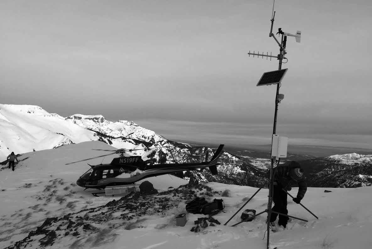
Observation sites should be selected so that measurements made at the site will be representative of the forecast area. The site should be as close as possible to avalanche starting zones and still permit regular observations. Exposure issues usually dictate separate sites for wind and precipitation measurements. When separate sites are deemed necessary, air temperature measure ments should be collected from both sites.
A meteorological study site will ideally be located in a level, open area that is devoid of large vegetation. The World Meteorological Organization (WMO) recommends a site 10 meters by 7 meters (WMO, 1996). This recommendation should be treated as an ideal, as significantly smaller sites may be more appropriate for observations in exposed mountain areas. The surface should
71
FIGURE D.1 A remote weather station. ! Colorado Avalanche Information Center
be cleared so that the ground cover consists of short grass or the predominate ground cover in the area. Instruments should be placed in a measurement site (approximately two-meter by two-meter area) at the center of the opening. A visual barrier or signs should surround the area to prevent unwary travelers from disturbing the study site.
Snowpack observation sites can be co-located with meteoro logical sites if adequate space is available. Snowpack and precip itation measurement sites should be sheltered from the wind. Sites that minimize snow drifting should be selected if wind effects cannot be avoided. The main requirement for wind sta tions is a good correlation between measurements at observation locations and avalanche starting zones.
D.3 INSTRUMENT EXPOSURE
Precipitation
For sites where precipitation measurements are made, it is rec ommended that the instrument (snow board, rain gauge, snow depth sensor, etc.) be at least as far from the nearest obsta cle (building, tree, fence post, etc.) as that obstacle is high. Precipitation sites should be devoid of sloping terrain if possible and away from depressions or hollows. Rooftop sites should be avoided. When practical or environmental constraints require deviating from these guidelines, the changes can be recorded in the metadata file (see Appendix C).
Precipitation gauges located at windy sites can seriously underestimate the actual precipitation amount. Gauge catch can be improved by the following methods listed in the order of effectiveness (WMO, 1996):
1. The vegetation height of the site can be maintained at the same height as the gauge orifice, thus maintaining a hori zontal wind flow over the gauge.
2. The effect listed in point 1 can be simulated by an artificial structure (i.e. fence).
3. The use of a wind shield such as an Alter or Nipher shield, or a similar device around the gauge orifice.
Many avalanche operations use ultrasonic distance instru ments to remotely monitor snow height. These gauges can be used to record both total snow height (HN) or interval values (e.g. HN24). The response of these instruments is affected by both air temperature (which can be addressed in the datalogger program) and the concentration of airborne particles.
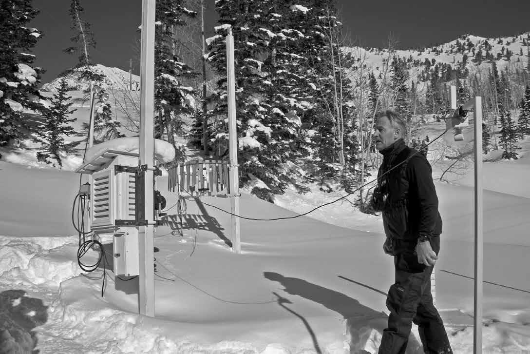
Temperature
Temperature instruments must be properly ventilated and sheltered from radiation sources. This can be accomplished by housing the instrument in a commercial radiation shield or instrument shelter. Manual and automated instruments can be co-located in a Stevenson screen. The screen door should open to the north to prevent solar heating of the temperature sensors.
72 APPENDIX D: OBSERVATION SITES FOR METEOROLOGICAL MEASUREMENTS
FIGURE D.2 The Utah Department of Transportation’s study site in Alta, Utah. ! Bruce Tremper
Temperature instruments should be located 1.25 m to 2 m above the surface (WMO, 1996). Ideally the instrument shel ter is mounted on an adjustable post so that a constant distance above the surface can be maintained. The instrument should be exposed to wind and sun (although properly shielded).
Depressions or hollows that can trap cold air should be avoided. Temperature measurements should not be made near buildings or on rooftops.
Relative Humidity
Instrument exposure issues for relative humidity measurements will depend on the measurement method. Relative humidity measurements in below freezing environments can be difficult and instrument selection is critical (and beyond the scope of these Guidelines). In general, instruments should be sheltered from direct solar radiation, atmospheric contaminants, precip itation and wind (WMO, 1996). Materials such as wood and some synthetic products can absorb and desorb water according to atmospheric humidity (WMO, 1996). If the enclosure is made of wood it should be coated in white enamel paint (creating a vapor barrier). Relative humidity instruments can be co-located with temperature instruments provided that these issues are addressed.
Wind
Anemometers should ideally be located atop a vibration-free, 10-meter (~30 ft) tower. Wind measurements can be dramati cally affected by the presence of upstream obstacles. Ideally, there should be no obstructions within a 100 m (~ 300 ft) radius of the anemometer (WMO, 1996). In mountainous terrain, where large obstacles are prevalent, anemometers at two or more locations can be used to gain adequate wind information in a variety of conditions. Local obstructions, such as the tower or other instru ments, should be a distance away from the wind sensor that is four to five times the diameter of the obstruction. These effects can be addressed by placing the wind sensor at the top of the tower.
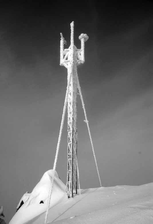
Several wind stations may be needed to obtain a reasonable estimate of wind effects within a forecast area. Considerable sep aration (vertical and horizontal) may be required to achieve a suitable representation of the actual wind field. It is essential that cup anemometers be horizontal to the underlying surface. All stations must be accessible in the winter either by foot, snow mobile or helicopter for occasional maintenance of equipment. Rime ice accretion is a common problem (Figure D.4) that can be addressed with heated sensors.
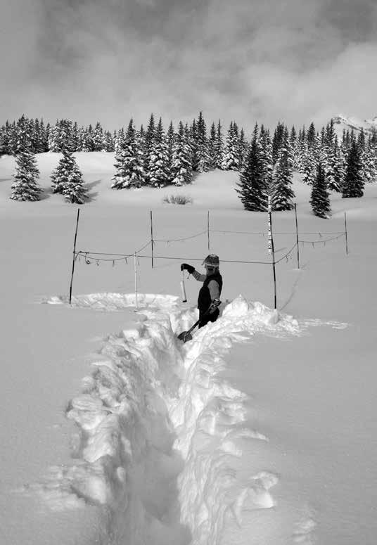
APPENDIX D: OBSERVATION SITES FOR METEOROLOGICAL MEASUREMENTS 73
FIGURE D.3 Snow study plot for manual observations. ! Ann Mellick
FIGURE D.4 A weather station coated in rime ice. ! John Stimberis
Radiation
Radiation processes have a large effect on snowpack stability and avalanche release. Instrument exposure issues will depend on the type of radiation measured and the direction of the radi ation (incoming or outgoing), but radiation can be measured at any study site. If only one radiation component can be mea sured, incoming shortwave radiation may be the most useful. However, both short and longwave components can benefit avalanche applications.

Incoming shortwave radiation can be measured in a flat open area. Sensors should be installed so that they are level and in locations that are not in the shadow of buildings, trees, and when possible, mountains (Figure D.4). Shadowing should be evaluated throughout the day and season for instrument placement. The effects of the tower will be minimized if the instrument is placed a significant distance from (long arm) and on the south side (in the Northern Hemisphere) of the tower. It may also be beneficial to place incoming shortwave sensors above the vegetation canopy.

74 APPENDIX D: OBSERVATION SITES FOR METEOROLOGICAL MEASUREMENTS
FIGURE D.5 Left: A remote weather station to monitor general atmospheric conditions. ! Kelly Elder Right: A study site to record manual and remote weather observations. ! Ethan Greene
APPENDIX E: AUTOMATED WEATHER STATIONS
E.1 INTRODUCTION
Automated measurements of snow and weather phenomena are extremely useful components of an observational record (World Meteorological Organization No. 8, 2018). Automated sites pro vide an uninterrupted record and yield information about areas that are not commonly visited. Automated measurements allow observers to fill in the periods between manual observations, and may provide key information that would otherwise be missed. In many cases it may be more practical to maintain a weather record that is a combination of manual and automated measure ments. When possible, automated measurements should be used to augment and not replace manual observations.
E.2 OBJECTIVES
The purpose of this Appendix is to:
• Establish common methods for recording and reporting data collected by automated stations
• Encourage uniformity of measurements
• Provide methods for combining manual and automated data
• Encourage methods that produce data that is compatible with other long-term records
E.3 COMBINING MANUAL AND AUTOMAT ED DATA
Maintaining a separate manual and automated data record is generally preferred. Replacing manual observations with auto mated measurements should only be employed when the oper ation headquarters are a significant distance from the avalanche terrain, or if access to a study site is unreliable.
Daily weather summaries that include a combination of man ual observations and automated measurements are often useful for operations that make decisions based on these data. This prac tice is not a problem until the data set is transmitted to another user or central database. Manual and automated records can be co-located as long as a careful record of the source and type of measurement is present in the metadata file (see Appendix C). However, maintaining separate manual and automated data records is recommended.
The most common parameters obtained from automated weather stations are wind speed, wind direction, and tempera ture. Automated measurements of precipitation and total snow depth have become more common with improvements in sensors. Automated depth sensors can be used to record valu able interval measurements at stations that can not be visited regularly.
Values for wind speed and direction for daily observation sheets can be obtained by recording the hourly average from the period during which the manual observations were made. Maximum and minimum temperatures can also be obtained from an automated station provided that system explicitly records these values. The 24-hour maximum and minimum temperature should be averages of a period no longer than one minute (WMO, 1996).
E.4 SAMPLING RATES AND AVERAGING PERIODS
The time interval between measurements (sampling rate) is an important and complex issue. Avalanche forecasting operations typically use a sampling rate of 3 to 5 seconds for temperature, wind, relative humidity, and pressure measurements. However, longer execution intervals (up to 60 sec) may be necessary at remote stations where power is limited. Precipitation measure ment rates will depend on the instrument. Snow depth sensors can be sampled at the same rate that data is stored (i.e. 10 min ute, 1 hour, etc.). Other precipitation sensors may require the computation of a running total rather than an average. These are practical solutions that work for many applications. Operations that require more robust sampling schemes are referred to World Meteorological Organization Publication No. 8 (see Appendix A for full reference).
Power constraints may dictate sampling schemes in remote locations. If these issues prevent continuous sampling, measure ments can be sampled for 5 minutes before the hour and data can be recorded and reported on the hour.
The period over which a parameter is averaged depends upon the application. Many avalanche forecasting operations find it useful to look at averages of 5- 10- or 15-minute periods. These short interval averages will be most useful during storm periods, while one-hour averages are more useful for daily operations. Parameters stored in six-hour averages will conform to other long-term records such as climatic datasets. It is recommended that one-hour averages be stored as the long-term record.
Most parameters measured at automated weather stations can be averaged with a simple arithmetic scheme. Wind direction is the most notable exception. Wind direction averages must be computed with a scheme that accounts for the circular nature of the values. Most data logger programming structures have a spe cific averaging scheme for these data. Otherwise it is common practice to use a vector representation of wind and average its two horizontal components (Fisher, 1993: p. 31).
75
APPENDIX F: ICSI CLASSIFICATION FOR SEASONAL SNOW ON THE GROUND
This Appendix reproduces the Grain Shape Classification (Appendix A) of the International Classification for Seasonal Snow on the Ground (Fierz and others, 2009). The full document can be downloaded at https://cryosphericsciences.org/publications/snowclassification/. The identification notes provided at the end of this Appendix (Rounded Polycrystals, Wind Crusts, Melt-freeze Crusts, Surface Hoar) are intended to supplement the Classification System.
TABLE F.1 Main and subclasses of grain shapes
MORPHOLOGICAL CLASSIFICATION
BASIC CLASSIFICATION
PRECIPITATION
ADDITIONAL INFORMATION ON PHYSICAL PROCESS AND STRENGTH
SUBCLASS SHAPE CODE PLACE OF FORMATION PHYSICAL
PROCESS
DEPENDENCE ON MOST IMPORTANT PARAMETERS
COMMON EFFECT ON STRENGTH
PARTICLES PP +
Columns ▭
Prismatic crystal, solid or hollow
Needles Needle-like, approximately cylindrical
PPco Cloud; temperature inversion layer (clear sky)
PPnd Cloud
Plates Plate-like, mostly hexagonal PPpl Cloud; temperature inversion layer (clear sky)
Stellars, Dendrites m
Irregular crystals n
Six-fold star-like, planar or spatial PPsd Cloud; temperature inversion layer (clear sky)
Growth from water vapor at –3 to –8 °C and below–30 °C
Growth from water vapor at high supersaturation at –3 to –5 ° C and below –60 °C
Growth from water vapor at 0 to –3 °C and –8 to –70 °C
Growth from water vapour at high supersaturation at 0 to –3 ° C and at –12 to –16 °C
Clusters of very small crystals PPir Cloud Polycrystals growing in varying environmental conditions
Graupel o Heavily rimed particles, spherical, conical, hexagonal, or irregular in shape
Hail � Laminar internal structure, translucent or milky glazed surface
Ice Pellets ◬
Rime
Transparent, mostly small spheroids
PPgp Cloud
Heavy riming of particles by accretion of supercooled water droplets Size: ≤ 5 mm
PPhl Cloud
Growth by accretion of supercooled water Size: > 5 mm
PPip Cloud
Freezing of raindrops or refreezing of largely melted snow crystals or snowflakes (sleet) Graupel or snow pellets encased in thin ice layer (small hail) Size: both ≤ 5 mm
Irregular deposits or longer cones and needles pointing into the wind
PPrm Onto surface as well as on freely exposed objects
Accretion of small, supercooled fog droplets frozen in place. Thin breakable crust forms on snow surface if process continues long enough
Increase with fog density and exposure to wind
76
See Notes on next page
MORPHOLOGICAL CLASSIFICATION
ADDITIONAL INFORMATION ON PHYSICAL PROCESS AND STRENGTH
BASIC CLASSIFICATION SUBCLASS SHAPE CODE PLACE OF FORMATION PHYSICAL PROCESS
MACHINE MADE SNOW
MM b
Round polycrys talline particles b
Small spherical particles, often showing protrusions, a result of the freezing process, may be partially hollow
MMrp Atmosphere, near surface
Machined snow, i.e., freezing of very small water droplets from the surface inward
DEPENDENCE ON MOST IMPORTANT PARAMETERS
Liquid water content depends mainly on air temperature and humidity but also on snow density and grain size
COMMON EFFECT ON STRENGTH
In dry conditions, quick sintering results in rapid strength increase
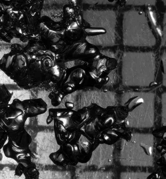
Crushed ice particles t
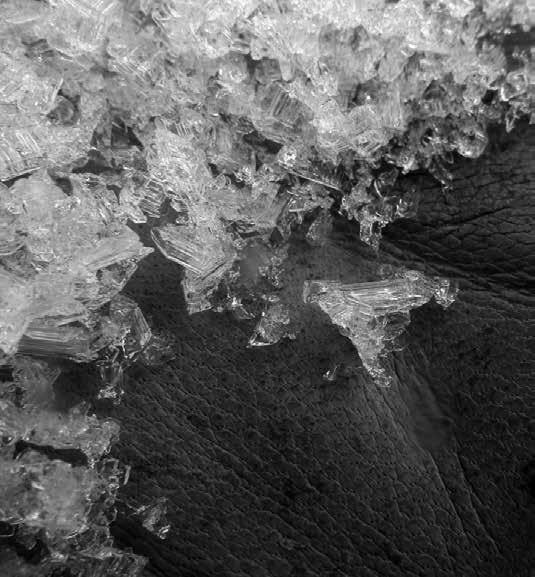
References: Fauve et al., 2002
Ice plates, shard-like
MMci Ice generators
Machined ice, i.e., production of flake ice, subsequent crushing, and pneu matic distribution
All weather safe
Precipitation Particles Notes: A subscript “r” modifier is used to denote rimed grains in the Decomposing and Fragmented Particles (DF) major class and the Precipitation Particles (PP) major class and its subclasses except for gp, hl, ip, rm (Example: PP-r). Hard rime is more compact and amorphous than soft rime and may build out as glazed cones or ice feathers (AMS, 2000). The above subclasses do not cover all types of particles and crystals one may observe in the atmosphere. See the references below for a more comprehensive coverage. References: Magono & Lee, 1966; Bailey & Hallett, 2004; Dovgaluk & Pershina. 2005; Libbrecht, 2005
APPENDIX F: ICSI CLASSIFICATION FOR SEASONAL SNOW ON THE GROUND 77
FIGURE F.1 Left: Poly crystals (MFpc) in the Melt Forms class. ! Ethan Greene Right: Large heavily striated crystals (DHla) in the Depth Hoar class. ! Jeff Davis
MORPHOLOGICAL CLASSIFICATION
BASIC CLASSIFICATION SUBCLASS SHAPE
CODE
ADDITIONAL INFORMATION ON PHYSICAL PROCESS AND STRENGTH
PLACE OF FORMATION PHYSICAL PROCESS
DEPENDENCE ON MOST IMPORTANT PARAMETERS
DECOMPOSING AND FRAGMENTED PRECIPITATION PARTICLES
Partly de composed precip itation particles c
Characteristic shapes of precipi tation particles still recognizable; often partly rounded
DF
DFdc Within the snowpack; re cently depos ited snow near the surface, usually dry
Decrease of surface area to reduce sur face free energy; also fragmentation due to light winds lead to initial break up
Speed of de composition decreases with decreas ing snow tem peratures and decreasing temperature gradients
COMMON EFFECT ON STRENGTH
Regains cohesion by sintering after initial strength de creased due to decom position process
cWind-bro ken pre cipitation particles v
Shards or fragments of precipitation particles

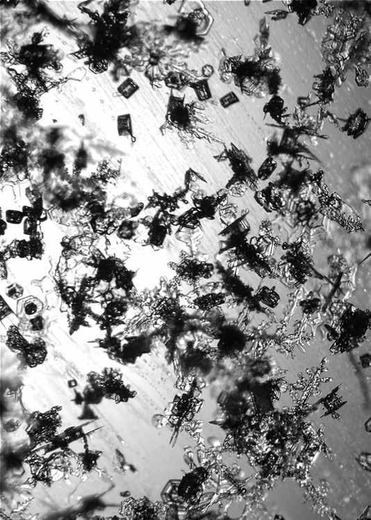
DFbk Surface layer, mostly recent ly deposited snow
Saltation particles are fragmented and packed by wind, of ten closely; fragmen tation often followed by rounding
Fragmen tation and packing increase with wind speed
Quick sintering re sults in rap id strength increase
78 APPENDIX F: ICSI CLASSIFICATION FOR SEASONAL SNOW ON THE GROUND
FIGURE F.2 Left: New snow that contains an array of precipitation particles including columns (PPco), plates (PPpl), and stellar crystals (PPsd)
Right: Rounded snow grains (RR). ! Kelly Elder
MORPHOLOGICAL CLASSIFICATION
ADDITIONAL INFORMATION ON PHYSICAL PROCESS AND STRENGTH
BASIC CLASSIFICATION SUBCLASS SHAPE CODE PLACE OF FORMATION PHYSICAL PROCESS
ROUNDED GRAINS
Small rounded particles w
●
DEPENDENCE ON MOST IMPORTANT PARAMETERS
Rounded, usually elongated particles of size <0.25 mm; highly sintered
RG
RGsr Within the snowpack, dry snow
Decrease of specific surface area by slow decrease of number of grains and increase of mean grain diame ter. Small equilibrium growth form
Growth rate increases with increasing tempera ture; growth slower in high density snow with smaller pores
COMMON EFFECT ON STRENGTH
Strength due to sin tering of the snow grains [1]. Strength increases with time, settle ment and decreasing grain size
Large rounded particles ●
Rounded, usually elongated particles of size > o.25 mm; well sintered
RGlr Within the snowpack, dry snow
Grain-to-grain vapor diffusion due to low temperature gra dients, i.e., mean excess vapor density remains below critical value for kinetic growth. Large equi librium growth form
Same as above Same as above
Wind packed y
Small, broken or abraded, closely packed particles; well sintered
RGwp Surface layer, dry snow
Packing and frag mentation of wind transported snow particles that round off by interaction with each other in the sal tation layer. Evolves into either a hard but usually breakable wind crust or a thicker wind slab
Hardness increases with wind speed, decreasing particle size and moderate temperature
High number of contact points and small size causes rap id strength increase through sintering
Faceted rounded particles
Faceted crystals with rounding facets and corners
RGxf Within the snowpack, dry snow
Growth regime changes if mean excess vapor density is larger than criti cal value for kinetic growth. Accordingly, this transitional form develops facets as temperature gradient increases
Grains are changing in response to an increasing temperature gradient
Reduction in num ber of bonds may decrease strength
Round Grains Notes: Both wind crusts and wind slabs are layers of small, broken or abraded, closely packed and well-sintered particles. The former are thin irregular layers whereas the latter are thicker, often dense layers, usually found on lee slopes. Both types of layers can be represented either as sub-class RGwp or as RGsr along with proper grain size, hardness and/or density. If the grains are smaller than about 1 mm, an observer will need to consider the process at work to differentiate RGxf from FCxr. References: [1] Colbeck, 1997
APPENDIX F: ICSI CLASSIFICATION FOR SEASONAL SNOW ON THE GROUND 79
MORPHOLOGICAL CLASSIFICATION
BASIC CLASSIFICATION SUBCLASS SHAPE
FACETED CRYSTALS
CODE
ADDITIONAL INFORMATION ON PHYSICAL PROCESS AND STRENGTH
PLACE OF FORMATION PHYSICAL PROCESS
DEPENDENCE ON MOST IMPORTANT PARAMETERS
COMMON EFFECT ON STRENGTH
Solid faceted particles e
Solid faceted crys tals; usually hexago nal prisms
FC e
FCso Within the snowpack; dry snow
Grain-to-grain vapour diffusion driven by large enough tem perature gradient, i.e., excess vapour density is above crit ical value for kinetic growth
Solid kinetic growth form, i.e., a solid crys tal with sharp edges and corners as well as glassy, smooth faces
Growth rate increases with temperature, increasing temperature gradient, and decreasing density; may not grow to larger grains in high density snow because of small pores
Strength decreas es with increasing growth rate and grain size
Near surface faceted particles
Faceted crystals in surface layer
FCsf Within the snowpack but right beneath the surface; dry snow
May develop directly from Precipitation Particles (PP) or Decomposing and Fragmented particles (DFdc) due to large, near-surface tem perature gradients [1] Solid kinetic growth form (see FCso above) at early stage
Temperature gradient may periodically change sign but remains at a high ab solute value
Lowstrength snow
Rounding faceted particles
Rounded, usually elongated particles with developing facets
FCxr Within the snowpack, dry snow
Trend to a transition al form reducing its specific surface area; corners and edges of the crystals are rounding off
Grains are rounding off in response to a decreasing temperature gradient
Faceted Crystals Notes: Once buried, FCsf are hard to distinguish from FCso unless the observer is familiar with the evolution of the snowpack.
FCxr can usually be clearly identified for crystals larger than about 1 mm. In case of smaller grains, however, an observer will need to consider the process at work to differentiate FCxr from RGxf. References: [1] Birkeland, 1998
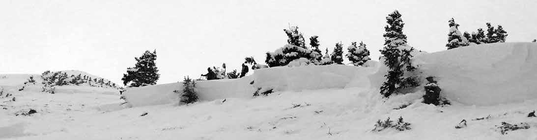
80 APPENDIX F: ICSI CLASSIFICATION FOR SEASONAL
THE
SNOW ON
GROUND
FIGURE F.3 Crown face of a fresh slab avalanche that released on basal facets. ! Doug Krause
MORPHOLOGICAL CLASSIFICATION
ADDITIONAL INFORMATION ON PHYSICAL PROCESS AND STRENGTH
BASIC CLASSIFICATION SUBCLASS SHAPE CODE PLACE OF FORMATION PHYSICAL PROCESS
DEPTH HOAR DH
Hollow cups ^
Striated, hollow skeleton type crystals; usually cup-shaped
^
Hollow prisms E
Chains of depth hoar
Prismatic, hollow skeleton type crystals with glassy faces but few striations
DHcp Within the snowpack, dry snow
Grain-to-grain vapour diffusion driven by large temperature gradient, i.e., excess vapour den sity is well above critical value for kinetic growth. Formation of hollow or partly solid cup-shaped kinetic growth crystals [1]
DEPENDENCE ON MOST IMPORTANT PARAMETERS
COMMON EFFECT ON STRENGTH
See FCso. Usually fragile but strength in creases with density
Large striated crystals
Hollow skeleton type crystals ar ranged in chains
DHpr Within the snowpack, dry snow
DHch Within the snowpack, dry snow
Snow has completely recrystallized; high temperature gradient in low density snow, most often prolonged [2]
Snow has completely recrystallized; inter granular arrangement in chains; most of the lateral bonds between columns have disap peared during crystal growth
High recrys tallization rate for long period and low density snow facilitates formation
High recrys tallization rate for long period and low density snow facilitates formation
May be very poorly bonded
Very fragile snow
Round ing depth hoar
Large, heavily striated crystals; either solid or skeleton type
DHla Within the snowpack, dry snow
Evolves from earli er stages described above; some bonding occurs as new crystals are initiated [2]
Longer time required than for any other snow crystal; long periods of large tempera ture gradient in low densi ty snow are needed
Regains strength
Hollow skeleton type crystals with rounding of sharp edges, corners, and striations
DHxr Within the snowpack, dry snow
Trend to a form reduc ing its specific surface area; corners and edges of the crystals are rounding off; faces may lose their relief, i.e., striations and steps disappear slowly. This process affects all sub classes of depth hoar
Grains are rounding off in response to a decreasing temperature gradient
May regain strength
Depth Hoar Notes: DH and FC crystals may also grow in snow with density larger than about 300 kg m3 such as found in polar snow packs or wind slabs. These may then be termed ‘hard’ or ‘indurated’ depth hoar [3]. References: [1] Akitaya, 1974; Marbouty, 1980; Fukuzawa & Akitaya, 1993; Baunach et al., 2001; Sokratov, 2001; [2] Sturm & Benson, 1997; [3] Akitaya, 1974; Benson & Sturm, 1993
APPENDIX F: ICSI CLASSIFICATION FOR SEASONAL SNOW ON THE GROUND 81
MORPHOLOGICAL CLASSIFICATION ADDITIONAL INFORMATION ON PHYSICAL PROCESS AND STRENGTH
OF FORMATION
PHYSICAL PROCESS
SURFACE HOAR SH
Surface hoar crystals ∨
Striated, usually flat crystals; some times nee dle-like
SHsu Usually on cold snow surface relative to air temperature; sometimes on freely exposed objects above the surface (see notes)
∨
DEPENDENCE ON MOST IMPORTANT PARAMETERS
Rapid kinetic growth of crystals at the snow surface by rapid transfer of water vapour from the atmosphere toward the snow surface; snow surface cooled to below ambient temperature by radiative cooling
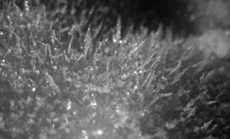
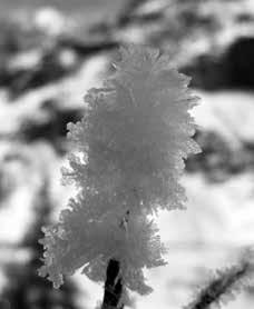
Both increased cooling of the snow surface below air tem perature as well as increasing relative humidity of the air cause growth rate to increase. In high water vapour gradient fields, e.g., near creeks, large feathery crystals may develop
COMMON EFFECT ON STRENGTH
Fragile, extremely low shear strength; strength may remain low for extended periods when bur ied in cold dry snow
Cav ity or crevasse hoar J
Striated, planar or hollow skeleton type crys tals grown in cavities; orienta tion often random
SHcv Cavity hoar is found in large voids in the snow, e.g., in the vicinity of tree trunks, buried bushes [1] Cre vasse hoar is found in any large cooled space such as cre vasses, cold storage rooms, boreholes, etc.
Kinetic growth of crystals forming anywhere where a cavity, i.e., a large cooled space, is formed or present in which water vapour can be deposited under calm, still condi tions [2]
Round ing surface hoar K
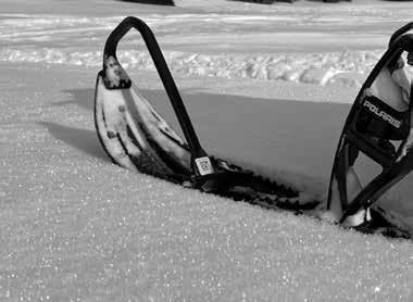
Surface hoar crys tal with rounding of sharp edges, corners and stria tions
SHxr Within the snowpack; dry snow Trend to a form reducing its specific surface area; corners and edges of the crystals are rounding off; faces may loose their relief, i.e., striations and steps disappear slowly
Grains are rounding off in response to a decreasing tem perature gradient
May regain strength
Surface Hoar Notes: It may be of interest to note more precisely the shape of hoar crystals, namely plates, cups, scrolls, needles and col umns, dendrites, or composite forms [3]. Multi-day growth may also be specified. Surface hoar may form by advection of nearly saturated air on both freely exposed objects and the snow surface at subfreezing temperatures. This type of hoarfrost deposit makes up a substantial part of accumulation in the inland of Antarctica. It has been termed 'air hoar’ (see [2] and AMS, 2000). Crevasse hoar crystals are very similar to depth hoar. References: [1] Akitaya, 1974; [2] Seligman, 1936; [3] Jamieson & Schweizer, 2000
82 APPENDIX F: ICSI CLASSIFICATION FOR SEASONAL SNOW ON THE GROUND
BASIC CLASSIFICATION SUBCLASS SHAPE CODE PLACE
FIGURE F.4 Surface hoar formations. ! Doug Krause and Mark Staples
MORPHOLOGICAL CLASSIFICATION
ADDITIONAL INFORMATION ON PHYSICAL PROCESS AND STRENGTH
BASIC CLASSIFICATION SUBCLASS SHAPE CODE PLACE OF FORMATION PHYSICAL PROCESS
DEPENDENCE ON MOST IMPORTANT PARAMETERS
COMMON EFFECT ON STRENGTH
MF h
MELT FORMS
Clustered rounded grains
Clustered rounded crystals held by large ice-to-ice bonds; water in internal veins among three crystals or two grain boundaries
MFcl At the surface or within the snowpack; wet snow
Rounded polycrys tals M
Individual crystals are frozen into a solid polycrystalline particle, either wet or refrozen
MFpc At the surface or within the snowpack
Wet snow at low water content (pendular regime), i.e., holding free liquid water; clusters form to minimize surface free energy
Melt-freeze cycles form polycrystals when water in veins freezes; either wet at low water content (pendular regime) or refrozen
Meltwater can drain; too much water leads to MFsl; first freezing leads to MFpc
Particle size increases with number of melt-freeze cycles; radi ation pene tration may restore MFcl; excess water leads to MFsl
Ice-to-ice bonds give strength
High strength in the frozen state; lower strength in the wet state; strength in creases with number of melt-freeze cycles
Slush N Separated rounded particles completely immersed in water
MFsl Water saturated, soaked snow; found within the snowpack, on land or ice surfaces, but also as a viscous floating mass in water after heavy snowfall.
Wet snow at high liquid water content (funicular regime); poorly bonded, fully rounded single crys tals–and polycrystals–form as ice and water are in thermodynamic equilibrium
Water drain age blocked by capillary barrier, imperme able layer or ground; high energy input to the snowpack by solar radia tion, high air temperature or water input (rain)
Little strength due to decaying bonds
Meltfreeze crust
Oh
Crust of recogniz able melt-freeze polycrystals
MFcr At the surface Crust of melt-freeze polycrystals from a surface layer of wet snow that refroze after having been wetted by melt or rainfall; found either wet or refrozen
Particle size and density increases with number of melt-freeze cycles
Strength in creases with number of melt-freeze cycles
Melt Form Notes: Melt-freeze crusts MFcr form at the surface as layers at most a few centimeters thick, usually on top of a subfreezing snowpack. Rounded polycrystals MFpc will rather form within the snowpack. MFcr usually contain more refrozen water than MFpc and will not return to MFcl. Both MFcr and MFpc may contain a recognizable minority of other shapes, particularly large kinetic growth form FC and DH. See the guidelines (Appendix C) for examples on the use of the MFcr symbol.
APPENDIX F: ICSI CLASSIFICATION FOR SEASONAL SNOW ON THE GROUND 83
MORPHOLOGICAL CLASSIFICATION ADDITIONAL INFORMATION ON PHYSICAL PROCESS AND STRENGTH
BASIC CLASSIFICATION SUBCLASS SHAPE CODE PLACE OF FORMATION PHYSICAL PROCESS
IF
Ice layer i Horizontal ice layer
▅
Ice col umn
Vertical ice body
IFil Within snow pack Rain or meltwater from the surface percolates into cold snow where it refreezes along layer-par allel capillary barriers by heat conduction into surrounding subfreezing snow, i.e., snow at T < 0 °C; ice layers usually retain some degree of permeability
IFic Within snow pack layers
Basal ice Basal ice layer
Rain crust Thin, trans parent glaze or clear film of ice on the surface
Sun crust, Firnspie gel
Thin, trans parent and shiny glaze or clear film of ice on the surface
Draining water within flow fingers freezes by heat conduction into surround ing subfreezing snow, i.e., snow at T < 0 °C
IFbi Base of snow pack Melt water ponds above substrate and freezes by heat conduction into cold substrate
IFrc At the surface Results from freezing rain on snow; forms a thin surface glaze
IFsc At the surface Melt water from a surface snow layer refreezes at the surface due to radia tive cooling; decreasing shortwave absorption in the forming glaze en hances greenhouse effect in the underlying snow; additional water vapour may condense below the glaze [1]
DEPENDENCE ON MOST IMPORTANT PARAMETERS
COMMON EFFECT ON STRENGTH ICE FORMATIONS
Depends on tim ing of percolating water and cycles of melting and refreezing; more likely to occur if a stratification of fine over coarsegrained layers exists
Ice layers are strong but strength decays once snow is complete ly wetted
Flow fingers more likely to occur if snow is highly stratified; freezing enhanced if snow is very cold
Formation enhanced if substrate is im permeable and very cold, e.g., permafrost
Droplets have to be supercooled but coalesce be fore freezing
Builds during clear weather, air temperatures below freezing and strong solar radiation; not to be confused with melt -freeze crust MFcr
Weak slush layer may form on top
Thin break able crust
Thin break able crust
Ice Formation Notes: In ice formations, pores usually do not connect and no individual grains or particles are recognizable, contrary to highly porous snow. Nevertheless, some permeability remains, in particular when wetted, but to much a lesser degree than for porous melt forms. Most often, rain and solar radiation cause the formation of melt-freeze crusts MFcr. Discontinuous ice bodies such as ice lenses or refrozen flow fingers can be identified by appropriate remarks. References: [1] Ozeki & Akitaya, 1998
84 APPENDIX F: ICSI CLASSIFICATION FOR SEASONAL SNOW ON THE GROUND
ROUNDED POLYCRYSTALS, WIND CRUSTS, AND MELT-FREEZE CRUSTS
To distinguish between rounded polycrystals (MFpc) and a melt-freeze crust (MFcr), consider the structural units. If a crust layer is broken apart, the result is lumps of variable size since the crust (of indeterminate length and width) is the structural unit. If a portion of a layer of frozen rounded polycrystals is broken apart, the result is quite consistently sized particles (the individual polycrystals).
When formed by freezing rain, rain crusts (IRrc) are often thin, fragile transparent layers that form on the surface. Rain more commonly forms melt-freeze crust (MFcr), which can vary from thin (several mm to 1 cm) to thick (>5 cm) layers.
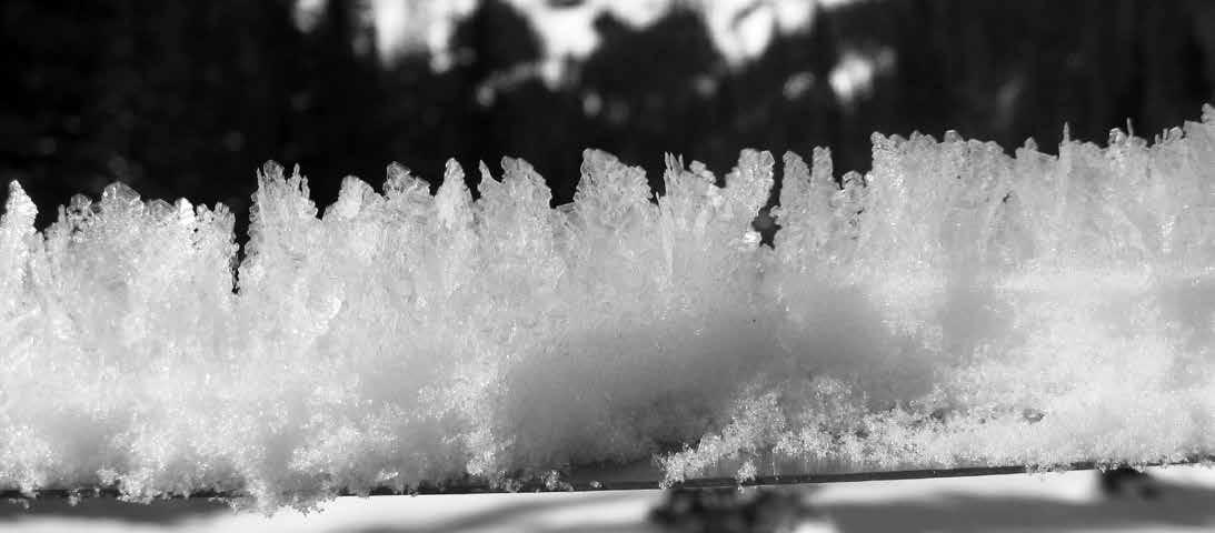
Sun crusts (IFsc) are thin, fragile transparent layers that form on the surface. More commonly, direct sun causes a melting of the snow that results in a melt-freeze crust (MFcr).
Wind crusts (RGwp) are thin irregular layers of small, broken or abraded, closely packed and well-sintered particles (usually found on windward slopes). The particles in these layers may be similar in appearance to those in wind slabs (usually found on lee slopes); however, some authors report that particle size is more variable in wind crusts than wind slabs.
SURFACE HOAR
Sub-classes listed in Table F.2 can be used to record different types of surface hoar (SH).
TABLE F.2 Sub-classes of surface hoar (based on Jamieson and Schweizer, 2000)
SUBCLASS DESCRIPTION
i. Needle
ii. Plate
iii. Dendrite
iv. Cup or scrolls
FORMATION TEMPERATURE
Primarily one-dimensional, sometimes spike- or sheath-like Below -21°C
Two-dimensional sector plate; usually wedge shaped and narrow at base. Usually striated when formed; however, the striations may disap pear while buried -10°C to -21°C
Two-dimensional form with numerous branches; often feather-like in appearance; narrow at base -10°C to -21°C
Three-dimensional; these form with narrow base on surface of the snowpack; once separated from the snowpack, these forms can be indistinguishable from depth hoar-cup crystals
v. Composite forms Combinations of shapes associated with subclasses i to iv
Refer to Fierz and others (2009) for further explanation of shapes, place of formation, classifications, physical processes and common effects on strength. The document is online at: https://cryosphericsciences.org/publications/snow-classification/.
APPENDIX F: ICSI CLASSIFICATION FOR SEASONAL
THE GROUND 85
SNOW ON
FIGURE F.5 Large surface hoar formed in a valley bottom. ! Doug Krause
APPENDIX G: AVALANCHE DANGER, HAZARD, AND SNOW STABILITY SCALES
G.1 INTRODUCTION
There are many ways to communicate the current avalanche conditions. Categorical scales of avalanche danger, avalanche hazard, and snow stability can improve communication between forecasters and customers. Forecasting operation managers should select an appropriate scale based on the definitions that follow. The scales presented in this Appendix are examples of commonly used communication methods.
G. 2 DEFINITIONS
Stability — The chance that avalanches do not initiate. Stability is analyzed in space and time relative to a given triggering level or load.
Exposure — An element or resource (person, vehicle, structure, etc.) that is subject to the impact of a specific natural hazard. Hazard, Avalanche — The potential for an avalanche(s) to cause damage to something of value. It is a combination of the likeli hood of triggering and the destructive size of the avalanche(s). It implies the potential to affect people, facilities or things of value, but does not incorporate vulnerability or exposure to avalanches. Avalanche danger and hazard are often used inter changeably and are commonly expressed using relative terms such as high, moderate and low.
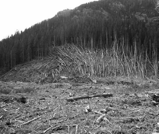
Risk — The chance of something happening that will have an impact on an element (person, vehicle, structure, etc.). A risk can often be specified in terms of an event or circumstance and the consequences that may follow. Risk is evaluated in terms of a combination of the consequences of an event and its likeli hood. See the Glossary (Appendix A) for a standard definition of Risk
Vulnerability — The degree to which an exposed element (per son, vehicle, structure, etc.) is susceptible the impact of a spe cific natural hazard.
G. 3 GENERAL GUIDELINES FOR THE USE OF AVALANCHE CONDITIONS SCALES
Avalanche conditions within a forecast area can be separated based on terrain or snowpack characteristics.
Specify the area based on:
1. Elevations
a. Numerical range
b. Geographic feature (i.e. Alpine, Treeline, Below Treeline)
2. Aspect
3. Slope angle
4. Specific conditions such as wind loaded slopes or depth of new snow
5. Spatial extent (localized or widespread)
6. Time of day
Timberline (treeline) describes a transition area between closed forest and the open treeless areas above.
Where practical give the expected stability trend for the next 12 to 24 hours. Use the terms: improving, steady, and decreasing stability to describe the trend.
Specify a confidence level in the ratings when appropriate; describe sources of uncertainty in forecast. Note the level of the unstable layer in the snowpack (i.e. near surface, mid level, deep). Observers may qualify the rating based on:
• Topography (aspect, slope angle, etc.)
• Spatial extent (localized or widespread)
• Time of day
G.4 SNOW STABILITY SCALE
Stability refers to the chance that avalanches will not initiate, and does not predict the size or potential consequences of expected ava lanches. Stability scales are sometimes used operationally in combi nation with variables such as slope aspect, elevation, and temporal effects. The Avalanche Danger Scale (Section G.5) is the preferred method for communicating avalanche conditions to the public. Statements about avalanche activity take precedence over results of stability tests. For regional and larger forecast areas, isolated natural avalanches may occur even when stability for the area as a whole is good.
Definitions / Examples
• Natural avalanches: Avalanches triggered by weather events such as snowfall, rain, wind, temperature changes, etc.
• Heavy load: A cornice fall, a compact group of people, a snowmobile or explosives.
• Light load: A single person, or a small cornice fall.
• Isolated terrain features: Extreme terrain; steep convex rolls; localized dispersed areas (pockets) without readily specifi able characteristics.
• Specific terrain features: Lee slopes, sun-exposed aspects.
• Certain snowpack characteristics: Shallow snowpack with faceted grains, persistent weaknesses, identified weaknesses.
86
FIGURE G.1 Vegetation damage from a large avalanche.
! John Stimberis
FIGURE G.2 Widespread avalanche activity within a single drainage. ! Craig Sterbenz
TABLE G.1 Snow Stability Rating System
STABILITY
STABILITY RATING
EXPECTED AVALANCHE ACTIVITY
COMMENT ON SNOW STABILITY NATURAL AVALANCHES (excluding avalanches triggered by icefall, cornice fall, or rock fall)
Very Good (VG) Snowpack is stable No natural avalanches expected
Good (G) Snowpack is mostly stable No natural avalanches expected
Fair (F)
Poor (P)
Very Poor (VP)
Snowpack stability var ies considerably with terrain, often resulting in locally unstable areas
Snowpack is mostly unstable
Isolated natural avalanches on specific terrain features
Natural avalanches in areas with specif ic terrain features or certain snowpack characteristics
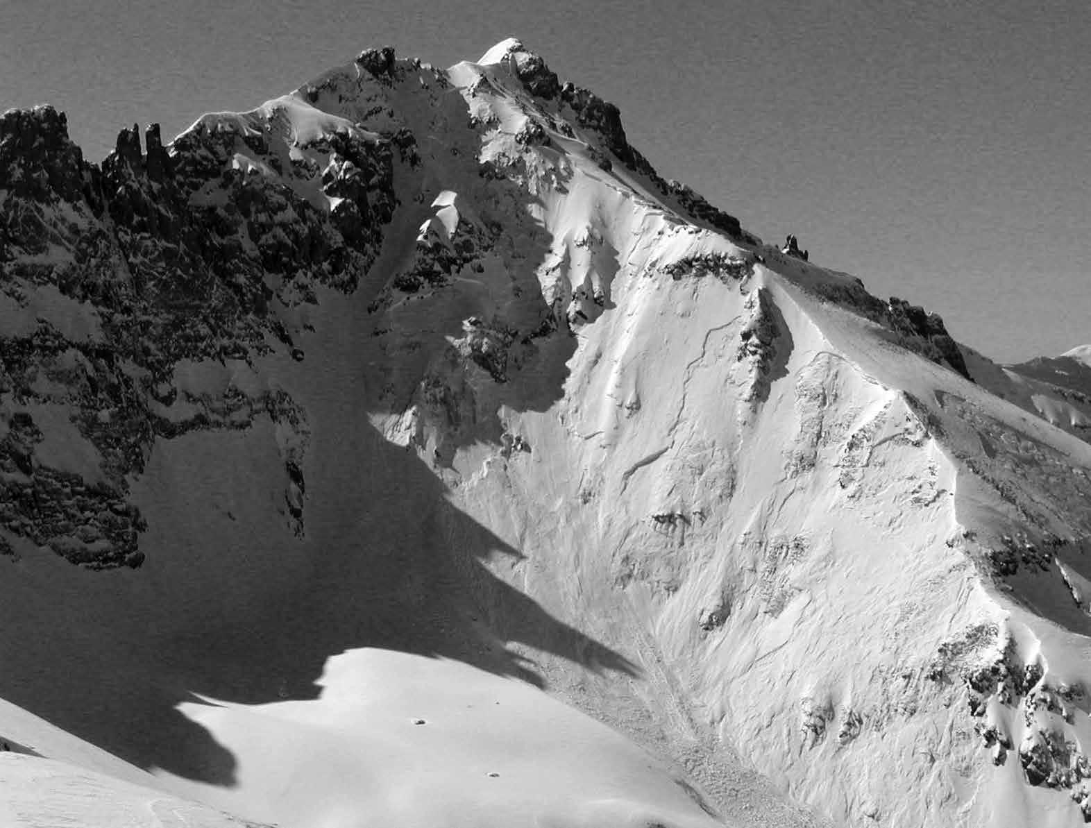
Snowpack is very unstable Widespread natural avalanches
TRIGGERED AVALANCHES (including avalanches triggered by human action, icefall, cornice fall, rock fall or wildlife)
Avalanches may be triggered by very heavy loads such as large cornice falls or loads in isolated terrain features
Avalanches may be triggered by heavy loads in isolated terrain features
Avalanches may be triggered by light loads in areas with specific terrain fea tures or certain snowpack characteristics
EXPECTED RESULTS OF STABILITY TESTS
Generally little or no result
Generally moderate to hard results
Generally easy to moderate results
Avalanches may be triggered by light loads in many areas with sufficiently steep slopes Generally easy results
Widespread triggering of avalanches by light loads Generally very easy to easy results
APPENDIX G: AVALANCHE DANGER, HAZARD, AND SNOW STABILITY SCALES 87
G.5 AVALANCHE DANGER SCALE
The Avalanche Danger Scale presented in this Appendix is used by regional avalanche forecast centers in the United States. The scale was designed to facilitate communication between forecasters and the public. The categories represent the probability of avalanche activity and recommend travel precautions.
Avalanche danger is determined by the likelihood, size, and distribution of avalanches.
Safe backcountry travel requires training and experience. You control your risk by choosing when, where, and how you travel.
North American Public Avalanche Danger Scale Danger Level Travel Advice
Likelihood
Extraordinarily dangerous avalanche conditions. Avoid all avalanche terrain.
4 - High
2 - Moderate
1 - Low
Very dangerous avalanche conditions. Travel in avalanche terrain not recommended.
Dangerous avalanche conditions. Careful snowpack evaluation, cautious route-finding, and conservative decision-making essential.
Heightened avalanche conditions on specific terrain features. Evaluate snow and terrain carefully; identify features of concern.
Generally safe avalanche conditions. Watch for unstable snow on isolated terrain features.
Natural and human-triggered avalanches certain.
Very large avalanches in many areas.5 - Extreme
Natural avalanches likely; human-triggered avalanches very likely.
Size and Distribution 3 - Considerable
Natural avalanches possible; human-triggered avalanches likely.
Large avalanches in many areas; or very large avalanches in specific areas.
Small avalanches in many areas; or large avalanches in specific areas; or very large avalanches in isolated areas.
Natural avalanches unlikely; human-triggered avalanches possible.
Natural and human-trigged avalanches unlikely.
FIGURE G.3 The North American Public Avalanche Danger Scale. (Statham et al., 2010)
Small avalanches in specific areas; or large avalanches in isolated areas.
Small avalanches in isolated areas or extreme terrain.
88 APPENDIX G: AVALANCHE DANGER,
AND SNOW STABILITY
HAZARD,
SCALES
TABLE G.2 Color Standards for the North American Public Avalanche Danger Scale DANGER LEVEL CMYK RGB WEB 5 Extreme (0, 64, 100, 100) (35, 31, 32) 231F20 4 High (0, 100, 100, 0) (237, 28, 36) ED1C24 3 Considerable (0, 50, 100, 0) (247, 148, 30) F7941E 2 Moderate (0, 0, 100, 0) (255, 242, 0) FFF200 1 Low (70, 0, 100, 0) (80, 184, 72) 50B848
G.6 AVALANCHE HAZARD SCALE
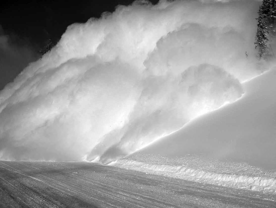
Avalanche hazard scales can be used when forecasting the threat of avalanches to structures and transpor tation arteries. The scale should be tailored for each individual operation. Figure G.5 contains a scale used by the Colorado Avalanche Information Center/ Colorado Department of Transportation. This scale is presented as an example of an operational avalanche hazard scale. Figure G.5 includes the entire scale, but columns can be included or excluded for different applications.
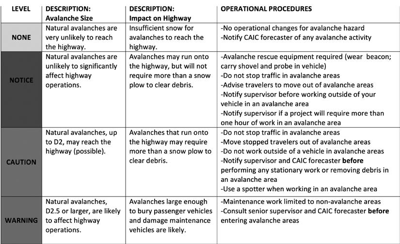
APPENDIX G: AVALANCHE DANGER, HAZARD, AND SNOW STABILITY SCALES 89
FIGURE G.4 An explosive triggered avalanche strikes US-160 near Wolf Creek Pass, Colorado. ! Mark Mueller
FIGURE G.5 An avalanche hazard rating scale used by the Colorado Avalanche Information Center and Colorado Department of Transportation. Provided as an example of a scale created for a specific application.
G.7 CONCEPTUAL MODEL OF AVALANCHE HAZARD
Statham et al. (2018) present a conceptual model of avalanche hazard that is widely used in avalanche safety applications throughout North America. The model is a tool that can be universally applied to all types of avalanche safety applications and directly inform risk mitigation decisions. The manuscript provides a complete overview of the model, how it was created, and how it can be applied. This section includes descriptions of several key elements of the model.
TABLE G.3 Spatial distribution (after Statham et al. 2018)
DISTRIBUTION SPATIAL DENSITY EVIDENCE
Isolated
The avalanche problem is spotty and found in only a few terrain features
Specific The avalanche problem exists in terrain fea tures with common characteristics
Widespread The avalanche problem is found in many loca tions and terrain features
is the evidence distributed?
Evidence is rare and hard to find
Evidence exists but is not always obvious
Evidence is everywhere and easy to find
hard is it to find?
FIGURE G.6 Likelihood of avalanche(s) results from the integration of spatial distribution and sensitivity to triggers (after Müller et al., 2016, and Statham el al., 2018).
90 MANUAL SNOW AND WEATHER OBSERVATIONS
Comment How
How
WIDESPREAD Unlikely Possible Very Likely Almost Certain SPECIFIC Unlikely Possible Likely Very Likely ISOLATED Unlikely Unlikely Possible Likely UNREACTIVE STUBBORN REACTIVE TOUCHY SPATIAL DISTRIBUTION SENSITIVITY TO TRIGGERS
TABLE
Types of avalanche problems (after Statham et al. 2018)
NAME DESCRIPTIONA FORMATION PERSISTENCE
Dry loose avalanche problem
Wet loose avalanche problem
Cohesionless dry snow starting from a point. Also called a sluff or point release
Cohesionless wet snow starting from a point. Also called a sluff or point release
Surface layers of new snow crystals that lack cohesion, or surface layers of faceted snow grains that lose cohesion
Snow becomes wet and cohesionless from melting or liquid precipitation
Generally lasts hours to days when associated with new snow, and longer when associated with facets
Persistence correlates with warm air temperatures, wet snow or rain, and/or solar radiation
Storm slab avalanche problem
Wind slab avalanche problem
Cohesive slab of soft new snow. Also called a direct-action avalanche
Cohesive slab of locally deep, wind-deposited snow
Cohesive slab of new snow creates short-term instability within the storm snow or at the old snow interface
Wind transport of falling snow or soft surface snow. Wind action breaks snow crystals into smaller particles and packs them into a cohesive slab overlying a nonpersistent weak layer
Peaks during periods of intense precipitation and tends to stabilize within hours or days following
Peaks during periods of intense wind loading, and tends to stabilize within several days following. Cold air temperatures can extend the persistence
Persistent slab avalanche problem
Cohesive slab of old and/ or new snow that is poorly bonded to a persistent weak layer and does not strengthen, or strengthens slowly over time. Structure is conducive to failure initiation and crack propagation
Weak layer forms on the snow surface and is buried by new snow. The overlying slab builds incrementally over several storm cycles until reaching critical threshold for release
Often builds slowly and then activates within a short period of time. Can persist for weeks or months but generally disappears within six weeks
Deep persistent slab avalanche problem
Thick, hard cohesive slab of old snow overlying an early-season persistent weak layer located in the lower snowpack or near the ground. Structure is conducive to failure initiation and crack propagation. Typically characterized by low likelihood and large destructive size
Weak layer metamorphoses within the snowpack forming facets adjacent to an early-season ice crust, depth hoar at the base of the snowpack, or facets at the snowglacier ice interface. The overlying slab builds incrementally over many storm cycles until reaching critical threshold for release
Develops early in the winter and is characterized by periods of activity followed by periods of dormancy, then activity again. This on/ off pattern can persist for the entire season until the snowpack has melted
Wet slab avalanche problem
Cohesive slab of moist to wet snow that results in dense debris with no powder cloud
Glide slab avalanche problem
Cornice avalanche problem
Entire snowpack glides downslope then cracks, then continues to glide downslope until it releases a full-depth avalanche
Overhanging mass of dense, wind-deposited snow jutting out over a drop-off in the terrain
Slab or weak layer is affected by liquid water which decreases cohesion. Crack propagation occurs before a total loss of cohesion produces a wet loose avalanche problem
Entire snowpack glides along smooth ground such as grass or rock slab. Glide crack opens, slab deforms slowly downslope until avalanche release results from a failure at the lower boundary of the slab
Wind transport of falling snow or soft surface snow develops a horizontal, overhanging build out of dense snow on the leeward side of sharp terrain breaks
Peaks during periods of rainfall or extended warm air temperatures. Persists until either the snowpack refreezes or turns to slush
Can appear at any time in the winter and persists for the remainder of the winter. Avalanche activity is almost impossible to predict
Persists all winter on ridge crests, and tends to collapse spontaneously during periods of warming, or following intense wind loading events
MANUAL SNOW AND WEATHER OBSERVATIONS 91
G.4
AHaegeli et al. (2010)
TABLE G.5 Types of avalanche problems: typical physical characteristics (after Statham et al. 2018)
NAME TYPICAL PHYSICAL CHARACTERISTICS
WEAK LAYER TYPEB WEAK LAYER LOCATION SLAB HARDNESSC PROPAGATION POTENTIAL RELATIVE SIZE POTENTIALD
Dry loose avalanche problem
Wet loose avalanche problem
Storm slab avalanche problem DF, PP In new snow or at new/old snow interface
Very soft to medium (F-1F)
Downslope entrainment R1-2
Downslope entrainment R1-3
Path R1-5
Wind slab avalanche problem DF, PP Upper snowpack Soft to very hard (4F-K) Terrain feature to path R1-4
Persistent slab avalanche problem SH, FC, FC/CR combo Mid- to upper snowpack Soft to hard (4F-P) Path to adjacent paths R2-4
Deep persistent slab avalanche problem DH, FC, FC/CR combo Basal or near-bas al Medium to very hard (1F-K) Path to adjacent paths R3-5
Wet slab avalanche problem Various but often FC or DH Any level Soft to hard wet grains (4F-P) Path R2-5
Glide slab avalanche problem WG, FC Ground Medium to very hard (1F-K) Path R3-5
Cornice avalanche problem Path R1-5
BFierz et al. (2009, p. 4); CFierz et al. (2009, p. 6); DAAA (2016, p. 54)
92 APPENDIX G: AVALANCHE DANGER, HAZARD, AND SNOW STABILITY
SCALES
NAME TYPICAL RISK MITIGATION
Dry loose avalanche problem
Wet loose avalanche problem
Storm slab avalanche problem
Wind slab avalanche problem
Avoid terrain traps where avalanche debris can concentrate, exposure above cliffs where small avalanches have consequence, and steep terrain overhead where sluffs can start
Avoid gullies or other confined terrain features when water from melting or precipita tion is moving through the snowpack
Avoid avalanche terrain during periods of intense precipitation, and for the first 24-36 h following. Assess for crack propagation potential in all avalanche terrain during and in the days following a storm
Identify wind-drifted snow by observing sudden changes in snow surface texture and hardness. Wind erodes snow on the upwind side of an obstacle, and deposits it on the downwind side. They are most common on the lee side of ridge tops or gullies and are most unstable when they first form and shortly after
Persistent slab avalanche problem
Deep persistent slab avalanche problem
Complex problem that is difficult to assess, predict and manage. Typically located on specific aspects or elevation bands but sometimes widespread. Identification and tracking of weak layer distribution and crack propagation propensity is key, along with a wide margin for error and conservative terrain choices
The most difficult avalanche problem to assess, predict and manage due to a high degree of uncertainty. Low probability/high consequence avalanches. Triggering is common from shallow, weak snowpack areas, with long crack propagations and remote triggering typical. Weak layer tracking and wide margins for error are essential, with seasonal avoidance of specific avalanche terrain often necessary
Wet slab avalanche problem
Glide slab avalanche problem
Cornice avalanche problem
Rainfall, strong solar radiation, and/or extended periods of above-freezing air tem peratures can melt and destabilize the snowpack immediately. Timing is key regarding slope aspect and elevation, and overnight re-freezing of the snow surface can stabilize the snowpack
Usually localized, visible and easy to recognize, the presence of a glide crack does not indicate imminent release. Predicting a glide slab is almost impossible, so avoid slopes with glide cracks and overhead exposure to glide slabs
Avoid overhead exposure to cornices whenever possible, particularly during storms or periods of warmth and/or rain. Cornices are heavy and can trigger slabs on the slopes below. Use great care on ridge crests to stay on solid ground, well away from the root of the cornice
APPENDIX G: AVALANCHE DANGER, HAZARD, AND SNOW STABILITY SCALES 93
TABLE G.6 Types of avalanche problems: typical risk mitigation (after Statham et al. 2018)
TABLE G.7 Sensitivity to triggers (after Statham et al. 2018)
SENSITIVITY NATURAL RELEASES HUMAN TRIGGERS EXPLOSIVE TRIGGERS CORNICE TRIGGERS
SIZE RESULT
Unreactive No avalanches No avalanches
Very large explosives in several locations
Stubborn Few Difficult to trigger Large explosive and air blasts, often in several locations
Reactive Several Easy to trigger with ski cuts
No slab No slab from very large cornice fall
Some Large
Single hand charge Many Medium
Touchy Numerous Triggering almost certain Any size
Description of observation Natural avalanche occurrence
Ease of triggering by a single human
Numerous Any size
Size of explosive and effect Size of cornice that will trigger a slab
94 APPENDIX G: AVALANCHE DANGER, HAZARD, AND SNOW STABILITY SCALES
95
APPENDIX H: REPORTING AVALANCHE INVOLVEMENTS
H.1 OBJECTIVE
The objective of reporting avalanche accidents and damage is to collect data about the extent of avalanche hazards in the United States. Summaries of the reports will draw attention to avalanche problems and assist in the development of risk reduction measures.
H.2 REPORTING FORMS
Two different reports are available for recording avalanche acci dents and damage. Any person who wishes to report an ava lanche incident or accident can use these reports.
The short form is a brief summary of an avalanche incident or accident. This form should be submitted every time people are involved in an avalanche, property is damaged or a significant natural event occurs.
The long form is a detailed report that can be used as a template for an accident investigation. This report should be completed when an avalanche causes a fatality, serious injury, or property damage in excess of $5,000, or when the incident has a high educational value. It may be useful as a checklist when operations wish to describe an accident and rescue work in greater detail. Copies of these forms are available at https://www. americanavalancheassociation.org/swag.
H.3 FILING OF REPORTS
Completed short reports should be returned as quickly as possi ble to the nearest avalanche center. A copy should also be sent to the Colorado Avalanche Information Center, which serves as a central recording hub for avalanche accident information.
Colorado Avalanche Information Center 325 Broadway WS1 Boulder, CO 80305 caic@state.co.us Voice: (303) 499-9650 www.colorado.gov/avalanche
Reports will be used to identify trends in avalanche accidents, used for educational purposes, and to maintain long-term data sets. The reporter’s and victim’s names and contact information should be recorded. Requests for anonymity will be noted and respected whenever possible.
H.4 COMPLETING THE SHORT FORM
H.4.1 DATE AND TIME
Fill in the date and time of the avalanche occurrence.
H.4.2 LOCATION
Give the mountain range, valley and feature where the avalanche occurred. Include as much information as possible including county name, ski area name, highway name, avalanche path and GPS coordinates.
H.4.3 GROUP AND ACTIVITY DESCRIPTION
Record the primary purpose of the group when the avalanche occurred. Enter the number of people engaged in each listed activity. If the activity is not listed write it in (i.e. mountain climbing, snowshoeing, traveling on a road). Note if the group was ascending, descending, etc.
H.4.4 PEOPLE CAUGHT IN THE AVALANCHE
Enter the number of people that were involved in the avalanche and the number injured or killed. Of those involved, give the number that were not caught or buried; the number caught; the number that were partially buried–not critical; the number that were partially buried–critical; and the number completely bur ied using the definitions listed below.
The following definitions were composed for the purpose of reporting incidents and accidents with the intent of delineating between different rescue scenarios.
A person is caught if they are touched and adversely affected by the avalanche. People performing slope cuts are generally not considered caught in the resulting avalanche unless they are car ried down the slope.
A person is partially buried–not critical if their head is above the snow surface when the avalanche stops.
A person is partially buried–critical if their head is below the snow surface when the avalanche stops but equipment, clothing and/or portions of their body are visible.
A person is completely buried if they are completely beneath the snow surface when the avalanche stops. Clothing and attached equipment are not visible on the surface.
For people that were completely buried or partially buried–critical, estimate the length of time they were buried, the burial depth measured from the snow surface to their face, position of person (face-up, face-down, or sitting), the distance between mul tiple persons and distance from vehicle if applicable. Include the method of rescue used to find the victim (i.e. transceiver, exposed equipment, exposed body part, spot probe, probe line, voice, etc.).
H.4.5 DIAGRAM
Provide a sketch, photograph, or digital image showing the out line of the avalanche, the deposit, and the locations of people, snowmobiles, and other equipment when the avalanche started and when it stopped. Include significant terrain features and ava lanche path characteristics such as starting zones or terrain traps.
H.4.6 AVALANCHE DESCRIPTION
Fill in the appropriate fields as accurately as possible.
H.4.7 COMMENTS
Briefly describe: events leading to the avalanche involvement; how the rescue was conducted; the injuries sustained; level of avalanche training of group members; and other information that may be significant. A description of the events and decision-making pro cess leading up to the accident should be recorded.
H.5 COMPLETING THE DETAILED REPORT
On the form enter the information in the spaces provided or tick off the multiple-choice statements.
Write “N/Av” if the information is not available or “N/App” if not applicable. Online versions of these forms can be found at www.colorado.gov/avalanche.
96
Rescue Method: 1 2 3 4 5 ����� self rescue ����� transceiver ����� spot probe ����� probe line ����� rescue dog ����� voice ����� object ����� digging ����� other_____


Appendix
Reporting Avalanche Involvements 135
Avalanche
Forest
Avalanche
Avalanche
Date:
Time:
_________________ Avalanche Characteristics: Type:_______ Aspect:_____________ Trigger _____ Slope Angle:_________ Size: R__/D__ Elevation:____________ m / ft Sliding Surface (check one): �In new �New/old �In old �Ground Location:
Forest:________________________ Peak, Mtn Pass, or Drainage:_____________ ______ Site Name:_______________________________________________________ Lat/Lon or
Datum:__________________________________________________________ Snow Hardness Grain Type Grain Size Slab Weak Layer Bed Surface Thickness of weak layer:________________ �mm �cm �in Group Number of People Caught Partially Buried— Not-critical Time Recovered Duration of Burial Depth to Face �m � ft Partially Buried— Critical Completely Buried Number of people injured:_____________ Number of people killed:_________ Subject Name Age Gender Address Phone Activity 1 2 3 4 5 Equipment Experience Avalanche Signs of Instability Injuries Extent of Injuries or Cause of Death Carried at Activity Training Noted by Group Sustained 1 2 3 4 5 1 2 3 4 5 1 2 3 4 5 1 2 3 4 5 � unknown 1 2 3 4 5 ����� asphyxiation ����� transceiver ����� unknown ����� unknown � none ����� none ����� head trauma ����� shovel ����� novice ����� none � recent avalanches ����� first aid ����� spinal injury ����� probe pole ����� intermediate����� some � shooting cracks ����� doctor’s care ����� chest trauma ����� _________ ����� advanced ����� advanced � collapse or whumphing ����� hospital stay ����� skeletal fractures ����� _________ ����� expert ����� expert � low test scores ����� fatal ����� ______________ Reporting Party Name and Address: __________________________________________________________________________ Attach additional pages as needed. Include: weather history, snow profiles, reports from other a gencies, diagram of site, and any other supporting information. Please send to: CAIC; 325 Broadway WS1; Boulder, CO 80305; caic@state.co.us Voice:(303) 499-9650 www.colorado.gov/avalanche Dimensions � m � ft Average Maximum Height of Crown Face Width of Fracture Vertical fall Damage Number of Vehicles Caught:____________ Number of Structures Damaged:____________ Estimated $ Loss:_______________________ Accident Summary Include: events leading to accident, group’s familiarity with location, objectives, route, hazard evaluation, etc. Rescue Summary Include: description of initial search, report of accident, organized rescue etc. Burial involved a terrain trap� � no � yestype:_________________________ Number of people that crossed start zone before the avalanche: _______ Location of group in relation to start zone during avalanche: �high �middle �low �below �all �unknown Avalanche occurred
H:
American
Association
Service National
Center
Incident Report: Short Form Occurrence
(YYYYMMDD)______________________
(HHMM)
State:____ County:__________________
UTM:__________________________________________________
during: �ascent �descent
Appendix H: Reporting Avalanche Involvements 137 American Avalanche Association Forest Service National Avalanche Center Avalanche Accident Report: Long Form Occurrence Date: ________________________ Time: ________________ Location: State:________ County:_____________________________ Region:____________ Forest:________________________________ Geographic Area (mountain range, mountain pass, drainage, or feature):________________________________________________ ___________________________________________ Site Name:_________________________________________________________________________________________________ Lat/Lon or UTM:_______________________________________________ Elevation: _________ �m �ft Datum:_______________________________________________________ � above treeline � near treeline � below treeline Report Author(s): Name:_____________________________________ Affiliation_______________________________________________ Address: ___________________________________________________________________________________________ ___________________________________________________________________________________________ Phone:________________ _______________ Fax:__________________ Email:________________________________ Summary Caught Partially Buried Not-critical Partially Buried Critical Completely Buried Injured Killed Vehicles Damaged Structures Damaged Number Weather Fill in the weather chart of the five days prior to the accident. Use 24 hour averages or trends for wind speed and direction Date Day of Accident Tmax Tmin HN24 HN24W Weather station(s): Location______________________________ Lat/Lon or UTM:________________ Elevation:_____________ �m �ft Wind Speed Wind Dir Snowpack Describe the state of the snowpack. Include season history, snow profiles, and prominent features as necessary. Avalanche Conditions Attach most recent public avalanche forecast Avalanche Danger Rating Recent Avalanche Activity � 1- Low � 2- Moderate � 3- Considerable � 4- High � 5- Extreme Accident outside of forecast area? �yes �no Avalanche warning in effect? �yes �no Closest USFS or State Avalanche Center: Please send to: Colorado Avalanche Information Center 325 Broadway WS1 Boulder, CO 80305 (303) 499-9650, email: caic@state.co.us, web: www.colorado.gov/avalanche
Snow, Weather, and Avalanches 138 Subject Name Age Gender Address Phone 1 2 3 4 5 Skill Level Activity Years at Activity Years Traveling in Avalanche Terrain Avalanche Education LevelActivity Skill Level Accessed Local Avalanche Advisory 1 2 3 4 5 Rank skill level as novice, intermediate, advanced, or expert. Rescue Equipment Carried Transceiver Make and Model Shovel Probe Pole Releasable Bindings Other Snowmobile: Rescue Equipment Carried on Person 1 2 3 4 5 Injuries or Cause of Death Unknown None First Aid Necessary Doctor's Care Needed Hospital Stay Required Asphyxia Head Injury Chest Injuries Spinal Injury Hypothermia Skeletal Fracture Other Fatal 1 2 3 4 5 Comments Section I: Group Information Fill in the following tables. Some of the fields can be checked yes or left blank Attach additional pages and reports from other agencies as necessary.
Appendix H: Reporting Avalanche Involvements 139 Dimensions � m �ft Average Maximum Height of Crown Face Width Vertical fall Measured Snow Hardness Grain Type Grain Size Thickness Slab Weak Layer Bed Surface Avalanche Characteristics Type:_____________ Trigger:_______________ Size: �R1 �R� �R3 �R� �R� / �D1 �D� �D3 �D� �D� �Avalanche stepped down into old snow layers. Comments: Sliding Surface (check one): �Within new snow ��ew/old interface �Old snow layer �Ground Distance from trigger to crown face:________________________ �m � ft Comments Fill in the following tables. Some of the fields can be checked yes or left blank. Attach additional pages, fracture line profiles, and reports as necessary. Section II: Avalanche Path and Event Information Runout Ground Cover Smooth Rocky Glacier Dense Forest Open Forest Brush � Grass Unknown Snow Moisture Dry Moist Wet Debris Type (check all that apply) Fine Blocks Hard Soft Rocks Trees ________ ________ ai (°) :___________ ae�(°) :_________ Elevation: ___________m / ft Debris Density:_________ kg/m3 Average Incline(°) :________ Terrain Trap: no yes Aspect:_________ Terrain Trap Type:__________________ Vegetation:________________________________________ Start Zone Ground Cover Location of Crown Face Snow Moisture Elevation: ___________ � m � ft � Smooth � Rocky � Glacier � Dense Forest � Open Forest � Brush � Grass � Unknown � Ridge � Cornice � Mid-slope � Convex Roll � Concave Slope � Rocks � Unknown � Dry Average Slope Angle (°) :________ � Moist Maximum Slope Angle (°) :_______ � Wet Aspect:_________ Vegetation:_________________________________________________________ Track Open Slope Average Slope Angle (°):___________ Confined Aspect:___________ � Dry � Moist �Wet Snow Moisture Gully Runout Ground Cover � Smooth � Rocky � Glacier � Dense Forest � Open Forest � Brush � Grass � Unknown Snow Moisture � Dry � Moist � Wet Debris Type (check all that apply) � Fine � Blocks � Hard � Soft � Rocks � Trees ________ ________ i (°) :___________ e (°) :_________ Elevation: ___________� m � ft Debris Density:_________ kg/m3 Average Incline (°) :________ Terrain Trap: �no �yes Aspect:_________ Terrain Trap Type:__________________ Vegetation:________________________________________
Section III: Accident Description
Snow, Weather, and Avalanches
Fill in the following sections with available information. Attach additional pages, statements, witness accounts, and other reports as necessary.
Events Leading Up to the Avalanche Include objectives of party, departure point, route taken, familiarity with area, and encounters with other groups, location of party at time of avalanche, etc.
Location of group in relation to start zone at the time of avalanche release: �high �middle �low �below �all �unknown Slope angle at approximate trigger site:________
Avalanche Danger Evaluation
Number of snowpit observations :____ Stability Tests Performed: Test Results
Signs of Instability Observed: � none � unknown
� some cracking � shooting cracks
� whumpfing � hollow sounds
� recent avalanche activity
Comments
� yes � no � unknown
Location of observations:__________________________________________
Accident Diagram On a separate page or on a photograph, draw a diagram of the accident scene. Include avalanche boundaries, prominent rock and/or trees, the location of all party members before the avalanche, and the location of people, machines and equipment after the avalanche.
140
Witnesses Name Address Phone 1 2
Recovery
Appendix H: Reporting Avalanche Involvements 141
Subject Caught Partially BuriedNon-critical Partially BuriedCritical Completely Buried Depth to Face m ft Time Recovered Length of Burial Body Position Head Position 1 2 3 4 5 For Body Position use: Prone/Face Down, Supine/On Back, On Side, Sitting, Standing For Head Position use: Up Hill, Down Hill, Sideways
Recovery
First Report Reporting Party: Agency Time Dispatched Time on Scene Method of Travel Equipment _________________________ Report Method: _________________________ Time Reported:___________ Response Number of Rescuers
Rescue Chronology
Self Rescue Companion Organized Voice Object Transceiver Spot Probe Probe Line Rescue Dog Digging 1 2 3 4 5
List
Fill
with
information.
Section IV: Rescue
Method Subject
For a transceiver recovery, include make and model of transceiver used by searcher. If an object on the surface was used as a clue, list the object. Rescue Description
pertinent events that occurred during the rescue. Include additional pages of dispatch notes, statements, and agency reports as needed.
in the following sections
available
Attach additional pages, statements, witness accounts, and other reports as necessary.
Section V: Damage
Snow, Weather, and Avalanches
Fill in the following sections with available information. Attach additional pages, statements, witness accounts, and other reports as necessary.
Vehicles in Avalanche
Type
Fill in the table below. Describe and/or estimate the cost of the damage to each vehicle caught in the avalanche.
Partially Buried Completely Buried Damage
Replacement Cost
Structures Damaged
Fill in the table below. Describe and/or estimate the cost of the damage to each structure affected by the avalanche.
Type Construction Type Damage Destroyed
Replacement Cost
Total Loss Estimate the cost of the damage caused by the avalanche. $___________________
Rescue Cost Estimate the cost of rescue. $___________________
Additional Comments and Recommendations
142
Economic Effects List economic effects not included in the above tables (road closed, ski area closed, mine closed, change in policy, etc.)
I.1
APPENDIX I: MISCELLANEOUS
SYMBOLS AND ABBREVIATIONS
SYMBOL TERM UNITS
CT Compression test categorical
D# Avalanche size–destructive force categorical
DT Deep Tap Test categorical
E Grain size mm
ECT Extended column test categorical
F Grain form categorical
f Fall height of the hammer, Ram Penetrometer cm
h Vertical height of an avalanche event m
H Vertical coordinate (line of plumb) cm, m
H Mass of hammer, Ram Penetrometer kg
H2D/H2DW
HIN/HNW
HN24/HN24W
HN/HNW
HS/HSW
HST/HSTW
Twice per day snow accumulation/water equivalent cm/mm
Interval snow height/water equivalent cm/mm
Height of 24-hour snow accumulation/water equivalent cm/mm
Height of new snow layer/water equivalent cm/mm
Height of snowpack/total water equivalent cm/mm
Storm snow height/water equivalent cm/mm
HW Water equivalent of a layer mm
l Horizontal distance of an avalanche event m
L Layer thickness (measured vertically) mm, cm, m
n
Number of blows of the hammer, Ram Penetrometer dimensionless
N/O Not observed categorical
P
p
Penetrability cm
Increment of penetration for n blows, Ram Penetrometer cm
PF Depth of foot penetration cm
PR
Depth of penetration by standard ramsonde cm
PS Depth of ski penetration cm
PST Propagation saw test categorical
Q
Shear quality categorical
104
SYMBOL TERM UNITS
R Hand hardness index categorical
R# Avalanche size–relative to path categorical
RB Rutschblock test categorical
RH Relative humidity %
RN Ram number kg
RR Ram resistance N
SR Stability ratio dimensionless
ST Shovel shear test categorical
T Temperature of snow °C
T Mass of tubes, Ram Penetrometer kg
Ta Air temperature °C
Tg Ground temperature °C
Ts Temperature of snow surface °C
T20 Temperature of snow 20 cm below the surface °C
α Alpha angle degree
α i Alpha angle of an individual avalanche degree
α e Alpha angle of an extreme event. Smallest angle observed in a specific avalanche path degree
Δ (Delta) Change in penetration cm
ε (epsilon) Strain dimensionless (m/m)
θ (theta) Liquid water content % (by volume)
ρ (rho) Density kg/m3
σ (sigma) Normal stress Pa
Σ (Sigma) Normal strength Pa
τ (tau) Shear stress Pa
Τ (Tau) Shear strength Pa
Τ �
Τ 100
Frame independent shear strength Pa
Shear strength measured with 100 cm2 shear frame Pa
Τ 250 Shear strength measured with 250 cm2 shear frame Pa
ψ (psi) Slope angle degree
APPENDIX I: MISCELLANEOUS 105
Snow Profile
Reference:
Snow Layer Temperature (°C)
T est Results and C om ments
106 APPENDIX I: MISCELLANEOUS
I K P 1F 4F F
G
Date: Time: Obser ver s: Location: Elev: Aspect: Slope Angle: Precip: Sky: Wind Dir: Speed: Blowing Snow: Ext Dir Loc PS: cm in PF: c m in Profile Type: Depth M ois t Form Size Density H θ F E ρ (cm) (mm) (kg /m3) I.2 SNOW PROFILE TEMPLATES
18° 16° 14° 1 2° 10° 8° 6° 4° 2°C 200 190 180 170 160 150 140 130 120 110 100 90 80 70 60 50 40 30 20 10 0
Snow Profile
Location:
Reference:
Date: Time: Obser ver s:
Elev: Aspect: Slope Angle: Precip: Sky: Wind Dir: Speed:
Snow Layer Temperature (°C)
Blowing Snow: Ext Dir Loc PS: cm in PF: c m in Profile Type: Depth M ois t Form Size Density H θ F E ρ (cm) (mm) (kg /m3)
T est Results and C om ments
APPENDIX I: MISCELLANEOUS 107
I K P 1F 4F F
G
I.3 TEMPERATURE CONVERSION CHART
°C °F -40 -40 -39 -38.2 -38 -36.4 -37 -34.6 -36 -32.8 -35 -31 -34 -29.2 -33 -27.4 -32 -25.6 -31 -23.8 -30 -22 -29 -20.2 -28 -18.4 -27 -16.6 -26 -14.8 -25 -13 -24 -11.2 -23 -9.4 -22 -7.6 -21 -5.8 -20 -4 -19 -2.2 -18 -0.4 -17 1.4 -16 3.2 -15 5 -14 6.8 -13 8.6 -12 10.4 -11 12.2 -10 14 -9 15.8 -8 17.6 -7 19.4 -6 21.2 -5 23 -4 24.8 -3 26.6 -2 28.4 -1 30.2 0 32
°C °F 0 32 1 33.8 2 35.6 3 37.4 4 39.2 5 41 6 42.8 7 44.6 8 46.4 9 48.2 10 50 11 51.8 12 53.6 13 55.4 14 57.2 15 59 16 60.8 17 62.6 18 64.4 19 66.2 20 68 21 69.8 22 71.6 23 73.4 24 75.2 25 77 26 78.8 27 80.6 28 82.4 29 84.2 30 86 31 87.8 32 89.6 33 91.4 34 93.2 35 95 36 96.8 37 98.6 38 100.4 39 102.2 40 104
108 APPENDIX I: MISCELLANEOUS
I.4 WIND SPEED CONVERSION CHART
mi/hr m/s knots km/hr 1 0.4 0.9 1.6 2 0.9 1.7 3.2 3 1.3 2.6 4.8 4 1.8 3.5 6.4 5 2.2 4.3 8.0 10 4.5 8.7 16.1 15 6.7 13.0 24.1 20 8.9 17.4 32.2 25 11.2 21.7 40.2 30 13.4 26.1 48.3 35 15.6 30.4 56.3 40 17.9 34.8 64.4 45 20.1 39.1 72.4 50 22.4 43.4 80.5 55 24.6 47.8 88.5 60 26.8 52.1 96.6 65 29.1 56.5 104.6 70 31.3 60.8 112.7 75 33.5 65.2 120.7 80 35.8 69.5 128.7 85 38.0 73.9 136.8 90 40.2 78.2 144.8 95 42.5 82.6 152.9 100 44.7 86.9 160.9 105 46.9 91.2 169.0 110 49.2 95.6 177.0 115 51.4 99.9 185.1 120 53.6 104.3 193.1 125 55.9 108.6 201.2 130 58.1 113.0 209.2 135 60.4 117.3 217.3 140 62.6 121.7 225.3 145 64.8 126.0 233.4 150 67.1 130.3 241.4
APPENDIX I: MISCELLANEOUS 109
I.5 DENSITY/SWE NOMOGRAM
Determine snow density and snow water equivalent (SWE) from a snow sample and layer thickness.
110 APPENDIX I: MISCELLANEOUS

