


ABSTRACT
The second catalog of active galactic nuclei (AGNs) detected by the Fermi Large Area Telescope (LAT) in two years of scientific operation is presented. The second LAT AGN catalog (2LAC) includes 1017 γ-ray sources located at high Galactic latitudes (|b| > 10°) that are detected with a test statistic (TS) greater than 25 and associated statistically with AGNs. However, some of these are affected by analysis issues and some are associated with multiple AGNs. Consequently, we define a Clean Sample which includes 886 AGNs, comprising 395 BL Lacertae objects (BL Lac objects), 310 flat-spectrum radio quasars (FSRQs), 157 candidate blazars of unknown type (i.e., with broadband blazar characteristics but with no optical spectral measurement yet), 8 misaligned AGNs, 4 narrow-line Seyfert 1 (NLS1s), 10 AGNs of other types, and 2 starburst galaxies. Where possible, the blazars have been further classified based on their spectral energy distributions (SEDs) as archival radio, optical, and X-ray data permit. While almost all FSRQs have a synchrotron-peak frequency <1014 Hz, about half of the BL Lac objects have a synchrotron-peak frequency >1015 Hz. The 2LAC represents a significant improvement relative to the first LAT AGN catalog (1LAC), with 52% more associated sources. The full characterization of the newly detected sources will require more broadband data. Various properties, such as γ-ray fluxes and photon power-law spectral indices, redshifts, γ-ray luminosities, variability, and archival radio luminosities and their correlations are presented and discussed for the different blazar classes. The general trends observed in 1LAC are confirmed.
Export citation and abstract BibTeX RIS
1. INTRODUCTION
This paper presents a catalog of active galactic nuclei (AGNs) associated through formal probabilities with high-energy γ-ray sources detected in the first two years of the Fermi Gamma-ray Space Telescope mission by the Large Area Telescope (LAT). This catalog is based on the larger second LAT catalog, 2FGL (Abdo et al. 2011a) and is a follow-up of the first LAT AGN catalog, 1LAC (Abdo et al. 2010m). The second LAT AGN catalog, 2LAC, includes a number of analysis refinements and additional association methods which have substantially increased the number of associations over 1LAC.
The high sensitivity and nearly uniform sky coverage of the LAT make it a powerful tool for investigating the properties of large populations. The first list of bright AGNs detected by the LAT, the LAT Bright AGN Sample (LBAS; Abdo et al. 2009a) included AGNs at high Galactic latitude (|b| > 10°) detected with high significance (test statistic,65 TS > 100) during the first three months of scientific operation. This list is comprised of 58 flat-spectrum radio quasars (FSRQs), 42 BL Lac objects, 2 radio galaxies, and 4 AGNs of unknown type. The next evolution, 1LAC, based on the first 11 months of data included 671 sources detected with TS > 25 at high Galactic latitudes (|b| > 10°). The 1LAC Clean Sample (sources with single associations and not affected by analysis issues) is comprised of 599 sources: 248 FSRQs, 275 BL Lac objects, 26 other AGNs, and 50 blazars of unknown type. The main findings of 1LAC, summarized below, were consistent with those found with the LBAS.
- 1.Only a small number of non-blazar AGNs detected.
- 2.Redshift distributions peaking at z ≈ 1 for 1LAC FSRQs and at low redshift for 1LAC BL Lac objects with known redshifts (only 60% of the total).
- 3.Similar numbers of BL Lac objects and FSRQs.
- 4.High-synchrotron-peaked (HSP) sources representing the largest subclass among BL Lac objects.
- 5.Little evidence for different variability properties for FSRQs and BL Lac objects using monthly light curves; a more detailed analysis based on weekly light curves (Abdo et al. 2010i) showed that bright FSRQs exhibit larger fractional variability than do BL Lac objects.
- 6.The detected HSP sources have harder spectra and lower γ-ray luminosity than lower synchrotron-peaked sources.
The 1LAC catalog has proven to be an invaluable resource opening the way to numerous studies on the blazar sequence and the BL Lac object–FSRQ dichotomy issue (Ghisellini et al. 2011a, 2011b; Bjornsson 2010; Chen & Bai 2011; Tramacere et al. 2010), blazar evolution (Inoue et al. 2011), the comparison of properties of γ-ray-loud and γ-ray-quiet blazars (Mahony et al. 2010; Linford et al. 2011; Karouzos et al. 2011; Chang et al. 2011), the contribution of AGNs to the extragalactic diffuse γ-ray background (Abdo et al. 2010l; Singal et al. 2011; Venters & Pavlidou 2011), the correlation between AGNs and the sources of ultra high-energy cosmic rays (Jiang et al. 2010; Dermer & Razzaque 2010; Nemmen et al. 2010; Kim & Kim 2011), the timing correlations between the activity in the γ-ray bands and other bands (Pushkarev et al. 2010; Richards et al. 2011), and the attenuation of γ-rays by extragalactic background light (EBL; Abdo et al. 2010e; Raue 2010). The release of the 1LAC also triggered TeV observations leading to discoveries of new TeV-emitting blazars (e.g., Ong & Fortin 2009).
Here, we report on the AGNs associated with LAT sources detected after 24 months of scientific operation. The 2LAC comprises a total of 1017 sources detected with TS > 25 at high Galactic latitudes (|b| > 10°). Due to some analysis issues, some sources were flagged in the 2FGL catalog and 26 sources have two possible associations, so we define a Clean Sample, which includes 886 sources. An additional 104 sources at |b| < 10° are also presented here.
In Section 2, the observations by the LAT and the analysis employed to produce the two-year catalog are described. In Section 3, we explain the methods for associating γ-ray sources with AGN counterparts and present the results of these methods. Section 4 describes the different schemes for classifying 2LAC AGNs. Section 5 provides a brief census of the 2LAC sample. Section 6 summarizes some of the properties of the 2LAC, including the γ-ray flux distribution, the γ-ray photon spectral index distribution, the γ-ray variability properties, the redshift distribution, and the γ-ray luminosity distribution. In Section 7, we discuss some radio, optical, and TeV properties of the 2LAC AGNs. We discuss the implications of the 2LAC results in Section 8 and conclude in Section 9.
In the following, we use a ΛCDM cosmology with values within 1σ of the Wilkinson Microwave Anisotropy Probe (WMAP) results (Komatsu et al. 2011); in particular, we use h = 0.70, Ωm = 0.27, and  , where the Hubble constant H0 = 100h km s−1 Mpc−1. We also define the radio spectral indices such that S(ν)∝ν−α.
2. OBSERVATIONS WITH THE LARGE AREA TELESCOPE—ANALYSIS PROCEDURES
The 2LAC sources are a subset of those in the 2FGL catalog, so we only briefly summarize the analysis here and we refer the reader to the paper describing the 2FGL catalog (Abdo et al. 2011a) for details. The data were collected over the first 24 months of the mission from 2008 August 4 to 2010 August 1, with an overall data-taking efficiency of 74%. Time intervals during which the rocking angle of the LAT was greater than 52° were excluded (leading to a reduction in exposure of less than 2%). A cut on the zenith-angle of γ-rays of 100° was applied. The Pass 7_V6 Source event class (Abdo et al. 2011a) was used, with photon energies between 100 MeV and 100 GeV. In the study of the highest-energy photons detected for each source, presented in Section 6.6, photons belonging to the purest (i.e., with the lowest instrumental background) class (Pass 7_V6 Ultraclean) were used, without any high-energy cut.
The source detection procedure considered seed sources taken from 1FGL and the results of three point-source detection methods, described in Abdo et al. (2010f), were used: mr_filter (Starck & Pierre 1998), PGWave (Ciprini et al. 2007), and the minimal spanning tree method (Campana et al. 2008). With these seeds, an all-sky likelihood analysis produced an "optimized" model, where parameters characterizing the diffuse components66 in addition to sources were fitted. The analysis of the residual TS map provided new seeds that were included in the model for a new all-sky likelihood analysis. This iterative procedure yielded 3499 seeds that were then passed onto the maximum likelihood analysis for source characterization.
The analysis was performed with the binned likelihood method implemented in the pyLikelihood library of the Science Tools67 (v9r23p0). Different spectral fits were carried out with a single power-law function (dN/dE = N0 (E/E0)−Γ) and a LogParabola function ( ), where E0 is an arbitrary reference energy adjusted on a source-by-source basis to minimize the correlation between N0 and the other fitted parameters over the whole energy range (0.1–100 GeV). Whenever the difference in log(likelihood) between these two fits was greater than 8 (i.e., TScurve, defined as twice this difference, see Abdo et al. 2011a, was greater than 16), the LogParabola results were retained. The photon spectral index (Γ) presented in this paper was obtained from the single power-law fit for all sources. A threshold of TS = 25 was applied to all sources, corresponding to a significance of approximately 4σ. At the end of this procedure, 1873 sources survived the cut on TS. Power-law fits were also performed in five different energy bands (0.1–0.3, 0.3–1, 1–3, 3–10, and 10–100 GeV), from which the energy flux was derived. A variability index (TSVAR, see Abdo et al. 2011a) was constructed from a likelihood test based on the monthly light curves, with the null (alternative) hypothesis corresponding to the source being steady (variable). A source is identified as being variable at the 99% level if the variability index is equal or greater than 41.6.
Some of the 2FGL sources were flagged as suspicious when certain issues arose during their analysis (see Abdo et al. 2011a, for a full list of these flags). The issues that most strongly affected the 2LAC list are (1) sources moving beyond their 95% error ellipse when changing the model of Galactic diffuse emission, (2) sources with TS > 35 going down to TS < 25 when changing the diffuse model, (3) sources located closer than θref (defined in Table 2 of Abdo et al. 2011a) to a brighter neighbor, (4) source  (χ2 between spectral model and flux in five energy bands). Therefore, we applied a selection on sources to build a Clean Sample of AGNs.
Thanks to its large field of view and sky survey mode, the LAT sensitivity is relatively uniform at large Galactic latitudes, although the switch from a rocking angle of 35°–50° in 2009 September reduced this uniformity (Abdo et al. 2011a). A map of the flux limit, calculated for the two-year period covered by this catalog, a TS = 25 and a photon index of 2.2, is shown in Galactic coordinates in Figure 1. The 95% error radius (defined as the geometric mean of the semimajor and semiminor axes of the ellipse fitted to the TS map, see Abdo et al. 2011a) is plotted as a function of TS in Figure 2. It ranges from about 0 01 for 3C 454.3, the brightest LAT blazar, to 02 on average for sources just above the detection threshold (similar to 1LAC).

Figure 1. Point-source flux limit in units of photons cm−2 s−1 for E > 100 MeV and photon spectral index Γ = 2.2 as a function of sky location (in Galactic coordinates).
Download figure:
Standard image High-resolution image
Figure 2. Ninety-five percent containment radius vs. TS. Red: FSRQs, blue: BL Lac objects, green: unknown type, and magenta: non-blazar AGNs.
Download figure:
Standard image High-resolution image3. SOURCE ASSOCIATION
The LAT localization accuracy is not precise enough to permit the determination of a lower-energy counterpart based only on positional coincidence. We assert a firm counterpart identification only if the variability detected by the LAT corresponds with variability at other wavelengths. In practice, such identifications have been made only for 28 2FGL AGNs (see Table 5 in Abdo et al. 2011a). For the rest, we use statistical approaches for finding associations between LAT sources and AGNs.
In 1FGL, several sources were flagged as affiliated AGNs (and thus not included in 1LAC) as the methods providing associations were not able to give a quantitative association probability. Moreover, some LAT-detected blazars turn out to be fainter in radio than the flux limit of catalogs of flat-spectrum radio sources. In order to improve over the results of 1LAC by including these faint radio sources, the association procedure for building the 2LAC list makes use of three different methods: the Bayesian method (used in 1FGL/1LAC) and two additional methods, namely, the likelihood ratio (LR) method and the log N − log S method. These procedures are described, respectively, in Sections 3.1–3.3. For a counterpart to be considered as associated, its association probability must be >0.8 for at least one method.
The two additional methods improve the association results through the use of physical properties of the candidate counterparts, such as the surface density and the spectral shape in the radio energy band, in addition to the positional coincidence with the γ-ray source. Considering potential counterparts with lower radio flux enables more HSP BL Lac objects to be selected but the number of FSRQs is also increased. This is achieved through the use of surveys and serendipitous findings, as the available catalogs (used by the Bayesian method) are not deep enough.
3.1. The Bayesian Association Method
The Bayesian method (de Ruiter et al. 1977; Sutherland & Saunders 1992), implemented by the gtsrcid tool in the LAT ScienceTools, is similar to that used by Mattox et al. (2001) to associate EGRET sources with flat-spectrum radio sources. A more complete description is given in the appendix of Abdo et al. (2010f) and in Abdo et al. (2011a), but we provide a basic summary here. The method uses Bayes' theorem to calculate the posterior probability that a source from a catalog of candidate counterparts is truly an emitter of γ-rays detected by the LAT. The significance of a spatial coincidence between a candidate counterpart from a catalog C and a LAT-detected γ-ray source is evaluated by examining the local density of counterparts from C in the vicinity of the LAT source. We can then estimate the likelihood that such a coincidence is due to random chance and establish whether the association is likely to be real. To each catalog C, we assign a prior probability, assumed for simplicity to be the same for all sources in C, for detection by the LAT. The prior probability for each catalog can be tuned to give the desired number of false positive associations for a given threshold on the posterior probability, above which the associations are considered reliable (see Section 5). The posterior probability threshold for high-confidence associations was set to 80%.
Candidate counterparts were drawn from a number of source catalogs. With respect to 1FGL, all catalogs for which more comprehensive compilations became available have been updated. The catalogs used are the 13th edition of the Veron catalog (Véron-Cetty & Véron 2010), version 20 of BZCAT (Massaro et al. 2009), the 2010 December 5 version of the Very Long Baseline Array (VLBA) Calibrator Source List,68 and the most recent version of the TeVCat catalog.69 We also added new counterpart catalogs, the Australia Telescope 20 GHz Survey (AT20G; Murphy et al. 2010; Massardi et al. 2011) and the Planck Early Release Catalogs (Ade et al. 2011).
3.2. The Likelihood Ratio (LR) Association Method
The LR method has been introduced to make use of uniform surveys in the radio and in X-ray bands in order to search for possible counterparts among the faint radio and X-ray sources. The main differences with the Bayesian method are that (1) the LR makes use of counterpart densities through the log N − log S and therefore the source flux, (2) the LR assumes, in this paper, that the counterpart density is constant over the survey region. An improved version of the LR should take into consideration the local density, which is mandatory in the case of optical counterparts but not for radio and X-ray because of their lower surface densities. We assigned γ-ray associations and estimate their reliability using a LR analysis which has frequently been used to assess identification probabilities for radio, infrared, and optical sources (e.g., de Ruiter et al. 1977; Prestage & Peacock 1983; Sutherland & Saunders 1992; Lonsdale et al. 1998; Masci et al. 2001).
We made use of a number of relatively uniform radio surveys. Almost all radio AGN candidates of possible interest are detected either in the NRAO Very Large Array (VLA) Sky Survey (NVSS; Condon et al. 1998) or the Sydney University Molonglo Sky Survey (SUMSS; Mauch et al. 2003). We added the 4.85 GHz Parkes-MIT-NRAO (PMN) Surveys (Griffith et al. 1994, 1995; Wright et al. 1994, 1996), with a typical flux limit of about 40 mJy which varies as a function of declination, as well as the recently released AT20G source catalog (Murphy et al. 2010; Massardi et al. 2011), which contains entries for 5890 sources observed at declination δ < 0. In this way, we are able to look for counterparts with radio flux down to 5 mJy. To look for additional possible counterparts we cross-correlated the LAT sources with the most sensitive all-sky X-ray survey, the ROSAT All Sky Survey Bright and Faint Source catalogs (Voges et al. 1999, 2000). A source is considered as a likely counterpart of the γ-ray source if its reliability (see Equation (4)) is >0.8 in at least one survey.
The method, which computes the probability that a suggested association is the "true" counterpart, is outlined as follows. For each candidate counterpart i in the search area neighboring a 2FGL γ-ray source j, we calculate the normalized distance between γ-ray and radio/X-ray positions:

where Δ is the angular distance between the γ-ray source and its prospective counterpart and σa and σb represent the errors on γ-ray and counterpart positions, respectively.
Given rij, we must now distinguish between two mutually exclusive possibilities: (1) the candidate is a confusing background object that happens to lie at distance rij from the γ-ray source and (2) the candidate is the "true" counterpart that appears at distance rij owing solely to the γ-ray and radio/X-ray positional uncertainties. We assume that the γ-ray and radio/X-ray positions would coincide if these uncertainties were negligibly small (Masci et al. 2001).
To distinguish between these cases, we compute the likelihood ratio LRij, defined as

where N(> Si) is the surface density of objects brighter than candidate i (i.e., the log N − log S) and A is the solid angle spanned by the 95% confidence LAT error ellipse. The likelihood ratio LRij is therefore simply the ratio of the probability of an association (the Rayleigh distribution: rexp (− r2/2)), to that of a chance association at r. LRij therefore represents a "relative weight" for each match ij, and our aim is to find an optimum cutoff value LRc above which a source is considered to be a reliable candidate.
The value of LRc can be evaluated using simulations as described in Lonsdale et al. (1998). We generate a truly random background population with respect to the γ-ray sources by randomly displacing γ-ray sources within an annulus with inner and outer radii of 2° and 10°, respectively, around their true positions. In addition to extragalactic sources, 2FGL contains a population of Galactic γ-ray emitters that follows a rather narrow latitude distribution. We limit the source displacement in Galactic latitude to b ± bmax, where

rmax = 10°, b is the Galactic latitude of the γ-ray source, and b0 = 5° is the angular scale height above the Galactic plane for which the latitude displacement is reduced. We further require that bmax > 02 to allow for a non-zero latitude displacement of sources in the Galactic plane, and require any source to be shifted by at least rmin = 2° away from its original location. The results derived here do not critically depend on the exact values of rmax, bmax, and b0 chosen for the simulations.
We generated 100 realizations of this fake γ-ray sky and for each of the 100 fake γ-ray catalogs, we calculated the respective LR value for all counterparts. Then we compared the number of associations for (true) γ-ray source positions with the number of associations found for (random) γ-ray source positions, which enabled us to determine a critical value LRc for reliable association. From these distributions, we computed the reliability as a function of LR:

where Ntrue and Nrandom are the number of associations with γ-ray sources in the true sky and those in the simulated (random) one, respectively. The reliability computed in this way also represents an approximate measure of the association probability for a candidate with given LR.
Figure 3 shows the two distributions of true (blue) and fake (red) LR values for the NVSS survey, which we report as an example. In order to obtain R as a function of LR we parameterize the reliability curve with the following function:

The a and b parameters are given in Table 1 for the different surveys. We use this function to calculate the reliability for each value of LR and select high-confidence counterparts. The values of log (LRc) above which the reliability is greater than 80% are listed in Table 1 as well for the different surveys.

Figure 3. Distribution of likelihood ratio (LR) for radio–γ-ray matches at true γ-ray positions (blue histogram), and at fake γ-ray positions (red histogram), for the NVSS survey.
Download figure:
Standard image High-resolution imageTable 1. Likelihood Ratio Parameterization
| Survey | a | b | log(LRc) |
|---|---|---|---|
| NVSS | 0.162 ± 0.001 | 0.744 ± 0.004 | −0.28 |
| SUMSS | 0.50 ± 0.03 | 0.88 ± 0.02 | 0.79 |
| RASS | 0.70 ± 0.03 | 0.79 ± 0.02 | 1.71 |
| PMN | 0.59 ± 0.03 | 0.88 ± 0.02 | 1.36 |
| AT20G | 0.59 ± 0.07 | 0.25 ± 0.02 | 2.91 |
Download table as: ASCIITypeset image
After having calculated the reliability of the association with the use of the LR based on the log N − log S cited above, we look for typical blazar characteristics of a source taking into consideration its optical class and radio spectrum slope. The 2LAC being a list of AGN candidate counterparts for 2FGL sources, we include only AGN-type sources. We therefore looked at their optical spectra through an extensive program of optical follow-up (M. S. Shaw et al. 2011, in preparation; S. Piranomonte et al. 2011, in preparation) and the BZCAT list. Moreover, we evaluated their spectral slopes in the radio through a cross-correlation with catalogs of flat-spectrum radio sources.
3.3. log N − log S Method
The log N − log S association method is a modified version of the Bayesian method for blazars. The Bayesian method assesses the probability of association between a γ-ray source and a candidate counterpart using the local density of such candidates; this local density is estimated simply by counting candidates in a nearby region of the sky. The log N − log S method differs in one small but important way: the density of "competing" candidates is estimated by using a model of the radio log N − log S distribution of the candidate population. Specifically, the density ρ that goes into the Bayesian calculation for a candidate k with radio flux density Sk and radio spectral index αk is ρ(S > Sk, α < αk), the density of sources that are at least as bright and have spectra at least as flat as source k. (This attrition-based approach—considering only those sources that are as "good" as or "better" than the candidate in question—was used in practically the same way by Mattox et al. 1997, 2001.) The log N − log S method has the distinct advantage of being extensible to radio data not found in any formal catalog. In particular, the method can be applied to new radio observations that explicitly target unassociated LAT sources with no loss of statistical validity.
In order to exploit the size and uniformity of the CRATES catalog and its proven utility as a source of radio/γ-ray blazar associations, we sought a model of the 8.4 GHz log N − log S distribution of the flat-spectrum radio population. For S ≳ 85 mJy, CRATES itself provides sufficient coverage of this population that the log N − log S distribution can be directly examined and modeled. Below this flux density, however, the CRATES coverage declines rapidly. By definition, CRATES only includes sources with 4.85 GHz flux densities of at least 65 mJy, so the faint population is explicitly disfavored. In addition, because of this 4.85 GHz flux density limit, CRATES sources that are faint at 8.4 GHz are far more likely to be steep-spectrum objects.
Because the LAT selects γ-ray sources with radio counterparts fainter than those in radio catalogs of flat-spectrum radio sources such as CRATES, we required another source of 8.4 GHz data to study the faint end of the log N − log S distribution. For this purpose, we looked to the Cosmic Lens All-Sky Survey (CLASS; Myers et al. 2003; Browne et al. 2003). While CLASS did target sources down to a fainter limit than CRATES, we were able to push to even lower flux densities by considering serendipitous CLASS detections (i.e., sources that were not explicitly targeted by CLASS but which were detected in CLASS pointings). We assembled this sample by taking CLASS detections that were at least 60'' away from any CLASS pointing position in order to ensure that we were not using any component of the "real" CLASS target (e.g., a jet). We also considered only those sources with S > 10 mJy at 8.4 GHz to avoid sidelobes or other mapping errors.
Because the serendipitous sources were not intentionally targeted and appear in the CLASS data purely by a coincidence of their locations on the sky, they represent a statistically unbiased sample of the 8.4 GHz population, unaffected by any selection criterion other than their ability to be detected cleanly by the VLA. In order to model just the flat-spectrum members of this population, we computed spectral indices using 1.4 GHz data from NVSS and imposed a spectral index cut of α < 0.5 (the same cut as for CRATES). In the end, we had a sample of ∼300 flat-spectrum sources with flux densities ranging from 10 mJy to ∼110 mJy. However, while the shape of the log N − log S distribution for this sample could be studied, the sky area of this "survey" was not well defined, so the log N − log S was not properly normalized. Fortunately, the flux density range of the CRATES coverage overlapped sufficiently with that of the serendipitous sample to allow us to scale the latter until it agreed with the former in the overlap region. We then had a full characterization of the 8.4 GHz log N − log S distribution of the flat-spectrum population from 10 mJy to ∼10 Jy (see Figure 4). The integral form of the distribution is well modeled piecewise by


where N(> S) is the number of sources per square degree with flux density greater than S at 8.4 GHz, expressed here in mJy.

Figure 4. log N − log S for CRATES and serendipitous CLASS sources. The lines correspond to the parameterization mentioned in the text.
Download figure:
Standard image High-resolution imageWith an understanding of the flux density distribution in hand, we turned to the second component of the attrition, the spectral indices. In particular, we sought to characterize how the spectral index distribution varied with increasing flux density. We sorted the radio data into logarithmic bins in flux density centered on 10 mJy, 101.5 mJy, and so on up to 104 mJy, and we examined the spectral index distribution for each bin. In every case, the spectral index distribution was very well approximated by a Gaussian, and as it turned out, the widths of these Gaussians were very nearly the same, never deviating from the mean value of 0.29 by more than 0.01. Since these deviations are statistically insignificant, we adopt 0.29 as the fiducial standard deviation of the α distribution for all flux densities. The centers of the Gaussians increased with increasing flux density; we approximated the flux density dependence of the mean α as

Thus, for a candidate counterpart k with flux density Sk and spectral index αk, the fraction Fα of competing counterparts that have spectra at least as flat as k is the area to the left of αk under a Gaussian with σα = 0.29 centered on α = μα(S). The sought-after density of competing counterparts, ρ(S > Sk, α < αk), is then given simply by

Once the attrition-based value is used for ρ, the rest of the Bayesian method is unchanged. The prior probability can be calibrated in exactly the same way; for this approach, we find that a value of 0.0475 gives the proper number of false positives.
3.4. Association Results
Using three different methods has increased the fraction of formally associated counterparts with respect to the 1LAC work. In total we found that 1095 2FGL sources have been associated with at least one counterpart source at other wavelengths (corresponding to a total of 1120 counterparts). Only 26 2FGL sources have been associated with more than one counterpart. A total of 1017 counterparts are at high Galactic latitude (|b| > 10°), comprising the full 2LAC sample. Of these 1017 sources, 704 sources (69%) are associated with all three methods. We found that 886 2LAC sources have a single counterpart and are free of the analysis issues mentioned in Section 2 (103 sources were discarded on these grounds), defining the Clean Sample. We note that 640 sources of the Clean Sample (72%) are associated with all three methods. Table 2 compares the performance of the different methods in terms of total number of associations, number of false associations Nfalse, calculated as Nfalse = ∑i(1 − Pi), and the number of sources solely associated with a given method, NS, for the full and Clean samples. The largest probability from the three methods has been used to evaluate the overall value of Nfalse. The contamination is found to be less than 2% in both 2LAC and the Clean Sample. The distribution of separation distance between 2LAC sources and their assigned counterparts is shown in Figure 5.

Figure 5. Distribution of angular separation between 2LAC sources and assigned counterparts. The red curve corresponds to the expected distribution for real associations, the dashed line to that expected for spurious associations.
Download figure:
Standard image High-resolution imageTable 2. Comparison of Association Methods
| Sample | Total | Nfalse | Bayesian | Nfalse | NS | LR | Nfalse | NS | log N − log S | Nfalse | NS |
|---|---|---|---|---|---|---|---|---|---|---|---|
| All | 1017 | 16.3 | 846 | 12.5 | 2 | 1007 | 27.4 | 113 | 763 | 22.7 | 6 |
| Clean Sample | 886 | 11.7 | 754 | 9.1 | 2 | 877 | 21.0 | 82 | 691 | 19.1 | 5 |
Download table as: ASCIITypeset image
The probabilities given by the three methods are listed in Tables 3 and 4 for the high- and low-latitude sources, respectively. Where possible, counterpart names have been chosen to adhere to the NASA/IPAC Extragalactic Database70 nomenclature. In these tables, a redshift z = 0 means that the redshift could not be evaluated even though an optical spectrum was available, e.g., for BL Lac objects without redshifts, while no mentioned redshift means that no optical spectrum was available.
Table 3. 2LAC Sample (High Latitude)
| 2FGL Source Name | Counterpart Name | R.A. | Decl. | AngSep | θ95 | Optical Class | SED Class | Redshift | Photon | Probability | Probability | Reliability | Reliability |
|---|---|---|---|---|---|---|---|---|---|---|---|---|---|
| (°) | (°) | (°) | (°) | Index | Bayesian | log N − log S | LR_RG | LR_XG | |||||
| J0000.9−0748* | PMN J0001−0746 | 0.32502 | −7.77411 | 0.099 | 0.181 | BL Lac | ISP | 0 | 2.39 ± 0.14 | 0.98 | 0.83 | 0.97 | 0.81 |
| J0001.7−4159* | 1RXS J000135.5−41551 | 0.38794 | −41.92392 | 0.082 | 0.118 | AGU | HSP | 0 | 2.14 ± 0.19 | ... | ... | 0.81 | 0.89 |
| J0004.7−4736* | PKS 0002−478 | 1.14842 | −47.60567 | 0.022 | 0.104 | FSRQ | LSP | 0.88 | 2.45 ± 0.09 | 1.00 | 1.00 | 0.99 | 0.95 |
| J0006.1+3821* | S4 0003+38 | 1.48810 | 38.33754 | 0.032 | 0.133 | FSRQ | LSP | 0.229 | 2.60 ± 0.08 | 1.00 | 1.00 | 0.99 | ... |
| J0007.8+4713* | MG4 J000800+4712 | 1.99986 | 47.20213 | 0.033 | 0.058 | BL Lac | LSP | 0.28 | 2.10 ± 0.06 | 1.00 | 0.98 | 0.98 | 0.96 |
| J0008.7−2344 | RBS 0016 | 2.14734 | −23.65775 | 0.090 | 0.174 | BL Lac | ... | 0.147 | 1.62 ± 0.25 | 0.99 | ... | 0.92 | ... |
| J0008.7−2344− | PKS 0005−239 | 2.00159 | −23.65512 | 0.196 | 0.174 | FSRQ | ... | 1.412 | 1.62 ± 0.25 | ... | ... | 0.96 | ... |
| J0009.0+0632− | GB6 J0009+0625 | 2.32097 | 6.43164 | 0.125 | 0.126 | AGU | ... | ... | 2.40 ± 0.16 | ... | ... | 0.96 | ... |
| J0009.0+0632 | CRATES J0009+0628 | 2.26701 | 6.47266 | 0.070 | 0.126 | BL Lac | LSP | 0 | 2.40 ± 0.16 | 0.99 | 0.97 | 0.98 | 0.91 |
| J0009.1+5030* | NVSS J000922+503028 | 2.34475 | 50.50801 | 0.034 | 0.050 | AGU | ... | ... | 1.85 ± 0.06 | ... | 0.88 | ... | ... |
| J0009.9−3206 | IC 1531 | 2.39901 | −32.27696 | 0.180 | 0.147 | AGU | LSP | 0.025 | 2.17 ± 0.16 | ... | ... | 0.97 | ... |
| J0011.3+0054 | PMN J0011+0058 | 2.87641 | 0.96429 | 0.078 | 0.199 | FSRQ | LSP | 1.4934 | 2.43 ± 0.13 | 0.99 | 0.99 | 0.96 | ... |
| J0012.9−3954* | PKS 0010−401 | 3.24980 | −39.90718 | 0.007 | 0.107 | BL Lac | ... | 0 | 2.16 ± 0.16 | 1.00 | 1.00 | 0.99 | ... |
| J0013.8+1907* | GB6 J0013+1910 | 3.48510 | 19.17825 | 0.056 | 0.158 | BL Lac | ... | 0.473 | 2.06 ± 0.19 | 0.99 | 1.00 | 0.97 | ... |
| J0017.4−0018* | S3 0013−00 | 4.04574 | −0.25404 | 0.322 | 0.280 | FSRQ | LSP | 1.574 | 2.60 ± 0.14 | ... | ... | 0.97 | ... |
| J0017.6−0510* | PMN J0017−0512 | 4.39900 | −5.21179 | 0.030 | 0.071 | FSRQ | LSP | 0.226 | 2.44 ± 0.07 | 1.00 | 1.00 | 0.99 | 0.97 |
| J0018.5+2945* | RBS 0042 | 4.61563 | 29.79174 | 0.035 | 0.098 | BL Lac | HSP | 0 | 1.24 ± 0.28 | 1.00 | ... | 0.95 | 0.99 |
| J0018.8−8154* | PMN J0019−8152 | 4.84104 | −81.88083 | 0.028 | 0.134 | AGU | HSP | ... | 2.14 ± 0.12 | ... | 0.87 | 0.93 | 0.96 |
| J0019.4−5645* | PMN J0019−5641 | 4.86058 | −56.69525 | 0.061 | 0.174 | AGU | ... | ... | 2.66 ± 0.28 | 0.98 | 0.88 | 0.89 | ... |
| J0021.6−2551* | CRATES J0021−2550 | 5.38552 | −25.84700 | 0.024 | 0.079 | BL Lac | ISP | 0 | 1.98 ± 0.11 | 1.00 | 0.91 | 0.98 | ... |
| J0022.2−1853* | 1RXS 002209.2−185333 | 5.53816 | −18.89249 | 0.020 | 0.063 | AGU | HSP | ... | 1.53 ± 0.12 | ... | 0.95 | 0.97 | 0.96 |
| J0022.3−5141* | 1RXS 002159.2−514028 | 5.49937 | −51.67408 | 0.062 | 0.150 | AGU | HSP | ... | 2.22 ± 0.17 | ... | ... | 0.85 | 0.97 |
| J0022.5+0607* | PKS 0019+058 | 5.63526 | 6.13457 | 0.013 | 0.059 | BL Lac | LSP | 0 | 2.09 ± 0.06 | 1.00 | 1.00 | 0.99 | ... |
| J0023.2+4454* | B3 0020+446 | 5.89755 | 44.94339 | 0.069 | 0.107 | FSRQ | ... | 1.062 | 2.36 ± 0.12 | 1.00 | 1.00 | 0.97 | ... |
| J0024.5+0346* | GB6 J0024+0349 | 6.18826 | 3.81761 | 0.055 | 0.166 | FSRQ | ... | 0.545 | 2.24 ± 0.16 | ... | 0.97 | 0.91 | ... |
Notes. Columns 1 and 2 are the 2FGL and counterpart names, Columns 3 and 4 are the coordinates, Column 5 gives the angular separation between the γ-ray position and that of the counterpart, Column 6 is the 95% error radius, Column 7 lists the optical class, Column 8 is the spectral energy distribution (SED) class (depending on the synchrotron-peak frequency), Column 9 gives the redshift and Columns 10–12 report the three probabilities for Bayesian, Likelihood Ratio, and log N − log S methods, respectively. LRRG and LRXG are the reliability values (see Equation (4)) for the radio–γ-ray match and the X-ray–γ-ray match, respectively. * refers to sources in the Clean Sample, i refers to sources which have been firmly identified, − refers to counterparts not given in the 2FGL catalog for sources with double associations. The full table is available at http://www.asdc.asi.it/fermi2lac/.
Only a portion of this table is shown here to demonstrate its form and content. A machine-readable version of the full table is available.
Download table as: DataTypeset image
Table 4. Low-latitude (|b| < 10) Sources
| 2FGL Source Name | Counterpart Name | R.A. | Decl. | AngSep | θ95 | Optical Class | SED Class | Redshift | Photon | Probability | Probability | Reliability | Reliability |
|---|---|---|---|---|---|---|---|---|---|---|---|---|---|
| (°) | (°) | (°) | (°) | Index | Bayesian | log N − log S | LR_RG | LR_XG | |||||
| J0010.5+6556 | GB6 J0011+6603 | 2.91238 | 66.06075 | 0.168 | 0.190 | AGU | ... | ... | 2.41 ± 0.23 | 0.87 | ... | 0.91 | ... |
| J0035.8+5951 | 1ES 0033+595 | 8.96930 | 59.83486 | 0.019 | 0.040 | BL Lac | HSP | 0 | 1.87 ± 0.07 | 1.00 | ... | 0.99 | 1.00 |
| J0047.2+5657 | GB6 J0047+5657 | 11.75224 | 56.96170 | 0.031 | 0.064 | BL Lac | ... | 0 | 2.06 ± 0.07 | 1.00 | 1.00 | 0.99 | ... |
| J0102.7+5827 | TXS 0059+581 | 15.69076 | 58.40321 | 0.059 | 0.059 | FSRQ | LSP | 0.644 | 2.28 ± 0.05 | 0.99 | 1.00 | 0.99 | ... |
| J0103.5+5336 | 1RXS 010325.9+533721 | 15.85868 | 53.62000 | 0.026 | 0.067 | AGU | HSP | ... | 1.75 ± 0.16 | ... | ... | 0.97 | 0.99 |
| J0109.9+6132 | TXS 0106+612 | 17.44394 | 61.55816 | 0.026 | 0.044 | FSRQ | LSP | 0.785 | 2.19 ± 0.06 | 1.00 | 1.00 | 0.99 | ... |
| J0110.3+6805 | 4C +67.04 | 17.55254 | 68.09483 | 0.011 | 0.052 | AGU | ISP | ... | 2.13 ± 0.08 | 1.00 | 1.00 | 1.00 | 0.98 |
| J0131.1+6121 | 1RXS 013106.4+612035 | 22.77986 | 61.34246 | 0.014 | 0.041 | AGU | HSP | ... | 1.91 ± 0.08 | ... | ... | 0.98 | 1.00 |
| J0137.7+5811 | 1RXS 013748.0+581422 | 24.45948 | 58.23698 | 0.039 | 0.094 | AGU | HSP | ... | 2.33 ± 0.12 | ... | ... | 0.98 | 0.99 |
| J0241.3+6548 | NVSS J024121+654311 | 40.34080 | 65.71981 | 0.089 | 0.071 | AGU | HSP | ... | 1.97 ± 0.16 | ... | ... | 0.97 | 0.96 |
| J0250.7+5631 | NVSS J025047+562935 | 42.69858 | 56.49304 | 0.033 | 0.108 | AGU | ... | ... | 2.25 ± 0.13 | ... | ... | 0.95 | 0.97 |
| J0253.5+5107 | NVSS J025357+510256 | 43.48992 | 51.04909 | 0.096 | 0.087 | FSRQ | ... | 1.732 | 2.44 ± 0.07 | 0.93 | 0.86 | 0.98 | ... |
| J0303.5+4713 | 4C +47.08 | 45.89702 | 47.27117 | 0.054 | 0.061 | BL Lac | LSP | 0 | 2.24 ± 0.07 | 1.00 | 0.99 | 1.00 | 0.95 |
| J0303.5+6822 | TXS 0259+681 | 46.09134 | 68.36020 | 0.076 | 0.138 | AGU | ... | ... | 2.77 ± 0.11 | 0.98 | 0.99 | 0.99 | 0.91 |
| J0334.3+6538 | TXS 0329+654 | 53.48632 | 65.61562 | 0.046 | 0.074 | AGU | ISP | ... | 1.82 ± 0.14 | 0.99 | 0.98 | 0.99 | 0.96 |
| J0359.1+6003 | TXS 0354+599 | 59.76081 | 60.08954 | 0.035 | 0.103 | FSRQ | ISP | 0.455 | 2.30 ± 0.08 | 0.99 | 1.00 | 0.99 | 0.97 |
| J0423.8+4149 | 4C +41.11 | 65.98325 | 41.83412 | 0.023 | 0.036 | BL Lac | ... | 0 | 1.80 ± 0.06 | 1.00 | 1.00 | 1.00 | ... |
| J0503.3+4517 | 1RXS 050339.8+451715 | 75.91498 | 45.28299 | 0.048 | 0.089 | AGU | ... | ... | 1.85 ± 0.14 | ... | ... | 0.95 | 0.98 |
| J0512.9+4040 | B3 0509+406 | 78.21907 | 40.69547 | 0.031 | 0.102 | AGU | ... | ... | 1.89 ± 0.12 | 0.99 | 1.00 | 0.99 | 0.96 |
| J0517.0+4532 | 4C +45.08 | 79.36892 | 45.61742 | 0.111 | 0.127 | FSRQ | LSP | 0.839 | 2.13 ± 0.11 | 0.93 | 0.93 | 0.99 | ... |
| J0521.7+2113 | VER J0521+211 | 80.44167 | 21.21429 | 0.009 | 0.023 | BL Lac | ISP | 0 | 1.93 ± 0.03 | 1.00 | 1.00 | 1.00 | 1.00 |
| J0533.0+4823 | TXS 0529+483 | 83.31617 | 48.38132 | 0.039 | 0.058 | FSRQ | LSP | 1.16 | 2.31 ± 0.05 | 1.00 | 1.00 | 0.99 | 0.95 |
| J0622.9+3326 | B2 0619+33 | 95.71749 | 33.43628 | 0.026 | 0.043 | AGU | ... | ... | 2.13 ± 0.04 | 1.00 | 0.99 | 0.99 | ... |
| J0643.2+0858 | PMN J0643+0857 | 100.86013 | 8.96074 | 0.049 | 0.069 | FSRQ | ... | 0.882 | 2.49 ± 0.09 | 0.98 | 0.99 | 0.99 | ... |
Notes. Columns 1 and 2 are the 2FGL and counterpart names, Columns 3 and 4 are the coordinates, Column 5 gives the angular separation between the γ-ray position and that of the counterpart, Column 6 is the 95% error radius, Column 7 lists the optical class, Column 8 is the spectral energy distribution (SED) class (depending on the synchrotron-peak frequency), Column 9 gives the redshift, and Columns 10–12 report the three probabilities for Bayesian, Likelihood Ratio, and log N − log S methods, respectively. LRRG and LRXG are the reliability values (see Equation (4)) for the radio–γ-ray match and the X-ray–γ-ray match, respectively. i refers to sources which have been firmly identified, − refers to counterparts not given in the 2FGL catalog for sources with double associations. The full table is available at http://www.asdc.asi.it/fermi2lac/.
Only a portion of this table is shown here to demonstrate its form and content. A machine-readable version of the full table is available.
Download table as: DataTypeset image
4. SOURCE CLASSIFICATION
The ingredients of the classification procedure are optical spectrum or other blazar characteristics (radio loudness, flat radio spectrum, broadband emission, variability, and polarization). We made use of different surveys, including the VLBA Calibrator Survey (VCS; Beasley et al. 2002; Fomalont et al. 2003; Petrov et al. 2005, 2006, 2008; Kovalev et al. 2007). PMN-CA (Wright et al. 1997) is a simultaneous 4.8 GHz and 8.64 GHz survey of PMN sources in the region −87° < δ < −385 observed with the Australia Telescope Compact Array. CRATES-Gaps is an extension of the CRATES sample to areas of the sky not covered by CRATES due to a lack of PMN coverage from which to draw targets. It consists of an initial 4.85 GHz finding survey performed with the Effelsberg 100 m telescope and follow-up at 8.4 GHz with the VLA (Healey et al. 2009). FRBA, standing for Finding and Rejecting Blazar Associations, is a VLA survey at 8.4 GHz that explicitly targeted otherwise unidentified 1FGL sources.
- 1.To classify a source optically we made use of, in decreasing order of precedence: optical spectra from our intensive follow-up programs, the BZCAT list (i.e., FSRQs and BL Lac objects in this list), spectra available in the literature. The latter information was used only if we found a published spectrum.
- 2.If an optical spectrum was not available, we looked for the evidence of typical blazar characteristics, such as radio loudness, a flat radio spectrum at least between 1.4 GHz and 5 GHz, broadband emission (i.e., detection of the candidate counterpart at a frequency outside the radio band). We did not take into account the optical polarization. In this context we made use of, in decreasing order of precedence: BZCAT (i.e., the BZU objects in this list), detection from high-frequency surveys and catalogs (AT20G, VCS, CRATES, FRBA, PMN-CA, CRATES-Gaps, CLASS lists), radio, and X-ray coincidence association with probability ≳ 0.8.
The classes are the following.
- 1.FSRQ, BL Lac object, radio galaxy, steep-spectrum radio quasar (SSRQ), Seyfert, NLS1, starburst galaxy—for sources with well-established classes in literature and/or through an optical spectrum with a good evaluation of emission lines.
- 2.AGU—for sources without a good optical spectrum or without an optical spectrum at all.
- 3.AGN—this class is more generic than AGU. These sources are not confirmed blazars nor blazar candidates (such as AGU). Although they may have had evidence for their flatness in radio emission or broadband emission, our intensive optical follow-up program did not provide a clear evidence for optical blazar characteristics.
As compared to the 1LAC, the classification scheme in the 2LAC has improved thanks to the two additional association methods, allowing for two more types of AGUs (classes (b) and (c) in the above description). With the previous association procedure, only about 50% of the current AGUs would have been included in the 2LAC.
In addition to the optical classifications, sources have also been classified according to their spectral energy distributions (SEDs) using the scheme detailed in Section 4.2.
4.1. Follow-up Optical Program for Redshift and Optical Classification
A large fraction (∼60%) of the redshifts and optical classifications presented in Table 3 are derived from dedicated optical follow-up campaigns and specifically from spectroscopic observations performed with the Marcario Low-Resolution Spectrograph (Hill et al. 1998) on the 9.2 m Hobby-Eberly Telescope at McDonald Observatory. Other spectroscopic facilities used for these optical results include the 3.6 m New Technology Telescope at La Silla, the 5 m Hale Telescope at Palomar, the 8.2 m Very Large Telescope at Paranal, the 10 m Keck I Telescope at Mauna Kea, and the DOLORES spectrograph at 3.6 m Telescopio Nazionale Galileo at La Palma. Our spectroscopic campaigns first considered all the sources which were statistically associated (probability larger than 90%) with one of the still unclassified γ-ray sources in the 1LAC which have X-ray, radio, and optical counterparts within their error boxes. We then consider all sources with a flat radio spectrum. This work will be detailed in two upcoming publications (M. S. Shaw et al. 2011, in preparation; S. Piranomonte et al. 2011, in preparation). Overall, about 67 1LAC sources have gained a measured redshift between the 1LAC and the 2LAC.
4.2. SED Classification
As in 1LAC, we classify blazars also based on the synchrotron-peak frequency of the broadband SED (Abdo et al. 2010a). This scheme extends to all blazars the standard classification system introduced by Padovani & Giommi (1995) for BL Lac objects. We estimate the synchrotron-peak frequency νSpeak, using the broadband indices αro (between 5 GHz and 5000 Å) and αox (between 5000 Å and 1 keV). The analytic relationship νSpeak = f(αro, αox) was calibrated with 48 SEDs in Abdo et al. (2010a). We use the estimated value of νSpeak to classify the source as either a low-synchrotron-peaked blazar (LSP, for sources with νSpeak < 1014 Hz), an intermediate-synchrotron-peaked blazar (ISP, for 1014 Hz <νSpeak < 1015 Hz), or a HSP blazar (if νSpeak > 1015 Hz).
In this work, the broadband spectral indices are calculated from data in the radio, optical, and X-ray bands. The radio flux measurements are obtained mainly from the GB6 (Gregory et al. 1996) and PMN catalogs. The optical fluxes are taken mainly from the USNO-B1.0 (Monet et al. 2003) and Sloan Digital Sky Survey (SDSS; Adelman-McCarthy et al. 2008) catalogs. For BL Lac objects, we applied a correction to the optical flux assuming a giant elliptical galaxy with absolute magnitude Mr = −23.7 as the host galaxy of the blazar (see Urry et al. 2000). In the case of FSRQs, we neglected the dilution of non-thermal light by the host galaxy. Finally, the X-ray fluxes are derived from the ROSAT All Sky Survey (RASS) (Voges et al. 1999), Swift-X-Ray Telescope, White-Giommi-Angelini (White et al. 2000), XMM (XMM-Newton Survey Science Centre 2010), and Brera Multi-scale Wavelet (Lazzati et al. 2001) catalogs.
We express the value of νSpeak in the rest frame. BL Lac objects without known redshifts were assigned the median BL Lac redshift, z = 0.27. The same redshift was assigned to AGU without measured redshifts, except for those with FSRQ-like properties (νSpeak < 1015 Hz in the observer frame and Γ ⩾ 2.2, corresponding to the approximate dividing line between FSRQs and BL Lac objects found in 1LAC), which were given the FSRQ redshift median, z = 1.12.
We note that the SED classification method assumes that the optical and X-ray fluxes come exclusively from non-thermal emission. Recently, using simultaneous Planck, Swift, and Fermi data, Giommi et al. (2011a) found that the optical/UV emission was significantly contaminated by thermal/disk radiation (known as the big blue bump). FSRQs (and the AGUs which we assumed to be FSRQ like) are most affected by this contamination. To account for this, we systematically reduce νSpeak by 0.5 in logarithmic space for these sources as suggested by Giommi et al. (2011a).
The νSpeak distributions for FSRQs and BL Lac objects are displayed in Figure 6. Some individual sources can differ from the general behavior of their class, e.g., 2FGL J0747.7+4501 seems to be an ISP-FSRQ with log νSpeak = 14.66. Inspection of the SED reveals that this high peak value is partly due to the blue bump (thermal emission in the optical band). The same feature is found in the other ISP-FSRQs. Indeed, we can conclude that even with the applied corrections this method may lead to a significant overestimation of the position of νSpeak for some sources where the thermal components are non-negligible.

Figure 6. Distributions of the synchrotron-peak frequency νSpeak for FSRQs (red) and BL Lac objects (blue) in the Clean Sample.
Download figure:
Standard image High-resolution imageHowever, looking at the whole sample we can see that the two classes of objects have different distributions. For FSRQs, the average 〈log νSpeak〉 obtained in the 2LAC Clean Sample is 13.02 ± 0.35 while BL Lac objects are spread over the whole parameter space from low (LSP) to the highest frequencies (HSP). These results are consistent with those presented in Abdo et al. (2010m) and in Giommi et al. (2011a).
Figure 7 displays αro versus αox. Some sources, filling the bottom part of the αox − αro plane, have much greater contamination by the host galaxy than the average assumed in our estimate. Other outliers can be found in the upper part of the plane especially for some extreme HSP sources including 2FGL J2343.6+3437, 2FGL J0304.5−2836, 2FGL J2139.1−2054, and 2FGL J0227.3+0203 have a very low value of αox. This is probably due their being in high states in the X-ray band during the ROSAT observations. However, the SEDs built from archival data do point to an HSP classification.
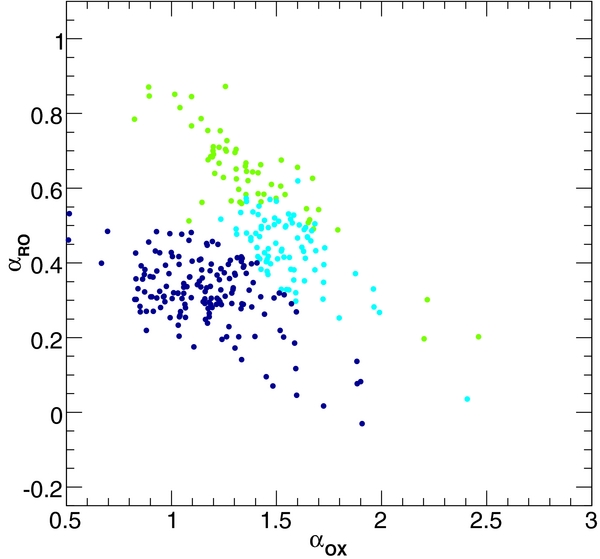
Figure 7. αro plotted against αox for BL Lac objects. Green: LSPs, light blue: ISPs, and dark blue: HSPs. The overlap of sources with different classes in this plane is due to the redshift correction applied to νSpeak (determined in the rest frame).
Download figure:
Standard image High-resolution imageThe X-ray flux is plotted against the radio flux in Figure 8. As in 1LAC, we see that the FSRQs (essentially all of the LSP type) and HSPs (all BL Lac objects) are clearly divided. This plot supports our method to classify the sources using multifrequency properties to estimate synchrotron-peak frequency.

Figure 8. X-ray flux vs. radio flux for blazars in the Clean Sample. Red: FSRQs, green: LSP-BL Lac objects, light blue: ISP-BL Lac objects, and dark blue: HSP-BL Lac objects.
Download figure:
Standard image High-resolution image5. THE SECOND LAT AGN CATALOG (2LAC)
The 2LAC catalog includes all sources with a significant detection over the two-year time period. Sources with only sporadic activity will be missing if they do not make the TS > 25 cut as computed over the full time span.
5.1. 2LAC Population Census
Table 5 presents the breakdown of sources by type for the entire 2LAC, the Clean Sample, and the low-latitude sample. The entire 2LAC includes 360 FSRQs, 423 BL Lac objects, 204 blazars of unknown type, and 30 other AGNs. Of the 373 unassociated 1FGL sources located at |b| > 10°, 107 are now firmly associated with AGNs and listed in the 2LAC. Interestingly, 84 of these were predicted to be AGNs in Ackermann et al. (2011a). In the following, only the Clean Sample is considered in tallies and figures. The Clean Sample comprises 886 sources in total, 395 BL Lac objects, 310 FSRQs, 157 sources of unknown type, 22 other AGNs, and 2 starburst galaxies. For BL Lac objects, 302 (76% of the total) have an SED classification (i.e., 93 sources cannot be classified for lack of archival data), with HSPs representing the largest subclass (53% of SED-classified sources), ISPs the second largest (27%), and LSPs the smallest subclass (20%, see Figure 6). FSRQs with SED classification (224/310 = 72%) are essentially all LSPs (99%).
Table 5. Census of Sources
| AGN Type | Entire 2LAC | 2LAC Clean Samplea | Low-lat Sample |
|---|---|---|---|
| All | 1017 | 886 | 104 |
| FSRQ | 360 | 310 | 19 |
| LSP | 246 | 221 | 7 |
| ISP | 4 | 3 | 2 |
| HSP | 2 | 0 | 0 |
| No classification | 108 | 86 | 10 |
| BL Lac | 423 | 395 | 16 |
| LSP | 65 | 61 | 3 |
| ISP | 82 | 81 | 3 |
| HSP | 174 | 160 | 5 |
| No classification | 102 | 93 | 5 |
| Blazar of unknown type | 204 | 157 | 67 |
| LSP | 24 | 19 | 10 |
| ISP | 13 | 11 | 3 |
| HSP | 65 | 53 | 13 |
| No classification | 102 | 74 | 41 |
| Other AGNs | 30 | 24 | 2 |
Note.a Sources with single counterparts and without analysis flags. See Section 5 for the definitions of this sample.
Download table as: ASCIITypeset image
Figure 9 shows the locations of the 2LAC sources. Some relative voids are present, the most prominent centered on (l, b) = (− 45°, −45°) reflecting a relative lack of counterparts in the BZCAT catalog at that location. More generally, the observed anisotropy is mainly governed by the non-uniformity of the counterpart catalogs. A difference in the numbers of sources between the northern and the southern Galactic hemispheres is clearly visible for BL Lac objects in Figure 9. This conclusion is confirmed in Figure 10 displaying the Galactic latitude distributions for FSRQs and BL Lac objects and blazars of unknown type. While the FSRQs show an approximately isotropic distribution,71 only 40% of the total number of BL Lac objects are found in the southern Galactic hemisphere (152 at b < −10°, 243 at b > 10°). At least approximately 100 other 2FGL sources at b < −10° are thus expected to be BL Lac blazars. Some of them fall into the category blazars of unknown type, which are indeed found to be more numerous at b < −10° than at b > 10° (97 versus 60), but a large fraction of these BL Lac objects obviously remain unassociated 2FGL sources.

Figure 9. Locations of the sources in the Clean Sample. Red: FSRQs, blue: BL Lac objects, magenta: non-blazar AGNs, and green: AGNs of unknown type.
Download figure:
Standard image High-resolution image
Figure 10. Galactic latitude distributions of FSRQs (top) and BL Lac objects (middle) and sources of unknown type (bottom) from the Clean Sample.
Download figure:
Standard image High-resolution imageThe comparison of the results inferred from the 1LAC and 2LAC enables the following observations.
- 1.The 2LAC Clean Sample includes 287 more sources than the 1LAC Clean Sample, i.e., a 48% increase. Of these, 234 were not present in 1FGL (58 FSRQs, 65 BL Lac objects, 108 blazars of unknown type, 3 non-blazar objects); a total of 116 sources were present in 1FGL but not included in the 1LAC Clean Sample for various reasons (their associations were not firm enough, they had more than one counterpart or were flagged in the analysis).
- 2.The fraction of FSRQs has dropped from 41% to 35% between the 1LAC and the 2LAC. The number of 2LAC Clean Sample FSRQs has increased by 22% relative to the 1LAC Clean Sample.
- 3.The fraction of BL Lac objects has remained about constant (∼45% for both 1LAC and 2LAC). The number of 2LAC Clean Sample BL Lac objects has increased by 42% relative to the 1LAC Clean Sample.
- 4.The fraction of sources with unknown type has increased fairly dramatically between the two catalogs (from 8% to 18%), in part due to the improved association procedure. The number of these sources in the 2LAC Clean Sample has increased by more than a factor of three relative to that in the 1LAC Clean Sample.
- 5.The overall fraction of FSRQs and BL Lac objects without SED classification has increased from 25% to 32%: 155 sources in the Clean Sample are without optical magnitude while 227 are without X-ray flux.
- 6.Out of 599 sources in the 1LAC Clean Sample, a total of 45 sources (listed in Table 6) are missing in the full 2LAC sample, most of them due to variability effects. A few others are present in 2FGL but with shifted positions, ruling out the association with their former counterparts. The significances reported in the 1LAC for these 45 sources are relatively low (Figure 11).

Figure 11. Significance reported in the 1FGL for 1LAC sources missing in the 2LAC. The 1FGL detection threshold is 4.05, corresponding to TS = 25.
Download figure:
Standard image High-resolution imageTable 6. 1LAC Sources Missing in 2LAC
| 1FGL Source Name | 1LAC Counterpart Name | R.A. | Decl. | Optical Class | SED Class | Redshift | 1LAC | 1LAC | 1LAC | Flags |
|---|---|---|---|---|---|---|---|---|---|---|
| (°) | (°) | Note | Clean | Prob | ||||||
| J0013.7−5022 | BZB J0014−5022 | 3.54675 | −50.37575 | BLL | HSP | ... | S | Y | 1.00 | C |
| J0019.3+2017 | PKS 0017+200 | 4.90771 | 20.36267 | BLL | LSP | ... | S | Y | 0.99 | C |
| J0041.9+2318 | PKS 0039+230 | 10.51896 | 23.33367 | FSRQ | ... | 1.426 | S | Y | 0.98 | C |
| J0202.1+0849 | RX J0202.4+0849 | 30.61000 | 8.82028 | BLL | LSP | ... | S | Y | 0.99 | C |
| J0208.6+3522 | BZB J0208+3523 | 32.15913 | 35.38686 | BLL | HSP | 0.318 | S | Y | 1.00 | C |
| J0305.0−0601 | CRATES J0305−0607 | 46.25238 | −6.12819 | BLL | ... | ... | S | Y | 0.95 | NC, V |
| J0308.3+0403 | NGC 1218 | 47.10927 | 4.11092 | AGN | ... | 0.029 | S | Y | 0.98 | C |
| J0343.4−2536 | PKS 0341−256 | 55.83138 | −25.50480 | FSRQ | LSP | 1.419 | S | Y | 0.97 | C |
| J0422.1+0211 | PKS 0420+022 | 65.71754 | 2.32414 | FSRQ | LSP | 2.277 | S | Y | 0.86 | NC, V |
| J0457.9+0649 | 4C +06.21 | 74.28212 | 6.75203 | FSRQ | LSP | 0.405 | S | Y | 0.84 | UnA |
| J0622.3−2604 | CRATES J0622-2606 | 95.59888 | −26.10767 | ... | ... | ... | S | Y | 0.99 | S |
| J0625.9−5430 | CGRaBS J0625−5438 | 96.46771 | −54.64739 | FSRQ | LSP | 2.051 | S | Y | 0.99 | BC |
| J0626.6−4254 | CRATES J0626−4253 | 96.53292 | −42.89219 | ... | ... | ... | S | Y | 0.89 | CC |
| J0645.5+6033 | BZU J0645+6024 | 101.25571 | 60.41175 | AGN | ... | 0.832 | S | Y | 0.87 | UnA |
| J0722.3+5837 | BZB J0723+5841 | 110.80817 | 58.68844 | BLL | HSP | ... | S | Y | 0.95 | NC, V |
| J0809.4+3455 | B2 0806+35 | 122.41204 | 34.92700 | BLL | HSP | 0.082 | S | Y | 0.99 | C |
| J0835.4+0936 | CRATES J0835+0937 | 128.93008 | 9.62167 | BLL | ... | ... | S | Y | 0.96 | NC, V |
| J0842.2+0251 | BZB J0842+0252 | 130.6063 | 2.88131 | BLL | HSP | 0.425 | S | Y | 0.99 | BC |
| J0850.2+3457 | RX J0850.6+3455 | 132.65083 | 34.92305 | BLL | ISP | 0.149 | S | Y | 0.99 | C |
| J0952.2+3926 | BZB J0952+3936 | 148.06129 | 39.60442 | BLL | HSP | ... | S | Y | 0.82 | NC, V |
| J1007.0+3454 | BZB J1006+3454 | 151.73527 | 34.91255 | BLL | HSP | ... | S | Y | 1.00 | NC, V |
| J1119.5−3044 | BZB J1119−3047 | 169.91458 | −30.78894 | BLL | HSP | 0.412 | S | Y | 1.00 | C |
| J1220.2+3432 | CGRaBS J1220+3431 | 185.03454 | 34.52269 | BLL | ISP | ... | S | Y | 1.00 | C |
| J1226.8+0638 | BZB J1226+0638 | 186.68428 | 6.64811 | BLL | HSP | ... | S | Y | 0.99 | C |
| J1253.7+0326 | CRATES J1253+0326 | 193.44588 | 3.44178 | BLL | HSP | 0.065 | S | Y | 0.99 | C |
| J1331.0+5202 | CGRaBS J1330+5202 | 202.67750 | 52.03761 | AGN | ... | 0.688 | S | Y | 0.99 | C |
| J1341.3+3951 | BZB J1341+3959 | 205.27127 | 39.99595 | BLL | HSP | 0.172 | S | Y | 0.93 | C |
| J1422.2+5757 | 1ES 1421+582 | 215.66206 | 58.03208 | BLL | HSP | ... | S | Y | 0.95 | C |
| J1422.7+3743 | CLASS J1423+3737 | 215.76921 | 37.62516 | BLL | ... | ... | S | Y | 0.90 | S |
| J1442.1+4348 | CLASS J1442+4348 | 220.52979 | 43.81020 | BLL | ... | ... | S | Y | 0.99 | CC |
| J1503.3+4759 | CLASS J1503+4759 | 225.94999 | 47.99195 | BLL | LSP | ... | S | Y | 0.96 | UnA |
| J1531.8+3018 | BZU J1532+3016 | 233.00929 | 30.27468 | BLL | HSP | 0.065 | S | Y | 0.99 | C |
| J1536.6+8200 | CLASS J1537+8154 | 234.25036 | 81.90862 | ... | ... | ... | S | Y | 0.82 | CC |
| J1616.1+4637 | CRATES J1616+4632 | 244.01571 | 46.54033 | FSRQ | ... | 0.95 | S | Y | 0.96 | C |
| J1624.7−0642 | 4C −06.46 | 246.13717 | −6.83047 | ... | ... | ... | S | Y | 0.94 | NC |
| J1635.4+8228 | NGC 6251 | 248.13325 | 82.53789 | AGN | ... | 0.025 | S | Y | 0.88 | O |
| J1735.4−1118 | CRATES J1735−1117 | 263.86325 | −11.29292 | ... | ... | ... | S | Y | 1.00 | C |
| J1804.1+0336 | CRATES J1803+0341 | 270.9845 | 3.68544 | FSRQ | ... | 1.42 | S | Y | 0.95 | BC |
| J1925.1−1018 | CRATES J1925−1018 | 291.26333 | −10.30344 | BLL | ... | ... | S | Y | 1.00 | S |
| J2006.6−2302 | CRATES J2005−2310 | 301.48579 | −23.17417 | FSRQ | LSP | 0.833 | S | Y | 0.91 | UnA |
| J2008.6−0419 | 3C 407 | 302.10161 | −4.30814 | AGN | ... | 0.589 | S | Y | 0.99 | NC, V |
| J2025.9−2852 | CGRaBS J2025−2845 | 306.47337 | −28.76353 | ... | LSP | ... | S | Y | 0.97 | C |
| J2117.8+0016 | CRATES J2118+0013 | 319.57250 | 0.22133 | FSRQ | ... | 0.463 | S | Y | 0.91 | C |
| J2126.1−4603 | PKS 2123−463 | 321.62846 | −46.09633 | FSRQ | ... | 1.67 | S | Y | 0.98 | S |
| J2322.3−0153 | PKS 2320−021 | 350.76929 | −1.84669 | FSRQ | ... | 1.774 | S | Y | 0.84 | C |
Notes. C = Confirmed 1FGL sources; NC = not confirmed 1FGL sources (see Abdo et al. 2011a); BC = 1FGL sources confirmed by the 11 m binned likelihood analysis; S = the 1FGL source was split/resolved in one or more seeds; O = overlapping θ99.9 error regions with one or more seeds; V = variable source visible only in the first 11 months; UnA = while the γ-ray source is in 2FGL, it is now unassociated due to the displacement of the γ-ray centroid, CC = while the γ-ray source is in 2FGL, its counterpart has changed due to the displacement of the γ-ray centroid.
Download table as: ASCIITypeset image
These findings point to a need for more multiwavelength data, in particular in the optical and X-ray bands, enabling better classification and characterization of the γ-ray-loud blazars.
5.2. Non-blazar Objects and Misaligned AGNs
Non-blazar γ-ray AGNs are those not classified as FSRQs, BL Lac objects, or as blazars of unknown/uncertain type, and constituted a small fraction of sources in the 1LAC (∼4% in the Clean Sample). In the 2LAC, this fraction is similarly small (∼3%). Among these AGNs are radio galaxies, which have emerged as a γ-ray source population due to the Fermi-LAT (e.g., Abdo et al. 2009c, 2009d, 2010g). The 2LAC contains in particular two new radio galaxies—Centaurus B and Fornax A, associated with 2FGL J1346.6−6027 and 2FGL J0322.4−3717, respectively. The LAT detects extended emission from Centaurus A (Abdo et al. 2010d), and this source is modeled with a extended spatial template in 2FGL. Cheung (2007) and Georganopoulos et al. (2008) predicted that the radio lobes of Fornax A might be seen as extended sources in the LAT, though to date no extension has been detected. In this context we also note that the position of the 2FGL source associated with the large radio galaxy NGC 6251 (∼12 in angular extent), 2FGL J1629.4+8236, is shifted toward the western radio lobe with respect to the 1FGL source position (1FGL J1635.4+8228).
The source 2FGL J0316.6+4119 is associated with the head–tail radio galaxy IC 310, whose spectrum extends up to TeV energies and was discovered with the LAT (Neronov et al. 2010) and with MAGIC (Aleksić et al. 2010). Missing from the 2LAC/2FGL are three radio galaxies reported previously—1FGL J0308.3+0403 and 1FGL J0419.0+3811, associated with 3C 78 (NGC 1218) and 3C 111, respectively (Abdo et al. 2010m), and 3C 120 (Abdo et al. 2010g). In the cases of 3C 111 and 3C 120 this may be due to the γ-ray emission being variable (Kataoka et al. 2011) and the analysis being complicated by their relatively low Galactic latitudes (b = −88 and b = −274, respectively). The 1FGL J0308.3+0403/3C 78 source is confirmed but at a significance level lower than the TS = 25 threshold for inclusion in the 2FGL catalog (see Table 7 of Abdo et al. 2011a).
Nearby AGNs with dominant γ-ray-emitting starburst components were detected in the first year of LAT observations: M 82 and NGC 253 (Abdo et al. 2010c) and NGC 1068 and NGC 4945 (Lenain et al. 2010). A study on star-forming galaxies observed with the LAT has been carried out (Ackermann et al. 2011d). The low-probability association of 1FGL J1307.0−4030 with the nearby Seyfert galaxy ESO 323−G77 is confirmed with 2FGL J1306.9−4028, with a probability of 0.8, just above the threshold. The low-probability (65%) association of 1FGL J2038.1+6552 with NGC 6951 in the 1LAC is not confirmed—instead, the γ-ray source in this vicinity, 2FGL J2036.6+6551, is now associated with the blazar CLASS J2036+6553. Finally, one new Seyfert association of note is NGC 6814 to 2FGL J1942.5−1024 with a probability of 0.91 for its radio–γ-ray match. LAT studies of other nearby Seyfert galaxies have so far resulted only in upper limits (Ackermann et al. 2011c). We conclude that such radio-quiet sources do not emit strongly in γ-rays.
No new radio-loud narrow-line Seyfert 1 galaxies beyond those four detected in the first year (Abdo et al. 2009f, 2009g) were found, although such objects can be highly variable in γ-rays and one such example (SBS 0846+513) has been recently detected while flaring (Donato & Perkins 2011), though it does not make it into 2FGL/2LAC as it was too faint during the first 24 months of LAT operation.
5.3. Low-latitude AGNs
Diffuse radio emission, Galactic point sources, and heavy optical extinction make the low-latitude sky a difficult region for AGN studies, and catalogs of AGNs and AGN candidates often avoid it partially or entirely. However, we are able to make associations with 104 low-latitude AGNs (while about 210 AGNs would be expected in this region from the high-latitude observations if the LAT sensitivity remained the same); these are presented in Table 4. Although the associations are considered valid, these sources have, in general, been studied much less uniformly and much less thoroughly than the high-latitude sources at virtually all wavelengths, so we do not include them as part of the Clean Sample in order to keep them from skewing any of our analyses of the overall γ-ray AGN population.
5.4. Notes on Individual Sources
As in the 1LAC, we provide additional notes on selected sources. Associations discussed in the previous subsection (Section 5.2) on non-blazars and misaligned AGNs are not repeated.
2FGL J0319.8+4130. This is the LAT source associated with the radio galaxy NGC 1275 discovered early in the Fermi mission (Abdo et al. 2009c). During the first two years of LAT operation, the MeV/GeV emission is variable with significant spectral changes at >GeV energies (Kataoka et al. 2010; Brown & Adams 2011).
2FGL J0339.2−1734. As noted in the 1LAC, the optical spectrum of the associated AGN source PKS 0336−177 is not easily classified as BL Lac object or FSRQ.
2FGL J0523.0−3628. The radio source associated with this EGRET γ-ray source is PKS 0521−36, which has historically been classified as a BL Lac object because of its optically variable continuum (Danziger et al. 1979). However, its spectrum obtained in our optical follow-up program did not enable a clear classification. It is thus flagged as a generic AGN.
2FGL J0627.1−3528. This LAT source was associated with PKS 0625−35, classified as a radio galaxy, but with BL Lac object characteristics in the optical as discussed in Abdo et al. (2010g).
2FGL J0840.7+1310. This LAT source was associated with 3C 207, classified as an SSRQ, and was analyzed in more detail in Abdo et al. (2010g).
2FGL J0847.0−2334. This source is associated with CRATES J0847−2337 and has been classified as a "galaxy" in our optical follow-up program.
2FGL J0903.6+4238. This radio source, S4 0900+42, was selected by Fanti et al. (2001) in a search for candidate compact steep spectrum radio sources. It was then rejected because—interestingly—deeper observations revealed an extended (>40 kpc) low-frequency radio structure. In the lack of an optical spectrum, this source could then be considered as a candidate misaligned AGN.
2FGL J0904.9−5735. The associated radio source, PKS 0903−57, was classified as a Seyfert 1 galaxy at z = 0.695 by Thompson et al. (1990). Its spectrum obtained in our optical follow-up program did not enable a clear classification.
2FGL J0942.8−7558. The LAT source was associated with the radio source, PKS 0943−76, and studied in Abdo et al. (2010g). The photometric redshift of the radio source is z = 0.26 and it appears to have an FR II morphology (Burgess & Hunstead 2006).
2FGL J1230.8+1224. This LAT source is associated with the radio galaxy M87, discovered initially in the first year LAT data (Abdo et al. 2009d). No significant variability is observed with the LAT within the first two years of observations (see Abramowski et al. 2011b).
2FGL J1256.5−1145. The associated source is CRATES J1256−1146 (z = 0.058) whose spectrum obtained in our optical follow-up program did not enable a clear classification.
2FGL J1329.3−0528. The associated AGN, 1RXS 132928.0−053132, is not a known radio emitter (e.g., in the NVSS survey).
2FGL J1641.0+1141. The associated AGN, CRATES J1640+1144, was noted in the 1LAC as simply a "galaxy." Its spectrum obtained in our optical follow-up program did not enable a clear classification.
2FGL J1647.5+4950. The associated AGN is SBS 1646+499, already noted in the 1LAC as characterized as a nearby (z = 0.047) late-type galaxy. It is a BZU type in BZCAT. Its spectrum obtained in our optical follow-up program did not enable a clear classification.
2FGL J1829.7+4846. This LAT source was associated with 3C 380, classified as an SSRQ and was analyzed in more detail in Abdo et al. (2010g).
2FGL J2250.8−2808. The LAT detected a flare from this object in 2009 March (Koerding 2009). The associated flat-spectrum radio source, PMN J2250−2806, has a redshift z = 0.525. Its spectrum obtained in our optical follow-up program did not enable a clear classification.
6. PROPERTIES OF THE 2LAC SOURCES
6.1. Redshift Distributions
The redshift distributions of the various classes are shown in Figure 12. They are very similar to those obtained with 1LAC. The distribution peaks around z = 1 for FSRQs (Figure 12 top) and extends to z = 3.10. This distribution contrasts with that of sources observed in the Burst Alert Telescope catalog (Ajello et al. 2009) where 40% of FSRQs have a redshift greater than 2. The distribution peaks at a lower redshift for BL Lac objects (Figure 12, middle). Note that 56% of the BL Lac objects have no measured redshifts. The fraction of BL Lac objects having a measured redshift is higher for sources with an SED-based classification. This fraction is essentially constant for the different subclasses 49%, 49%, 54% for LSPs, ISPs, HSPs, respectively. Figure 12 bottom shows the redshift distributions for the different subclasses of BL Lac objects. These distributions gradually extend to lower redshifts as the location of the synchrotron peak shifts to higher frequency, i.e., from LSPs to HSPs.

Figure 12. Redshift distributions for FSRQs (top), BL Lac objects (middle), LSP-BL Lac objects (bottom, green), ISP-BL Lac objects (bottom, light blue), and HSP-BL Lac objects (bottom, dark blue).
Download figure:
Standard image High-resolution imageThe redshift distributions of FSRQs and BL Lac objects are compared in Figure 13 to the corresponding distributions for the sources obtained by cross-correlating the seven-year WMAP catalog (Gold et al. 2011) with BZCat, using a correlation radius of 11' (thus selecting 339 sources of a total of 471). Good agreement is observed for FSRQs. The agreement between the 2LAC and WMAP distributions of BL Lac objects is more marginal, but the low number of BL Lac objects with measured redshifts in the WMAP sample (29 sources) prevents us from drawing definite conclusions. Note that all BL Lac objects in the WMAP catalog are detected by the LAT, while only 50% (130 of 260) of the WMAP FSRQs fulfill this condition.

Figure 13. Comparison between redshift distributions for blazars in the 2LAC Clean Sample (solid) and the 5 year WMAP complete sample (dashed). Top: FSRQs. Bottom: BL Lac objects.
Download figure:
Standard image High-resolution image6.2. Flux and Photon Spectral Index Distributions
The photon index is plotted versus the mean flux (E > 100 MeV) in Figure 14, along with an estimate of the flux limit. The flux limit strongly depends on the photon index as harder sources are easier to discriminate against the background, which is due to the narrowing of the point-spread function (PSF) of the LAT with increasing energy and to the relative softness of the diffuse Galactic γ-ray emission. In contrast, the limit in energy flux above 100 MeV is almost independent of the photon index as illustrated in Figure 15.

Figure 14. Photon index vs. flux above 100 MeV for blazars in the Clean Sample. Red: FSRQs, blue: BL Lac objects, magenta: non-blazar AGNs, and green: AGNs of unknown type.
Download figure:
Standard image High-resolution image
Figure 15. Photon index vs. energy flux above 100 MeV. Red: FSRQs, blue: BL Lac objects. The curve represents the approximate detection limit.
Download figure:
Standard image High-resolution imageThe photon index distributions are given in Figure 16 for the different classes of blazars. The now well-established spectral difference in the LAT energy range between FSRQs and BL Lac objects, with a moderate overlap between the distributions (Abdo et al. 2009a, 2010m) is still present. The index distribution of sources with unknown types spans a wider range than those of FSRQs and BL Lac objects separately. Assuming that the class of sources with unknown types is entirely made up of FSRQs and BL Lac objects lacking classification, each with the same photon index distributions as the classified sources, FSRQs and BL Lac objects would contribute about equally to this component.
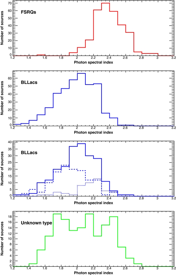
Figure 16. Photon index distributions. Top: FSRQs. Second from top: BL Lac objects. Second from bottom: BL Lac objects without redshift (solid), BL Lac objects with z < 0.5 (dashed), BL Lac objects with z > 0.5 (dotted). Bottom: blazars of unknown type.
Download figure:
Standard image High-resolution imageThe photon index is plotted versus the frequency of the synchrotron peak in Figure 17. A relatively strong correlation between these two parameters, again reported earlier (Abdo et al. 2009a, 2010m) is observed. Strong conclusions regarding the HSP-BL Lac object outliers (e.g., 2FGL J1213.2−2616/ RBS 1080 and 2FGL J1023.6+2959/RX J1023.6+3001 with Γ = 2.4 and Γ = 1.2, respectively) should not be made as these sources are very faint and are significantly detected at best in only one energy band. In order to make a meaningful comparison between the photon index distributions for different classes, it is advantageous to use the flux-limited sample, i.e., sources with Flux[E > 100 MeV] > 1.5 × 10⁻⁸ photons cm−2 s−1, which is free of the bias arising from the photon index dependence of the flux limit (Figure 14). The resulting photon index distributions are shown in Figure 18. The distribution mean values and rms are 2.42 ± 0.17, 2.17 ± 0.12, 2.13 ± 0.14, 1.90 ± 0.17 for FSRQs, LSP-BL Lac objects, ISP-BL Lac objects, HSP-BL Lac objects, respectively. For orientation, the mean values in the significance-limited sample are 2.39, 2.14, 2.09, 1.81 for FSRQs, LSP-BL Lac objects, ISP-BL Lac objects, HSP-BL Lac objects, respectively. No significant dependence of the photon index on redshift is observed if blazar subclasses are considered separately, as illustrated in Figure 19, corroborating the conclusion drawn with 1LAC. Note that the region populated by LSP-BL Lac objects in the (redshift, Γ) plane overlaps but does not strictly coincide with that populated by FSRQs. The FSRQ with z = 2.941 and Γ = 1.59 ± 0.23 is 2FGL J0521.9+0108/CRATES J0522+0113, which, while having a definite classification, exhibits a complex optical spectrum. This source is located in the Orion region, where uncertainties in our knowledge of the Galactic diffuse emission can affect the determination of the source photon spectral index. The three photon index distributions for BL Lac objects with z < 0.5 (mostly HSPs), with z > 0.5 (mostly LSPs), and for BL Lac objects without redshifts are compared in Figure 16. The distribution of BL Lac objects without redshifts is markedly different from the two other distributions and thus does not favor any conclusions concerning the actual redshift distributions of these blazars.

Figure 17. Photon index vs. frequency of the synchrotron peak νSpeak. Red: FSRQs, green: LSP-BL Lac objects, light blue: ISP-BL Lac objects, and dark blue: HSP-BL Lac objects.
Download figure:
Standard image High-resolution image
Figure 18. Photon spectral index distributions for the different blazar classes for sources in the Clean Sample with F[E > 100 MeV] > 1.5 × 10⁻⁸ photons cm−2 s−1.
Download figure:
Standard image High-resolution image
Figure 19. Photon spectral index vs. redshift. Red: FSRQs, green: LSP-BL Lac objects, light blue: ISP-BL Lac objects, and dark blue: HSP-BL Lac objects.
Download figure:
Standard image High-resolution imageThe time-averaged, mean flux distributions for FSRQs and BL Lac objects are compared in Figure 20(a). As suggested by Figure 14, the fluxes of the FSRQs extend to higher values than do BL Lac objects, but FSRQs have a higher detection flux limit due to their spectral softness. For sources showing significant variability, the monthly peak flux distributions are compared in Figure 20(b). These distributions are more similar for the two blazar classes. The peak flux is plotted as a function of mean flux in Figure 20(c), and the distribution of peak flux over mean flux ratio is given in Figure 20(d). Larger flux ratios are observed for FSRQs. Variability is discussed further in Section 6.5.

Figure 20. (a) Mean flux distributions. Red: FSRQs, blue: BL Lac objects. (b) Peak flux distributions. (c) Peak flux vs. mean flux. (d) Peak flux over mean flux ratio.
Download figure:
Standard image High-resolution image6.3. Comparison of 2LAC and 1LAC Fluxes
Photon flux distributions from 1LAC and 2LAC are displayed in Figure 21. The top two panels show the 1LAC fluxes and 2LAC fluxes for sources present in both 1LAC and 2LAC. As expected the 2LAC distribution is broader than the 1LAC distribution, especially at the low-flux end. The bottom two panels represent the 1LAC flux distribution for the 45 missing 1LAC sources and the 2LAC flux distribution for the 250 newly detected 2LAC sources in the Clean Sample. The high-flux end of these distributions look alike, which can presumably arise from the facts that a similar pool of sources (1) were comparatively bright during the first 11 months and then faded away, or (2) have brightened during the last 13 months spanned by the 2LAC while being faint during the 1LAC period. Of course, the low-flux ends of the two distributions are different as the new 2LAC sources include sources fainter than the 1LAC detection limit.

Figure 21. Distributions of flux above 100 MeV. The top and second panels show the 1LAC fluxes and 2LAC fluxes for sources in both 1LAC and 2LAC, respectively. The third panel shows 1LAC fluxes of 1LAC sources missing in the 2LAC. The bottom panel displays the 2LAC fluxes for new sources in the 2LAC absent in the 1LAC.
Download figure:
Standard image High-resolution image6.4. Energy Spectra
First observed for 3C 454.3 (Abdo et al. 2009b) early in the Fermi mission, a significant curvature in the energy spectra of many bright FSRQs and some bright LSP-/ISP-BL Lac objects is now a well-established feature (Abdo et al. 2010k, 2010m). The break energy obtained from a broken power-law fit has been found to be remarkably constant as a function of the flux, at least for 3C 454.3 (Abdo et al. 2011b). Several explanations have been proposed to account for this feature, including γγ attenuation from He ii line photons (Poutanen & Stern 2010), intrinsic electron spectral breaks (Abdo et al. 2009b), Ly α scattering (Ackermann et al. 2010), and hybrid scattering (Finke & Dermer 2010).
Although broken power-law (BPL) functions have been found to better reproduce most curved blazar energy spectra, the LogParabola function (Section 2) has been selected here since it has only one more degree of freedom with respect to a power law, convergence of spectral fits is easier than for BPL and the function decreases more smoothly at high energy than a power law with exponential cutoff form. Physical arguments supporting the use of a LogParabola function have been presented in Tramacere et al. (2011).
The spectral curvature is characterized by the parameter  , equal to
  , where TScurve is defined in Section 2 and c is a source-dependent correction factor accounting for systematic effects (see Abdo et al. 2011a, for details).
  is plotted as a function of TS in Figure 22. For TS > 1000, most FSRQs have large
  , while BL Lac objects exhibit a variety of behaviors. As mentioned earlier, LogParabola results were retained for sources with TScurve > 16 (corresponding to
  4). The LogParabola parameter β is plotted as a function of the flux in Figure 23 for the 57 FSRQs and 12 BL Lac objects in the Clean Sample with TScurve > 16. The average β is significantly lower for BL Lac objects than for FSRQs (0.11 ± 0.02 versus 0.18 ± 0.02, respectively), possibly due to the fact that different regions of the inverse Compton peak (assuming a leptonic scenario) are probed in the LAT energy band.

Figure 22.  , defined as the square root of TScurve times a correction factor accounting for systematic effects, vs. TS. Red: FSRQs, blue: BL Lac objects.
Download figure:
Standard image High-resolution image
Figure 23. LogParabola parameter β plotted as a function of flux above 100 MeV. Red: FSRQs, blue: BL Lac objects.
Download figure:
Standard image High-resolution imageThe 12 BL Lac objects comprise 7 LSPs, 3 ISPs, 1 HSP, and 1 BL Lac object lacking SED classification. The HSP is BZB J1015+4926 (GB 1011+496), the SED of which has a maximum at a few GeV. The flux distributions for these sources are compared to the overall distributions in Figure 24, and are seen to confirm the trend observed in Figure 22.

Figure 24. Top: flux distribution of sources exhibiting significant spectral curvature (black, dashed) compared to the full distribution (red) for FSRQs. Bottom: flux distribution of sources exhibiting significant spectral curvature (green) compared to the full distribution (blue) for BL Lac objects.
Download figure:
Standard image High-resolution image6.5. Variability
Variability at all timescales is one of the distinctive properties of blazars. Since launch, detections by the Fermi-LAT of γ-ray activity from 81 flaring blazars have been reported in Astronomer's Telegrams (ATels). Four of them are not listed in the 2LAC since they did not pass the TS = 25 cut for inclusion in the 2FGL: SBS 0846+513, PMN J1123−6417 (at b = 30), PMN J1913−3630, and PKS 1915−458.
Two-year light curves with monthly binning were obtained as part of the 2FGL catalog. The large bin width leads to a substantial smoothing of the light curves for the brightest blazars, for which peak fluxes may be much higher than the one-month average fluxes reported here. A more extensive analysis using higher-resolution light curves, thus containing richer temporal information will be presented elsewhere. Nevertheless these light curves constitute the largest set ever produced in the γ-ray band, allowing variability analysis on a wide sample of blazars. In this section, we will give an overview of the variability properties for the sources in the 2LAC Clean Sample. This includes the detection of variability via the LAT γ-ray variability index, a measure of the γ-ray variability duty cycle and a derivation of population variability characteristics from the discrete autocorrelation function, DACF, first-order structure function, SF, and from power density spectra, PDS. DACF (see, e.g., Edelson & Krolik 1988; Hufnagel & Bregman 1992), SF (see, e.g., Simonetti et al. 1985; Smith et al. 1993; Lainela & Valtaoja 1993; Paltani et al. 1997), and PDS (Vaughan et al. 2003) are methods providing insights into fluctuation modes, characteristic timescales, and flavors of the variability modes in the γ-ray monthly bin light curves. A short description of these three analysis methods is given in Abdo et al. (2010i).
The variability index TSvar, which is described in Section 2, is plotted as a function of the relative flux uncertainty in Figure 25. The relative flux uncertainty, computed with a fixed photon index (see Section 3.6 of Abdo et al. 2011a), reflects the photon statistics. This parameter allows meaningful comparisons between sources with different fluxes and photon indices. Figure 25 illustrates the fact that for a source to be labeled as variable on the basis of its variability index it must be both intrinsically variable and sufficiently bright. All very bright sources, including both FSRQs and BL Lac objects are found to be variable at a confidence level greater than 99%, depicted by the line at TSvar > 41.6 in Figure 25. At a given relative flux uncertainty, BL Lac objects have on average lower TSvar than FSRQs.

Figure 25. Variability index vs. relative flux uncertainty. Red: FSRQs, blue: BL Lac objects. The dashed line corresponds to the 99% confidence level for a source to be variable.
Download figure:
Standard image High-resolution imageA total of 224 FSRQs (out of 310), 91 BL Lac objects (out of 395) and 33 sources of unknown type (out of 157) are variable at a confidence level greater than 99%. Thus, 348 blazars of the 2LAC Clean Sample fulfill this condition, while there were only 189 in the 1LAC Clean Sample. Figure 26 shows the variability index versus synchrotron-peak position. Only a small fraction of the HSP-BL Lac objects detected by the LAT shows significant variability (27 out of 160), substantially less than LSP-BL Lac objects (25 out of 61), and ISP-BL Lac objects (30 out of 81). The photon indices of variable FSRQs and BL Lac objects are shown in Figure 27 versus the normalized excess variance (Vaughan et al. 2003). The plot reveals a trend of variability with spectral index. Most variable sources have a photon index greater than 2.2. These sources are observed at energies greater than the peak energies of their SEDs, where the variability amplitude tends to be larger. The harder sources, including all but one (PKS 0301−243) of the HSPs and ISPs have normalized excess variance <0.5. The average normalized excess variance for each of the blazar classes is 0.37 ± 0.03 (FSRQs), 0.28 ± 0.07 (LSP-BL Lac objects), 0.19 ± 0.04 (ISP-BL Lac objects), and 0.20 ± 0.10 (HSP-BL Lac objects). Excluding the outlier (PKS 0301−243) the value for the HSP-BL Lac objects becomes 0.10 ± 0.03 which implies that even if significant variability is detected only in a fraction of the individual HSPs, they do, as a class, exhibit variability but at a lower level than the other classes. The variability index and normalized excess variance are also plotted against γ-ray luminosity. These are shown in Figures 28 and 29, respectively. The normalized excess variance does show a gradual increase with γ-ray luminosity for both BL Lac objects and FSRQs. The BL Lac object with low luminosity and high normalized excess variance (>1.5) is 2FGL J0217.4+0836, which underwent a flare with a Flux[E > 100 MeV] = 1.3 × 10⁻⁷ photons cm−2 s−1 flare in 2010 January.

Figure 26. Variability index vs. synchrotron-peak frequency. Red: FSRQs, green: LSP-BL Lac objects, light blue: ISP-BL Lac objects, and dark blue: HSP-BL Lac objects. The dashed line corresponds to the 99% confidence level for a source to be variable.
Download figure:
Standard image High-resolution image
Figure 27. Photon spectral index vs. normalized excess variance for sources with flux greater than 3 × 10⁻⁸ photons cm−2 s−1. Red: FSRQs, green: LSP-BL Lac objects, light blue: ISP-BL Lac objects, and dark blue: HSP-BL Lac objects.
Download figure:
Standard image High-resolution image
Figure 28. Variability index vs. γ-ray luminosity. Red: FSRQ, blue: BL Lac objects. The dashed line corresponds to the 99% confidence level for a source to be variable.
Download figure:
Standard image High-resolution image
Figure 29. Normalized excess variance vs. γ-ray luminosity. Red: FSRQs, blue: BL Lac objects.
Download figure:
Standard image High-resolution imageThe monthly binned light curves also provide information about the duty cycle of blazars at γ-ray energies. Sources are in general not detected in all one-month bins. This is illustrated in Figure 30, which shows the distribution of coverage, i.e., the fraction of months where the source was detected with TS > 4. Not surprisingly, the coverage distribution is skewed toward low values. We find that 161 FSRQs and 152 BL Lac objects have a coverage greater than 0.5. Only these sources will be considered in the variability studies presented below. We define the duty cycle as the fraction of monthly periods Nb/Ntot where the flux exceeds 〈F〉 + 1.5S + σi, where 〈F〉 is the average flux, S is the total standard deviation, and σi is the flux uncertainty of month i (Abdo et al. 2010i). These duty cycle values are shown as a function of TS in Figure 31. Bright sources with TS > 1000 essentially have all Nb/Ntot ⩾ 0.05. Simulations considering the actual TS distributions of both blazar classes were performed and showed that the measurement of Nb/Ntot for these sources was not significantly affected by measurement noise. The wider distribution in Nb/Ntot for sources with TS < 1000 is consistent with these sources having similar duty cycle as the brighter ones and only results from a lower signal-to-noise ratio.

Figure 30. Coverage distributions for BL Lac objects (blue) and FSRQs (red) in the Clean Sample.
Download figure:
Standard image High-resolution image
Figure 31. Duty cycle (defined as the fraction of monthly periods where the flux exceeds 〈F〉 + 1.5 S + σi) vs. TS for FSRQs (red) and BL Lac objects (blue).
Download figure:
Standard image High-resolution imageDACF and PDS were calculated for all sources with coverage larger than 0.5 and mean flux above 100 MeV exceeding 3 × 10⁻⁸ photons cm−2 s−1 (156 FSRQs and 59 BL Lac objects), while the SF analysis was applied to the whole Clean Sample. From each DACF a correlation timescale was estimated as the time lag of the first zero crossing of the function, computed by linear interpolation between the lag points. These observer-frame timescale estimates for both FSRQs and BL Lac objects are plotted in Figure 32 as a function of synchrotron-peak frequency for the selected sources. The timescale distribution is shown in the inset plot. Interestingly the observation that FSRQs have γ-ray correlation extending to longer timescales than BL Lac objects confirms the trend found for the LBAS sample (Abdo et al. 2009a) using weekly light curves obtained over the first 11 months of observation (Abdo et al. 2010i).

Figure 32. Observed discrete autocorrelation function (DACF) γ-ray correlation timescales vs. the source-frame synchrotron-peak frequency for the monthly light curves of the 2LAC sources having at least 50% of the 24 bins with flux detections of TS ⩾ 4. Red circles: FSRQs, blue diamonds: BL Lac objects. Inset panel: distribution of DACF γ-ray correlation timescales. Red/continuous line: FSRQs, blue/dashed line: BL Lac objects.
Download figure:
Standard image High-resolution imageThe SF, which is equivalent to the PDS of the signal but calculated in the time domain, which makes it less subject to irregular sampling, low significance bins and upper limit problems, was applied to the light curves of the entire 2LAC Clean Sample sources. Results are shown in Figure 33 where the distribution of the PDS power-law indexes evaluated in the time domain (β + 1, where β is the blind power-law slope estimated from the SF of each light curve) are reported for the FSRQs and BL Lac objects. The resulting distributions of the power-law indices appear whitened (i.e., closer to white noise with flatter SF power-law indices) because of the short extent of the time lag range investigated (from 1 to 24 months) and of the fact that a consistent subset of the 2LAC Clean Sample showed low-flux, noisy, and non-variable monthly bin light curves, when compared with the same analysis performed on the brightest and better sampled light curves of the LBAS sample (Abdo et al. 2010i). Again the distribution shows FSRQs with slightly more Brownian-like (steeper) and more scattered SF indexes, with respect to the more flicker-like (flatter) ones for BL Lac objects in agreement with what was already found for the LBAS sample (Abdo et al. 2010i).

Figure 33. Distribution of the temporal PDS power-law indexes (β + 1) for the FSRQs (red) and BL Lac objects (blue) of the 2LAC Clean Sample, evaluated in time domain using a first-order structure function (SF) analysis with blind power-law β slope estimation.
Download figure:
Standard image High-resolution imageIn Figure 34, we have plotted the average PDS for FSRQs and BL Lac objects. The power density is normalized to fractional variance per frequency unit ( rms2 I−2 day−1, where I is the average flux) and the PDS points are averaged in logarithmic frequency bins. The white noise level was estimated from the rms of the flux errors and was subtracted for each PDS. The error bars were computed as the standard error of the mean for each frequency bin. The PDS slope (power-law index) is similar for the two groups, ∼1.15 ± 0.10. This is somewhat flatter than was deduced for the very brightest sources in the LBAS sample (Abdo et al. 2010i). The difference in the height of the PDS means that the fractional variability of BL Lac objects is lower than that of FSRQs. This is in line with the LBAS results. With the PDS normalization used here, we can compute a normalized excess variance by integrating the PDS over frequency. To limit the effect of statistical noise this integration was done for frequencies up to 0.2 month−1, which also contains most of the variance. The resulting normalized excess variance for the different blazar classes is 0.44 ± 0.04 (FSRQs), 0.27 ± 0.10 (LSP-BL Lac objects), 0.19 ± 0.04 (ISP-BL Lac objects), and 0.14 ± 0.07 (HSP-BL Lac objects). The trend and values are consistent with the normalized excess variance calculated directly from the light curves as described above.

Figure 34. Power density spectrum (PDS) for bright FSRQs (red) and BL Lac objects (blue).
Download figure:
Standard image High-resolution image6.6. Highest-energy Photons
Figure 35 displays, as a function of redshift, the highest-energy photon (HEP) detected by the LAT from the 2LAC AGN sample using the Pass 7_V6 Ultraclean event selection and that is associated with the source within the 68% containment radius. Further work is being carried out to improve the capability to reconstruct event tracks and reject background at high energy (Rochester et al. 2010). In comparison to the corresponding sample based on 11 months of LAT operation (Abdo et al. 2010e), we find about a factor ∼2 more candidate photon events coming from sufficiently high redshift (z > 0.5) to probe the models of the EBL.

Figure 35. Top: maximum photon energy vs. redshift. Red: FSRQs, blue: BL Lac objects. The curves correspond to predictions for τ = 1 for different models. Bottom: same but the curves correspond to predictions for τ = 3 for different models.
Download figure:
Standard image High-resolution imagePredictions of γγ opacity curves, τγγ = 1 (top panel) and τγγ = 3 (bottom panel), for different EBL models are also shown in Figure 35. Detection of HEPs above the opacity curve predicted by a given model makes the model less likely. In the new 2LAC AGN sample, we find 30 HEP events from z > 0.5 sources beyond the τγγ = 3 regime of the Stecker et al. (2006) "baseline model," which is already severely constrained by the LAT 11 month data set (Abdo et al. 2010e). Only one event appears beyond τγγ = 3 of the Kneiske et al. (2004) "best-fit" and "high-UV" models.
None of the HEP events seems to be in strong contradiction with EBL models that are of lower photon density (e.g., Franceschini et al. 2008; Finke et al. 2010; Gilmore et al. 2009). Note, however, that we do not have redshift information for more than 50% of the 36 sources with HEPs at energies greater than 100 GeV, which can therefore not be tested against any EBL models. Apparent in Figure 12 is the clustering of HSPs at low redshifts (z ⩽ 0.2) while LSPs cover a broad redshift range up to z = 3.1. Because HSPs are intrinsically hard sources and LSPs intrinsically soft (see Figure 17), any systematic trend between redshift and spectral properties (spectral index, HEP) is unlikely to be caused by EBL absorption only. For the >500 events without an assigned source redshift, the HEP is located above ∼10 GeV in more than ∼70% of all cases. Interestingly, we found ∼4 FSRQs with HEPs that reach energies >100 GeV (4C +55.17, see McConville et al. 2011, 4C +21.35, PKS 1958−179, BZQ J1722+1013) with the latter two (at redshifts z = 0.652 and z = 0.732, respectively) displaying no significant deviation from a power-law spectrum (with indices Γ ∼ 2.4 and Γ ∼ 2.2, respectively) in the energy range of the LAT. One BL Lac object (2FGL J0428.6−3756, PKS 0426−380) at redshift z = 1.10 of LSP spectral type has also been detected at >100 GeV.
6.7. Luminosity Distributions
The γ-ray luminosity is plotted as a function of redshift in Figure 36. A Malmquist bias is readily apparent in this figure as only high-luminosity sources (mostly FSRQs) are detected at large distances. Given their γ-ray luminosity distribution, most BL Lac objects could not be detected if they were located at redshifts greater than 1.

Figure 36. Gamma-ray luminosity vs. redshift. Red: FSRQs, blue: BL Lac objects. The solid (dashed) curve represents the approximate detection limit for Γ = 1.8 (Γ = 2.2).
Download figure:
Standard image High-resolution imageFigure 37 shows photon index versus γ-ray luminosity. This correlation has been discussed in detail in the context of the "blazar divide" (Ghisellini et al. 2009). Note that since the γ-ray luminosity is derived from the energy flux and that the detection limit in energy flux is essentially independent of the photon index (Figure 15), no significant LAT-related detection bias is expected to affect this correlation. The ISP-BL Lac object outlier at Lγ ≃ 3 × 1043 erg cm−2 s−1 is 4C 04.77 (2FGL J2204.6+0442) at z = 0.027, which was classified as an AGN in 1LAC.

Figure 37. Photon index vs. γ-ray luminosity. Red: FSRQs, green: LSP-BL Lac objects, light blue: ISP-BL Lac objects, dark blue: HSP-BL Lac objects, magenta: non-blazar AGNs (circles: NLS1s, squares: misaligned AGNs, up triangles: starbursts, down triangles: other AGNs).
Download figure:
Standard image High-resolution imageFigure 38 shows photon index versus γ-ray luminosity for FSRQs (top) and BL Lac objects (bottom) separately. The Pearson correlation coefficients are −0.04 and 0.14 for FSRQs and BL Lac objects, respectively. For a given class, the correlation is very weak.

Figure 38. Photon index vs. γ-ray luminosity. Top: FSRQs. Bottom: green: LSP-BL Lac objects, light blue: ISP-BL Lac objects, and dark blue: HSP-BL Lac objects.
Download figure:
Standard image High-resolution image7. MULTIWAVELENGTH PROPERTIES OF THE 2LAC SAMPLE
In this section, we explore the properties of the 2LAC sample in the radio, optical, X-ray, and TeV bands. Table 7 gives archival fluxes in different bands for these sources. For completeness, Table 8 provides the corresponding fluxes for the low-latitude sources.
Table 7. 2LAC Sources: Flux Table (High-latitude Sources)
| 2FGL Source Name | Counterpart Name | TS | Radio Flux | X-ray Flux | USNO B1 | SDSS | αox | αro |
|---|---|---|---|---|---|---|---|---|
| (mJy) | (10−13 erg cm−2 s−1) | (V mag) | (V mag) | |||||
| J0000.9−0748* | PMN J0001−0746 | 46 | 209 | 8.10 | 17.61 | ... | 1.33 | 0.53 |
| J0001.7−4159* | 1RXS J000135.5−41551 | 45 | 12 | 11.01 | 18.97 | ... | 1.12 | 0.17 |
| J0004.7−4736* | PKS 0002−478 | 173 | 995 | 14.70 | 17.30 | ... | 1.12 | 0.67 |
| J0006.1+3821* | S4 0003+38 | 164 | 573 | 14.10 | 17.72 | ... | 1.20 | 0.65 |
| J0007.8+4713* | MG4 J000800+4712 | 326 | 61 | 14.80 | 18.28 | ... | 1.08 | 0.51 |
| J0008.7−2344 | RBS 0016 | 25 | 36 | ... | 16.64 | ... | ... | 0.42 |
| J0008.7−2344− | PKS 0005−239 | 25 | 375 | ... | 16.51 | ... | ... | 0.55 |
| J0009.0+0632− | GB6 J0009+0625 | 43 | 180 | ... | 19.49 | 19.19 | ... | ... |
| J0009.0+0632 | CRATES J0009+0628 | 43 | 247 | 13.00 | 18.70 | 18.10 | 1.17 | 0.63 |
| J0009.1+5030* | NVSS J000922+503028 | 310 | 12 | ... | 19.52 | ... | ... | ... |
| J0009.9−3206 | IC 1531 | 35 | 389 | 5.01 | 8.91 | ... | 2.78 | −0.09 |
| J0011.3+0054 | PMN J0011+0058 | 49 | 167 | 5.41 | 20.17 | 20.40 | 0.86 | 0.78 |
| J0012.9−3954* | PKS 0010−401 | 50 | 495 | ... | 18.09 | ... | ... | 0.74 |
| J0013.8+1907* | GB6 J0013+1910 | 25 | 161 | ... | 18.41 | ... | ... | 0.61 |
| J0017.4−0018* | S3 0013−00 | 38 | 1086 | 3.19 | 19.99 | 19.17 | 1.11 | 0.84 |
| J0017.6−0510* | PMN J0017−0512 | 185 | 178 | 17.40 | 18.09 | ... | 1.10 | 0.63 |
| J0018.5+2945* | RBS 0042 | 31 | 34 | 143.00 | 17.47 | ... | 0.90 | 0.36 |
| J0018.8−8154* | PMN J0019−8152 | 69 | 83 | 29.70 | 16.35 | ... | 1.32 | 0.30 |
| J0019.4−5645* | PMN J0019−5641 | 37 | 61 | ... | 20.36 | ... | ... | ... |
| J0021.6−2551* | CRATES J0021−2550 | 116 | 69 | 1.72 | 17.22 | ... | 1.63 | 0.49 |
| J0022.2−1853* | 1RXS 002209.2−185333 | 141 | 23 | 10.90 | 17.45 | ... | 1.34 | 0.32 |
| J0022.3−5141* | 1RXS 002159.2−514028 | 36 | 20 | 50.30 | 16.58 | ... | 1.15 | 0.23 |
| J0022.5+0607* | PKS 0019+058 | 391 | 340 | 2.45 | 19.51 | ... | 1.04 | 0.82 |
| J0023.2+4454* | B3 0020+446 | 76 | 141 | ... | ... | ... | ... | ... |
| J0024.5+0346* | GB6 J0024+0349 | 32 | 22 | ... | 19.81 | ... | ... | 0.61 |
Notes. * refers to sources in the Clean Sample, − refers to counterparts not given in the 2FGL catalog for source with double associations. The full table is available at http://www.asdc.asi.it/fermi2lac/.
Only a portion of this table is shown here to demonstrate its form and content. A machine-readable version of the full table is available.
Download table as: DataTypeset image
Table 8. Flux Table, Low-latitude Sources
| 2FGL Source Name | Counterpart Name | TS | Radio Flux | X-ray Flux | USNO B1 | SDSS | αox | αro |
|---|---|---|---|---|---|---|---|---|
| (mJy) | (10−13 erg cm−2 s−1) | (V mag) | (V mag) | |||||
| J0010.5+6556 | GB6 J0011+6603 | 71 | 64 | ... | 19.70 | ... | ... | ... |
| J0035.8+5951 | 1ES 0033+595 | 243 | 148 | 318.00 | 18.21 | ... | 1.01 | 0.37 |
| J0047.2+5657 | GB6 J0047+5657 | 201 | 190 | ... | 19.58 | ... | ... | 0.62 |
| J0102.7+5827 | TXS 0059+581 | 298 | 849 | 3.83 | 18.06 | ... | 1.61 | 0.64 |
| J0103.5+5336 | 1RXS 010325.9+533721 | 44 | 31 | 63.70 | 16.09 | ... | 1.43 | 0.15 |
| J0109.9+6132 | TXS 0106+612 | 1102 | 305 | 2.60 | 19.10 | ... | 1.70 | 0.48 |
| J0110.3+6805 | 4C +67.04 | 145 | 1707 | 23.20 | 17.13 | ... | 1.69 | 0.42 |
| J0131.1+6121 | 1RXS 013106.4+612035 | 276 | 20 | 471.00 | 19.29 | ... | 1.03 | 0.15 |
| J0137.7+5811 | 1RXS 013748.0+581422 | 65 | 171 | 252.00 | 18.40 | 17.04 | 1.23 | 0.29 |
| J0241.3+6548 | NVSS J024121+654311 | 70 | 191 | 41.60 | 19.43 | ... | 1.22 | 0.44 |
| J0250.7+5631 | NVSS J025047+562935 | 41 | 36 | 34.30 | ... | ... | ... | ... |
| J0253.5+5107 | NVSS J025357+510256 | 141 | 430 | ... | 20.24 | ... | ... | 0.71 |
| J0303.5+4713 | 4C +47.08 | 218 | 964 | 3.59 | 17.45 | ... | 1.63 | 0.68 |
| J0303.5+6822 | TXS 0259+681 | 81 | 1208 | ... | ... | ... | ... | ... |
| J0334.3+6538 | TXS 0329+654 | 51 | 288 | 16.60 | 18.57 | ... | 1.41 | 0.45 |
| J0359.1+6003 | TXS 0354+599 | 90 | 953 | 38.80 | 17.25 | ... | 1.46 | 0.48 |
| J0423.8+4149 | 4C +41.11 | 335 | 1756 | ... | 19.78 | ... | ... | 0.72 |
| J0503.3+4517 | 1RXS 050339.8+451715 | 45 | 35 | 75.20 | ... | ... | ... | ... |
| J0512.9+4040 | B3 0509+406 | 35 | 877 | ... | 15.81 | ... | ... | ... |
| J0517.0+4532 | 4C +45.08 | 42 | 1336 | 1.55 | 20.04 | ... | 1.54 | 0.70 |
| J0521.7+2113 | VER J0521+211 | 1542 | 530 | 60.20 | 16.29 | ... | 1.52 | 0.37 |
| J0533.0+4823 | TXS 0529+483 | 400 | 435 | 10.80 | 19.18 | ... | 1.16 | 0.66 |
| J0622.9+3326 | B2 0619+33 | 566 | 240 | ... | ... | ... | ... | ... |
| J0643.2+0858 | PMN J0643+0857 | 267 | 543 | ... | ... | 17.85 | ... | 0.46 |
Notes.i refers to sources which have been firmly identified, − refers to counterparts not given in the 2FGL catalog for source with double associations. The full table is available at http://www.asdc.asi.it/fermi2lac/.
Only a portion of this table is shown here to demonstrate its form and content. A machine-readable version of the full table is available.
Download table as: DataTypeset image
7.1. Radio Properties
The 2LAC sources are associated with a population of radio sources, whose flux density distribution spans the range between a few mJy and several tens of Jy. This is rather typical for blazars, whose radio emission has often been found to be correlated with the γ-ray activity (Kovalev et al. 2009; Ghirlanda et al. 2010, 2011; Mahony et al. 2010; Ackermann et al. 2011b). In particular, Ackermann et al. (2011b) have shown a highly significant correlation (chance probability <10−7) between the radio and γ-ray fluxes for both FSRQ and BL Lac objects in the 1LAC, although with a large scatter.
In Figure 39, we plot the radio flux density distributions for sources in the 2LAC, divided according to the optical type. For all sources, we plot the radio flux density at 8 GHz, obtained either using interferometric data from CRATES (Healey et al. 2007, or similar surveys, when available), or extrapolated from low-frequency (NVSS or SUMSS) measurements assuming α = 0.0; we also plot the distribution of the radio flux density at higher frequency, i.e., at 20 GHz as obtained from the AT20G survey and at 30 GHz as obtained from the Planck ERCSC (Ade et al. 2011). Since AT20G only covers half of the sky, we multiply the counts by 2 to have a consistent normalization (2LAC and Planck are all-sky surveys).

Figure 39. Radio flux density distributions of the 2LAC counterparts: FSRQs (top), BL Lac objects (middle), blazars of unknown type (bottom). For each panel, we show the counts at 8 GHz (blue line, from CRATES or similar surveys), at 20 GHz (red line, obtained from the AT20G survey and multiplied by 2 to normalize for the sky coverage), and at 30 GHz (green line, from the Planck ERCSC).
Download figure:
Standard image High-resolution imageThe distributions for BL Lac objects and FSRQs are quite broad, with well-separated peaks, FSRQs being on average significantly brighter radio sources. The median flux densities of the two distributions at 8 GHz are 86 and 581 mJy for BL Lac objects and FSRQ, respectively. In the highest flux density bins, the various surveys are all basically complete. The distributions are similar for the three frequencies (8 GHz, 20 GHz, 30 GHz), confirming that the 2LAC sources have flat radio spectra. Below 1 Jy, Planck counts drop rapidly owing to sensitivity limits, while AT20G becomes less and less complete below 100 mJy. Interestingly, AT20G shows a deficit of BL Lac object sources in the 100–300 mJy range, which cannot be attributed to sensitivity limits; this is most likely to arise from the lack of spectroscopic information for sources in the southern hemisphere (see Figure 9), where the AT20G survey was carried out.
As shown in the 2FGL paper, the radio flux density distribution of the Fermi sources accounts for nearly all the brightest radio sources in CRATES, while a significant fraction of lower flux density sources have not been detected by Fermi so far. One viable possibility is that the γ-ray duty cycle of FSRQs (which is the dominant population in CRATES) is quite low, so these sources have not yet gone through a phase of activity during the Fermi lifetime; combined with the typically soft γ-ray spectra of FSRQs and the lower sensitivity and broader PSF of the LAT at low energy, this could account for the lack of such sources.
On the other hand, the BL Lac object population extends to lower flux densities (even below the CRATES sensitivity) and is more consistently detected by the LAT. For example, the γ-ray detection rate in the VLBA Imaging and Polarimetry Survey survey established with the 1LAC sample was ∼2/3 for BL Lac objects and only 9% (50/529) for the FSRQs (Linford et al. 2011). In particular, a large number of BL Lac objects have now been detected and associated thanks to the extension to lower flux density of the association methods, which is essential for the radio-weak HSP sources, and their more persistent (less dramatically variable) γ-ray emission.
When combined with the different redshift distributions (see Section 6.1), the different flux density distributions result in markedly distinct radio luminosity distributions, as shown by Figure 40. The overall luminosity interval spans the range between 1040 and 1045 erg s−1, with FSRQs more clustered at high luminosity (log Lr, FSRQ[erg s−1] = 44.1 ± 0.7), while the BL Lac objects span a broader interval, down to lower luminosities (log Lr, BL[erg s−1] = 42.3 ± 1.1).

Figure 40. Radio luminosity distribution of the 2LAC counterparts for FSRQs (red) and BL Lac objects (blue).
Download figure:
Standard image High-resolution imageNot unexpectedly, given the large overlap between the two samples, these properties are entirely consistent with those of the sources in the 1LAC. Also the radio spectral index distribution for sources with data at both 8 GHz and ∼1 GHz remains consistent with a flat value, with 〈α〉 = 0.08 ± 0.30. This is also suggestive that our extrapolation of the low-frequency data is solid, as confirmed by the similar distributions of the 8 GHz, 20 GHz, and 30 GHz flux densities in the range where the three surveys are complete.
7.2. Properties in the Optical/Infrared and Hard X-Ray Bands
Optical and infrared bands are important for our understanding of GeV γ-ray blazars. For LSPs, the peak of the synchrotron emission is located in these bands and significant correlation with the GeV emission has been observed. Both synchrotron and thermal emission components can contribute in these bands, creating a complex spectral-temporal behavior. On the other hand, our limited knowledge about their host galaxy, nucleus, and stellar core profiles hamper studies in these bands, as do difficulties in measuring line widths, ratios, and fluxes.
Correlated variability between optical–infrared and γ-ray variability points to a common population of electrons producing non-thermal emission through synchrotron and inverse Compton processes. High-quality data (GeV and optical/NIR) obtained on flaring sources thanks to intensive multifrequency campaigns (e.g., Abdo et al. 2010b, 2010j), have already revealed the existence of correlated flares, with no true orphan flares (as sometimes observed in the X-ray band, e.g., Abdo et al. 2010b).
Our 2LAC sample is characterized by different optical spectra, with a number of BL Lac object–FSRQ transition objects. Those include BL Lacertae itself, the prototype of the class displaying at times moderately strong, broad lines, and a complex SED (Abdo et al. 2011c), and 3C 279, one of the prototypes of the FSRQ class, which can appear nearly featureless in the optical band in a bright state (Abdo et al. 2010b). The four NLS1 sources in 2LAC have flat radio spectra and strong but narrow emission lines, interpreted as the apparent luminosity of the jets compared to the line luminosity being lower, possibly because of lower intrinsic jet power, or slight misalignment of the jet with respect to our line of sight.
Figure 41 shows the V magnitude reported in SDSS for the FSRQs and BL Lac objects of the Clean Sample. The BL Lac objects are associated with brighter galaxies relative to the FSRQs, although the sources are all relatively bright. This brightness enables the monitoring of all Clean Sample sources with small optical telescopes to study correlated variability.

Figure 41. SDSS magnitude for blazars in the Clean Sample. Red: FSRQs, blue: BL Lac objects.
Download figure:
Standard image High-resolution imageCross-correlating the 2LAC with the Swift BAT 58 month survey (Baumgartner et al. 2010) yields a total of 47 sources present in both catalogs. The redshift distributions of the FSRQs and BL Lac objects from this subset are given in Figure 42. All 15 BL Lac objects are of the HSP type, except one, which is an ISP. These distributions are very similar to those of the LAT blazars not detected by BAT. The photon spectral index measured in the BAT band is plotted against the photon spectral index in the LAT band in Figure 43. A clear anticorrelation is visible in this figure (Pearson correlation factor = −0.73). For the HSP-BL Lac objects considered here, BAT probes the high-frequency (falling) part of the νFν synchrotron peak while the LAT probes the rising side of the inverse Compton peak (assuming a leptonic scenario). For FSRQs, which are all LSPs, BAT and LAT probe the rising and falling parts of the inverse Compton peak, respectively. Note that for this subset of sources which are quite distinct in properties, the LAT spectral indices for FSRQs and BL Lac objects do not overlap. The Pearson correlation factor is only −0.15 and −0.17 for FSRQs and BL Lac objects considered independently, respectively.

Figure 42. Redshift distributions of blazars detected by both BAT and LAT. Red: FSRQs, blue: BL Lac objects.
Download figure:
Standard image High-resolution image
Figure 43. Photon spectral index in the BAT band (14–195 keV) vs. photon spectral index in the LAT band. Red: FSRQs, blue: BL Lac objects.
Download figure:
Standard image High-resolution image7.3. GeV–TeV Connection
At the time of publication of 1LAC (Abdo et al. 2010m), 32 AGNs had been detected in the "TeV" or very high energy (VHE; E ⩾ 100 GeV) regime (Wakely & Horan 2008). All but four of these (RGB J0152+017, 1ES 0347−121, PKS 0548−322, and 1ES 0229+200) were in 1LAC. Since then, an additional 13 AGNs (14 if we include the unidentified, but likely AGN, VER J0648+152 that is discussed below) have been detected at TeV energies, which brings the total number of TeV AGNs to 45, 39 of which are in 2FGL. Just one of the TeV AGNs, RGB J0152+017, that was not in 1LAC is in 2LAC. The clean 2LAC sample contains 34 of the TeV AGNs, which we will refer to as the GeV–TeV AGNs. The five TeV AGNs that are in 2FGL but not the Clean Sample are VER J0521+211, MAGIC J2001+435, and 1ES 2344+514 (due to their low Galactic latitudes) and IC 310 and 1RXS J101015.9−311909 (due to their flags72). All of the TeV AGNs that were in 1LAC remained significant LAT sources and are thus in the 2LAC Clean Sample. As can be seen in Table 9, the largest subclass in the GeV–TeV AGNs (18) is the HSPs but there also 6 ISPs, 5 LSPs, and 5 AGNs whose SED class remains unclassified using the technique described in Section 4.2. The mean photon index of the 2LAC sources associated with the TeV AGNs is 1.87 ± 0.27, while the mean photon index of the clean 2LAC sample is 2.13 ± 0.30, indicating that those AGNs which are detected at TeV are, in general, harder than the majority of the 2LAC sources at Fermi-LAT energies.
Table 9. Properties of the TeV AGNs Detected by the Fermi LAT
| TeV Name | 2FGL Name | Source | SED | Redshift | Spectrum | 1LACb |
|---|---|---|---|---|---|---|
| Class | Type | Typea | ||||
| RGB J0152+017 | J0152.6+0148 | BL Lac | HSP | 0.08† | PL | ... |
| 3C 66A | J0222.6+4302 | BL Lac | ISP | ... | LP | Y |
| RBS 0413* | J0319.6+1849 | BL Lac | HSP | 0.19 | PL | Y |
| NGC 1275* | J0319.8+4130 | Radio Gal | ISP | 0.018 | LP | Y |
| 1ES 0414+009 | J0416.8+0105 | BL Lac | ... | 0.287 | PL | Y |
| PKS 0447−439 | J0449.4−4350 | BL Lac | ... | 0.205 | PL | Y |
| 1ES 0502+675* | J0508.0+6737 | BL Lac | HSP | 0.416 | PL | Y |
| RGB J0710+591 | J0710.5+5908 | BL Lac | HSP | 0.125† | PL | Y |
| S5 0716+714 | J0721.9+7120 | BL Lac | ISP | 0.31c,† | LP | Y |
| 1ES 0806+524 | J0809.8+5218 | BL Lac | HSP | 0.137097† | PL | Y |
| 1ES 1011+496 | J1015.1+4925 | BL Lac | HSP | 0.212† | LP | Y |
| 1ES 1101−232 | J1103.4−2330 | BL Lac | ... | 0.186† | PL | Y |
| Markarian 421 | J1104.4+3812 | BL Lac | HSP | 0.031† | PL | Y |
| Markarian 180 | J1136.7+7009 | BL Lac | HSP | 0.046† | PL | Y |
| 1ES 1215+303 | J1217.8+3006 | BL Lac | HSP | 0.13 | PL | Y |
| 1ES 1218+304 | J1221.3+3010 | BL Lac | HSP | 0.18365† | PL | Y |
| W Comae | J1221.4+2814 | BL Lac | ISP | 0.102891† | PL | Y |
| 4C +21.35* | J1224.9+2122 | FSRQ | LSP | 0.433507 | LP | Y |
| M 87 | J1230.8+1224 | Radio Gal | LSP | 0.0036† | PL | Y |
| 3C 279 | J1256.1−0547 | FSRQ | LSP | 0.536 | LP | Y |
| Centaurus A | J1325.6−4300 | Radio Gal | ... | 0.0008d,† | PL | Y |
| PKS 1424+240* | J1427.0+2347 | BL Lac | ISP | ... | PL | Y |
| H 1426+428 | J1428.6+4240 | BL Lac | HSP | 0.129172† | PL | Y |
| 1ES 1440+122 | J1442.7+1159 | BL Lac | HSP | 0.16309 | PL | Y |
| PKS 1510−089 | J1512.8−0906 | FSRQ | LSP | 0.36 | LP | Y |
| AP Lib* | J1517.7−2421 | BL Lac | LSP | 0.048 | PL | Y |
| PG 1553+113 | J1555.7+1111 | BL Lac | HSP | ... | PL | Y |
| Markarian 501 | J1653.9+3945 | BL Lac | HSP | 0.0337† | PL | Y |
| 1ES 1959+650 | J2000.0+6509 | BL Lac | HSP | 0.047† | PL | Y |
| PKS 2005−489 | J2009.5−4850 | BL Lac | ... | 0.071† | PL | Y |
| PKS 2155−304 | J2158.8−3013 | BL Lac | HSP | 0.116† | PL | Y |
| BL Lacertae | J2202.8+4216 | BL Lac | ISP | 0.0686† | LP | Y |
| B3 2247+381 | J2250.0+3825 | BL Lac | HSP | 0.119 | PL | Y |
| H 2356−309 | J2359.0−3037 | BL Lac | HSP | 0.165† | PL | Y |
| IC 310 | J0316.6+4119 | Radio Gal | HSP | 0.018849 | PL | ... |
| VER J0521+211* | J0521.7+2113 | BL Lac | ISP | ... | PL | L |
| VER J0648+152*, ⋆ | J0648.9+1516 | AGU | HSP | ... | PL | ... |
| 1RXS J101015.9−311909 | J1009.7−3123 | BL Lac | HSP | 0.143 | PL | ... |
| MAGIC J2001+435* | J2001.1+4352 | BL Lac | ISP | ... | PL | L |
| 1ES 2344+514 | J2347.0+5142 | BL Lac | HSP | 0.044† | PL | L |
Notes. The top section of the table shows the 34 AGNs that are in the Clean Sample of 2LAC. The bottom section shows the 5 TeV AGNs and 1 TeV unidentified source that are in 2FGL but not in the 2LAC Clean Sample. aThe shape of the best-fit spectrum: power law (PL); LogParabola(LP). bSources that are flagged with a "Y" were in the 1LAC Clean Sample; those with an "L" were in 1FGL but not in 1LAC due to their low Galactic latitude. All others were not in 1LAC. cThe redshift assumed for this source is uncertain at z = 0.31 ± 0.08 and is therefore not listed in 2LAC (Anderhub et al. 2009). dThe redshift is not in the 2LAC table because, as a member of the local group, the redshift does not provide a reliable estimate of its distance. Ferrarese et al. (2007) used Cepheid variables to calculate its distance and derived a value of 3.42 ± 0.18 (random) ±0.25 (systematic) Mpc, which we converted to redshift of z = 0.0008, with the tool at this URL: http://www.astro.ucla.edu/~wright/CosmoCalc.html assuming the cosmological values quoted in Section 1. * Sources for which Fermi LAT data motivated the observations leading to their discovery at TeV energies. †The sources used to make Figure 44. ⋆VER J0648+152 is listed as an unidentified source in TeVCat. It is spatially consistent with the 2LAC AGN, 2FGL J0648+1516.
Download table as: ASCIITypeset image
Since the launch of Fermi, 22 AGNs and 1 TeV source that was classified as unidentified when discovered, VER J0648+152,73 have been discovered in the VHE regime. Fermi-LAT was implicated in the detection of nine of these objects (Ong & Paneque 2010; Ong 2009a, 2009b, 2009c; Mariotti 2010a, 2010b, 2010c; Ong & Fortin 2009; Hofmann 2010), a significant percentage of the entire catalog of TeV AGNs (20%). This demonstrates the close ties between these energy regimes and also the unique capability of the LAT to provide the Cherenkov telescopes with prime TeV candidates, which is especially valuable input for these instruments since they have small fields of view and low duty cycles (∼10%). These sources are flagged with asterisks in Table 9.
As discussed in Abdo et al. (2010m), the majority of the GeV–TeV AGNs can be well fit with power-law spectra in both γ-ray energy regimes although, as detailed below, sometimes a LogParabola spectrum was the preferred fit in the GeV regime. In many cases, there is a significant difference between the power-law spectral indices measured by Fermi LAT, ΓGeV, and by the Cherenkov telescopes, ΓTeV, indicating that the spectrum undergoes a break somewhere in the γ-ray regime. In the same manner as described in Abdo et al. (2010m), the difference in photon index between that measured by Fermi LAT and that reported in the TeV regime, ΔΓ ≡ ΓTeV − ΓGeV, for the GeV–TeV AGNs with reliable redshifts and reported TeV spectra (flagged in Table 9) is plotted as a function of the redshift in Figure 44. It should be noted that the data used to measure the spectral indices in question were not necessarily simultaneous. It can be seen that there is a deficit of distant sources with small values of ΔΓ, confirming the trend previously reported (Abdo et al. 2010h, 2010m). One possible explanation for this is the effect of the EBL: the γ-ray photon pairs produce with the photons of the EBL, softening the spectrum in the VHE band in a redshift-dependent way (Stecker & Scully 2006).

Figure 44. Difference in photon index between that measured by Fermi LAT and that reported in the TeV regime, ΔΓ ≡ ΓTeV − ΓGeV, for the 19 GeV–TeV AGNs with reliable redshifts and reported TeV spectra (flagged in Table 9), as a function of their redshift. In addition to these, 1ES 2344+514, which is not in the 2LAC Clean Sample due to its low Galactic latitude (b = −9.86), has also been included. Its photon index, ΓGeV, as quoted in 2FGL (Abdo et al. 2011a), is used. The other two 2FGL TeV AGNs that are not in the Clean Sample due to their low Galactic latitudes (VER J0521+211 and MAGIC J2001+435) are not included since no photon index has yet been reported for them at TeV energies.
Download figure:
Standard image High-resolution imageAs can be seen in the 2LAC, most of the GeV–TeV AGNs, 26 out of 34, are best fit with power-law spectra in the Fermi-LAT bandpass. Of these sources, 17 are HSPs, 2 are ISPs, 2 are LSPs, and 5 are GeV–TeV AGNs that are unclassified. Out of the three SED classes, the HSPs have, by definition, their synchrotron-peak frequencies at the highest energies. Thus, in many emission model scenarios, it is expected that their second SED peak would also occur at the highest energies. For sources not subject to significant absorption by the EBL, this means that their spectral turnover may occur at higher energies than covered by the 2LAC. Following these arguments, it is not surprising then that most of the GeV–TeV sources with power-law spectra in the LAT bandpass are HSPs.
By extension, it would seem likely that at least some of the five GeV–TeV AGNs that were not assigned SED classes by the procedure described in Section 4.2 are HSPs. An examination of the literature reveals three of them (2FGL J0416.8+0105/1H 0413+009, 2FGL J1101−2330/1H 1100−230, and 2FGL J2009.5−4850/PKS 2009−489) to have been classified as high-frequency-peaked BL Lac objects (Volpe et al. 2011; Aharonian et al. 2007, 2005). One of the remaining sources (2FGL J1325.6−4300) is associated with the Centaurus A core, a Fanaroff–Riley type I (FR I) galaxy. We note that these are all southern hemisphere sources and that, typically, this hemisphere is not as well surveyed at radio and optical wavelengths. This could be a factor in the non-classification of their SEDs. The two ISPs that are best fit by power laws are W Comae (2FGL J1221.4+2814; z = 0.103) and PG 1424+240 (2FGL J1427.0+2347; the redshift is unknown but upper limits of z < 1.19 and z < 0.66 have been derived by Yang & Wang 2010 and Acciari et al. 2010, while Prandini et al. 2011 estimate z = 0.24 ± 0.05). The two LSPs that were best fit by power laws are among the closest known GeV–TeV AGNs: AP Lib (2FGL J1517.7−2421; z = 0.048) and M 87 (2FGL J1230.8−1224, z = 0.0036), a FR I galaxy.
Of the eight GeV–TeV whose Fermi LAT spectra are best fit by a LogParabola, only one, 1H 1013+498 (2FGL J1015.1+4925), is classified as an HSP. With a redshift of z = 0.212, this object is less distant than many of the other sources (both those best fit by LogParabolas and by power laws) so the curvature in its spectrum is not likely to be solely attributable to absorption from the photons of the EBL. The remaining GeV–TeV sources with LogParabola spectra, comprise 4 ISPs and 3 LSPs.
The six TeV AGNs that are not in 2FGL (SHBL J001355.9−185406, 1ES 0229+200, 1ES 0347−121, PKS 0548−322, 1ES 1312−423, and HESS J1943+21374) are all high-frequency-peaked BL Lac objects, and are among the weakest extragalactic TeV sources detected to date, with fluxes ranging between 0.4% and 2% that of the Crab Nebula in that energy regime. The fact that it is the weakest TeV HSP that remains below the 2LAC detection threshold is compatible with the characteristics of this subclass of AGNs, namely, that their second emission peak occurs at high frequencies and that they have low bolometric luminosities (when compared to that of the other blazar subclasses).
8. DISCUSSION AND SUMMARY
The 2FGL catalog contains 1319 sources at |b| > 10°, of which 1017 sources are associated at high confidence with AGNs. These constitute the 2LAC. The 2LAC Clean Sample consists of 886 sources (see Table 5), and is defined by requiring that sources have only one counterpart each and no analysis flags. It includes 395 BL Lac objects, 310 FSRQs, 157 blazars of unknown type, 8 misaligned AGNs, 4 NLSy1 galaxies, 10 AGNs of other types, and 2 starburst galaxies. The 2LAC Clean Sample represents a 48% increase over the 599 high-latitude AGNs in the 1LAC Clean Sample. This reflects not only the increased exposure, but also follow-up campaigns on individual targets and the availability of more extensive catalogs.
8.1. Unassociated Sources and Redshift Incompleteness
The observed deficit of BL Lac objects at negative Galactic latitudes compared to positive latitudes (Figure 10) is not fully accounted for by blazars of unknown type, suggesting that a significant number of blazars (at least 60) is present in the unassociated sample of 2FGL sources. This deficit results primarily from the greater incompleteness of the current counterpart catalogs at southern declinations, in particular, the BZCAT (Massaro et al. 2009), which is biased by the greater number of northern hemisphere arrays that have better exposure to positive Galactic latitudes. There is furthermore a modest anisotropy in LAT exposure favoring positive Galactic latitudes (Figure 1). The lack of extensive archival multiwavelength data also leads to an incomplete characterization of the 2LAC Clean Sample. Consequently we find that
- 1.One hundred fifty-seven of the 862 blazars in the 2LAC (∼18%, referred to as "of unknown type") lack firm optical classification. Their photon index distribution (Figure 16 bottom) suggests that they comprise roughly equal numbers of BL Lac objects and FSRQs.
- 2.Two hundred twenty of the 395 BL Lac objects (∼55%) lack measured redshifts, and this fraction is roughly the same for LSP, ISP, and HSP BL Lac objects.
- 3.Ninety-three of the 395 BL Lac objects (∼23%), and 86 of the 310 FSRQs (∼28%), lack SED-based classifications.
Despite the fact that intensive optical follow-up programs are underway (M. S. Shaw et al. 2011, in preparation; S. Piranomonte et al. 2011, in preparation), these limitations, as was also the case for the 1LAC, hamper interpretation.
The smaller error boxes that result from longer exposure fortunately result in fewer multiple associations in 2LAC than in 1LAC. Only 26 2LAC sources have more than one counterpart, whereas 33 sources had more than one counterpart in the 1LAC. Moreover, 2LAC sources have at most two counterparts, while there were cases of three counterparts in 1LAC. Besides the difference in exposure, comparisons between 1LAC and 2LAC must take several other factors into account (a full description is given in Abdo et al. 2011a): (1) the switch from unbinned to binned likelihood analysis; (2) the use of different instrument response functions ("P7_V6 SOURCE" instead of "P6_V3 DIFFUSE"); and (3) the use of different association methods. None of these changes is, however, expected to affect the number of overall associated sources by more than ∼10% (the former change leads to a lower 2LAC/1LAC count ratio, while the latter two have the opposite effect).
Comparisons between the properties of BL Lac objects and FSRQs must carefully take into account the redshift incompleteness, given that more than half of the BL Lac objects in the 2LAC lack redshifts. Because the photon spectral index distribution of blazars of unknown type differs from both those of BL Lac objects or FSRQs (Figure 16), the sample of blazars lacking redshifts therefore does not, apparently, represent a uniform subsample of any one class of objects with measured redshift. This incompleteness influences any conclusions concerning luminosity or other properties that depend on knowledge of redshift (Abdo et al. 2010m). For example, strongly beamed emission can overwhelm the atomic line radiation flux and might preferentially arise from high-luminosity, high-redshift BL Lac objects (Giommi et al. 2011b). These would then be absent in the spectral index/luminosity diagram (Figure 37) and skew the correlation. Until the redshift incompleteness, the nature of the unassociated sources in the 2LAC and underlying biases introduced by using different source catalogs (Giommi et al. 1999, 2011b; Padovani et al. 2003) are resolved, conclusions about the blazar sequence (Fossati et al. 1998; Ghisellini et al. 1998) and the blazar divide (Ghisellini et al. 2009) remain tentative.
The GeV spectra of most FSRQs are softer than those of BL Lac objects, suggesting that the strength of the emission lines is connected with and possibly determines the position of the external Compton scattering peak, as would be expected in leptonic scenarios for blazar jets (e.g., Ghisellini et al. 1998; Böttcher & Dermer 2002). From their general properties, in particular in the γ-ray band, LSP BL Lac objects appear to be transitional objects between FSRQs and the general BL Lac object population, confirming the trend established from their broadband SEDs (Ghisellini et al. 2011a). Clarifying the relationship between the line luminosities and the broadband SEDs of blazars is crucial to determine the evolutionary connection between various classes of γ-ray-emitting blazars, and whether this is reflected in the blazar sequence.
8.2. log N − log S Distribution
A complete analysis of the log N − log S distribution requires a dedicated study (Fermi-LAT Collaboration 2012, in preparation). Assuming, however, that the sources at high Galactic latitude are dominated by blazars, and furthermore neglecting the aforementioned effects of different analysis procedures, then the observed increase in the detected number of |b| > 10° sources between 1FGL and 2FGL is roughly compatible with the extrapolation of the integral log N − log S derived from the 1LAC to lower fluxes, which exhibits a slope of ∼ − 0.6 at the low-flux end of the distribution (Abdo et al. 2010l). The roles of source confusion, flux limits of the cataloged AGN data used to make AGN associations, and intrinsic AGN variability must be carefully considered, however. With respect to the first issue, approximately 8% of the |b| > 10°, TS > 25 sources were missing because of source confusion in 1FGL (Abdo et al. 2010f), but this fraction went down to ∼3.3% in the 2FGL due to improved analysis techniques (Abdo et al. 2011a). Source confusion is, of course, even more important for soft sources due to the larger PSF and the lower effective area for detection of lower-energy photons that leads to poorer position determination, but should not strongly affect the results presented here.
Regarding the flux limits of the cataloged sources, Figure 39 shows that BL Lac objects are on average much fainter radio sources, with median 8 GHz fluxes nearly an order of magnitude fainter than for FSRQs (∼80 mJy for BL Lac objects and ∼500 mJy for FSRQs). Incompleteness in radio catalogs therefore would likely be more important for BL Lac objects and especially the HSP BL Lac objects which, if this selection bias were not present, would further increase the fractional number of BL Lac objects compared to FSRQs. Finally, concerning the issue of variability, we note that the averaging of fluxes over two years will dilute the presence of blazars with small duty cycles on monthly and yearly timescales.
Threshold sensitivity in terms of photon flux is strongly dependent on source spectral index (Figure 14), whereas energy flux is not (Figure 15). BL Lac objects and FSRQs are both complete to an energy flux of ∼5 × 10⁻¹² erg cm−2 s−1. The log N − log S energy flux distribution of unassociated 2FGL sources with |b| > 10° and Γ > 2.2 that are potential FSRQ candidates is displayed in Figure 45 (bottom; black histogram). Adding the log N − log S distribution for these sources to that for FSRQs results in the magenta histogram, which exhibits a steeper slope at low fluxes than the case with FSRQs alone. Thus, we conclude that the unassociated sources are likely to be a mixture of FSRQs and BL Lac objects, including possibly other source types.

Figure 45. Cumulative energy flux distributions (uncorrected for non-uniform sensitivity and detection/association efficiency). Top: FSRQs (red), BL Lac objects (blue), and blazars of unknown type (green). The solid histograms are for 2LAC, the dashed ones for 1LAC. Bottom: 2LAC FSRQs (red), unassociated 2FGL sources with |b| > 10° and Γ > 2.2 (black), and the sum of two histograms (magenta).
Download figure:
Standard image High-resolution image8.3. Aligned and Misaligned Sources
The Fermi-LAT has increased the number of known, high-confidence γ-ray-emitting BL Lac objects by a factor of ∼20 over the number detected with EGRET (Hartman et al. 1999; Mattox et al. 2001; Dingus & Bertsch 2001; Sowards-Emmerd et al. 2003, 2004). The number of BL Lac objects has increased by 43% (395 versus 275) from the 1LAC to 2LAC Clean Samples, while the number of FSRQs has increased by only ∼25% (310 versus 248). This discrepancy might be even larger due to the evident lack of cataloged southern hemisphere BL Lac objects, as noted above. Yet the number of misaligned AGNs observed at large, ≳ 10° angles to the jet axis, remains small—only 11 were reported in the dedicated Fermi paper on these sources (Abdo et al. 2010g). Three of these, 3C 78, 3C 111, and 3C 120, are not now in the 2LAC, evidently due to variability (Section 5.2), illustrating that the jetted component can make a dominant contribution to the γ-ray emission in radio galaxies. Two other radio galaxies—Centaurus B and Fornax A—are, however, now included.
The LAT-detected Fanaroff–Riley II (FR II) radio galaxies and SSRQs have γ-ray luminosities ∼1045–1046 erg s−1, and are found at the faint end of the luminosity distribution of FSRQs, which extends upward to ≳ 1049 erg s−1. In comparison, the LAT-detected FR I radio galaxies have γ-ray luminosities two to four orders of magnitude lower than the lowest typical γ-ray luminosities, ∼1044 erg s−1, of BL Lac objects (see Figure 37 and Abdo et al. 2010g). Besides the slow increase in numbers, this raises the interesting and possibly related question why the ratio of measured γ-ray luminosities of FR I galaxies and BL Lac objects span a much larger range than that for FR II galaxies and FSRQs. If SSRQs are FSRQs seen at slightly larger angle to the jet axis, then the low-luminosity range of FSRQs could be a mixture of sources with lower-power jets and those with powerful jets, but with slight misalignment. One possibility is that this could be due to different γ-ray emission beaming factors, with the emission being more beamed in the latter case due to external Compton scattering (Dermer 1995; Georganopoulos et al. 2001). The more rapid falloff in off-axis flux, combined with the relative paucity of nearby FR II galaxies, could therefore make detection of FR IIs less likely than for the FR Is. Another possibility is that the preferential detection of FR Is over FR IIs reflects the difference in jet structure in FSRQs and BL Lac objects (e.g., Chiaberge et al. 2000; Meyer et al. 2011), with broader emission cones in BL Lac objects that consequently favor the detection of FR Is. Furthermore, extended jet or lobe emission could be present in the FR Is that is missing in FR II galaxies. The situation is further complicated in that some LSP BL Lac objects have properties associated with FR II rather than FR I radio galaxies (Kollgaard et al. 1992).
8.4. Variability
Monthly light curves established for the whole 2LAC have enabled the confirmation of trends obtained over a more limited source sample and shorter time span, namely, that:
- 1.The mean fractional variability on timescales sampled by our data, as given by the normalized excess variance, is higher for FSRQs than for BL Lac objects. The normalized excess variance for BL Lac objects decreases from LSP to ISP and HSP BL Lac objects.
- 2.With the definition of duty cycle used in Section 6.5 based on monthly-averaged binned light curves, bright FSRQs and BL Lac objects both have duty cycles of about 0.05–0.10.
- 3.The PDS in the frequency range ∼(0.033–0.5) month−1 for bright FSRQs and bright BL Lac objects of all types are each described by a power law with mean index of ∼1.2 (Figure 34). The discrete autocorrelation and structure function analyses show that FSRQs display slightly longer correlation timescales and steeper and more broadly distributed structure function indices than HSP BL Lac object sources (Figures 32 and 33). Thus, the FSRQs tend to be slightly more "Brownian-variable," i.e., driven by longer-memory processes, than HSP objects.
Differences between variability properties of BL Lac objects and FSRQs at GeV energies are important for understanding the jet location and jet radiation mechanisms, considering that rapid variability is more likely to be related to emission sites near the central nucleus, whereas extended (≳ kpc) jets can only make weakly variable or quiescent emission. Earlier analysis of GeV light curves indicate that FSRQs have larger variability amplitudes than BL Lac objects (Abdo et al. 2010i), and this result is confirmed here by considering the normalized excess variance (Figure 27), which also follows from a comparison of BL Lac object and FSRQ light curves with similar photon statistics (Figure 25). The larger variability amplitudes in FSRQs than BL Lac objects can be interpreted as a result of shorter cooling timescales of electrons making GeV emission through external Compton processes in FSRQs above the νFν peak compared with the longer cooling timescales of the lower-energy electrons making GeV emission through synchrotron self-Compton processes in HSP BL Lac objects at frequencies below the νFν peak (Ulrich et al. 1997). This assumes, however, that the jet is long-lived and not subject to adiabatic expansion that would make achromatic variability at all frequencies. Radiation from extended jets in BL Lac objects (Böttcher et al. 2008), which might be less important in the relatively younger but more powerful FSRQs, could also make a weakly varying high-energy radiation component, as could cascade emission induced by ultrahigh energy cosmic-ray protons (Essey & Kusenko 2010; Essey et al. 2010, 2011), or the cascade emission from TeV γ-rays interacting with photons of the EBL (e.g., D'Avezac et al. 2007).
8.5. EBL and High-redshift AGNs
The number of high-energy (>10 GeV) photons from z > 0.5 sources that can constrain EBL models has increased by a factor ∼2 in 2LAC compared with the 11 month data (Abdo et al. 2010e), due to increased exposure and better background rejection. This should increase further with improvements in our capability to reconstruct event tracks and reject background at high energy (Rochester et al. 2010). The detection of 30 photons with E > 10 GeV and z > 0.5 in the 2LAC that are also above the τγγ = 3 opacity curve predicted by the Stecker et al. (2006) "baseline model" will further constrain this high EBL model. EBL models that produce lower opacity (e.g., Franceschini et al. 2008; Finke et al. 2010; Gilmore et al. 2009) in the (E, z) phase space cannot, however, be constrained in this manner. The detection of five photons in 2LAC with E > 100 GeV and from z > 0.5 sources can probe the EBL at much longer wavelengths than was previously possible with Fermi-LAT data.
Remarkably, no source detected in the 2LAC is at higher redshift than in the 1LAC, even though the exposure has more than doubled. The most distant blazar detected is still at z = 3.10. Thus, the lower flux limits in the 2LAC have helped detect fainter objects at lower redshifts, rather than finding objects with comparable luminosities to those found in the 1LAC but farther away. With the detection limits of the 2LAC, FSRQs with a γ-ray luminosity of ∼1048 erg s−1 (many of which are present in the 2LAC at z ⩾ 1, see Figure 36) would have been detected up to z ∼ 6 and up to z ∼ 4 for luminosities as low as 1047.5 erg s−1. Thus, the lack of high-redshift objects is not due to luminosity selection. A change of SED properties for blazars at high redshift is suggested by comparing the overlapping sources from the BAT survey in the hard X-ray band (Ajello et al. 2009; Cusumano et al. 2010) with LAT samples (7 above z = 2 and |b| > 10°, among 14 and 30 sources in the BAT 58 month and 2LAC samples, respectively) and the fact that none of the more than 50 known luminous FSRQs above z = 3.10 in the BZCAT (Massaro et al. 2009) is detected in the 2LAC. These are likely characterized by a much lower νpeak frequency of the SED (see, e.g., Ghisellini et al. 2010), with the γ-ray peak near 1 MeV rather than at ∼10–100 MeV. A source with this type of SED would be very difficult to detect with Fermi, since the LAT band would be sampling the γ-ray cutoff of the SED, but should be easily detectable in the hard X-ray band with upcoming missions like NuSTAR (Harrison et al. 2010) and Astro-H (Takahashi et al. 2010).
8.6. Summary of Results
The 2LAC represents a significant advance with respect to the 1LAC, including many more sources and reduced uncertainties thanks to the doubling of exposure and refinement of the analysis. This has resulted in an ∼52% (1017 versus 671) increase in the number of associated sources, better localization, more accurate time-averaged spectra, and more detailed light curves and characterization of variability patterns. Despite the problems outlined above concerning the incomplete classification of the 2LAC Clean Sample, the following results—most of which were already found in 1LAC—can be stated with confidence.
- 1.γ-ray AGNs are almost exclusively blazars, with ≳ 95% of the 2LAC sources associated with members of this class. The number of non-blazar sources in the Clean Sample has dropped from 26 to 24 between 1LAC and 2LAC, though part of this reduction is due to variability of sources previously classified as radio galaxies. There is no compelling evidence for γ-ray emission from radio-quiet AGNs.
- 2.BL Lac objects outnumber FSRQs. BL Lac objects, with generally harder spectra, can be detected more easily with the Fermi-LAT than FSRQs at a given significance limit with increased exposure (as was also the case in the LBAS and 1LAC samples).
- 3.A strong correlation is found between spectral index and blazar class for sources with measured redshift. This effect is most clearly visible in the flux-limited sample shown in Figure 18. For that sample, the average photon spectral index 〈Γ〉 continuously shifts to lower values (i.e., harder spectra) as the class varies from FSRQs (〈Γ〉 = 2.42) to LSP-BL Lac objects (〈Γ〉 = 2.17), ISP-BL Lac objects (〈Γ〉 = 2.14), and HSP-BL Lac objects (〈Γ〉 = 1.90). These values are systematically slightly lower, by ∼0.06 units, than those found in 1LAC.
- 4.Among BL Lac objects, HSP sources dominate over ISPs and LSPs. The percentages, ∼20%, 27%, 53% for LSPs, ISPs, HSPs, respectively, are essentially the same as for the 1LAC.
- 5.Due to the flattening of the log N − log S distribution for FSRQs (Figure 45), increased exposure should yield only a modest addition to the number of such sources.
- 6.BL Lac objects and FSRQs display significantly different variability properties. The differences are weaker than those found in the bright LBAS sample (Abdo et al. 2010i), probably due to the use of coarser time binning (one month instead of one week) and the inclusion in the larger 2LAC sample of fainter or less variable sources.
- 7.Most of the 45 TeV AGNs have now been detected with Fermi. Of these, 39 are in the 2FGL and 34 of these are in the 2LAC Clean Sample. The six that have not been detected with Fermi are HSPs. The increase in the break between the spectral index measured by Fermi and that reported in the TeV regime as a function of the redshift of the AGNs (Abdo et al. 2009e) has been confirmed with this larger sample of GeV–TeV AGNs.
The fact that many sources lack proper classification or a measured redshift calls for a large multiwavelength effort by the blazar community, emphasizing optical spectroscopy when the jet activity is low and the emission line flux is not hidden by non-thermal jet radiation. The general trends identified in the 1LAC, many of them already apparent in the LBAS, are confirmed. Overall, the 2LAC should allow for a deeper understanding of the blazar phenomenon and the relations between blazar classes.
The Fermi LAT Collaboration acknowledges generous ongoing support from a number of agencies and institutes that have supported both the development and the operation of the LAT as well as scientific data analysis. These include the National Aeronautics and Space Administration and the Department of Energy in the United States, the Commissariat à l'Energie Atomique and the Centre National de la Recherche Scientifique/Institut National de Physique Nucléaire et de Physique des Particules in France, the Agenzia Spaziale Italiana and the Istituto Nazionale di Fisica Nucleare in Italy, the Ministry of Education, Culture, Sports, Science and Technology (MEXT), High Energy Accelerator Research Organization (KEK) and Japan Aerospace Exploration Agency (JAXA) in Japan, and the K. A. Wallenberg Foundation, the Swedish Research Council and the Swedish National Space Board in Sweden. Additional support for science analysis during the operations phase is gratefully acknowledged from the Istituto Nazionale di Astrofisica in Italy and the Centre National d'Études Spatiales in France.
This work is partly based on optical spectroscopy observations performed at Telescopio Nazionale Galileo, La Palma, Canary Islands (proposal AOT20/09B and AOT21/10A). Part of this work is based on archival data, software or online services provided by the ASI Science Data Center (ASDC). This research has made use of the NASA/IPAC Extragalactic Database (NED) which is operated by the Jet Propulsion Laboratory, California Institute of Technology, under contract with the National Aeronautics and Space Administration.
Facility: Fermi - Fermi Gamma-Ray Space Telescope (formerly GLAST)
Footnotes
- 65
The test statistic is defined as TS = 2(log
 (nosource)), where represents the likelihood of the data given the model with or without a source present at a given position on the sky.
 - 66
The Galactic diffuse model and isotropic background model (including the γ-ray diffuse and residual instrumental backgrounds) are described in Abdo et al. (2011a). Alternative Galactic diffuse models were tested as well.
- 67
- 68
The VLBA Calibrator Source List can be downloaded from http://www.vlba.nrao.edu/astro/calib/vlbaCalib.txt.
- 69
- 70
- 71
Although a relative deficit exists at intermediate northern Galactic latitudes, this is somewhat offset by blazars of unknown type.
- 72
IC 310 has two flags indicating that its TS changed from TS > 35 to TS < 25 when the diffuse model was changed and that it lies on top of an interstellar gas clump or small-scale defect in the model of the diffuse emission. 1RXS J101015.9−311909 has one flag indicating that when the diffuse model was changed, its position moved beyond the 95% error ellipse; see Abdo et al. (2011a) for more details on flagged sources.
- 73
VER J0648+152 is spatially coincident with 1FGL J0648.8+1516 and 2FGL J0648.9+1516, and seems likely to be an AGN. It is not in the 2LAC Clean Sample due to its low Galactic latitude.
- 74
The subclass of this source has not been confirmed but all available observations favor its classification as an HSP (Abramowski et al. 2011a).


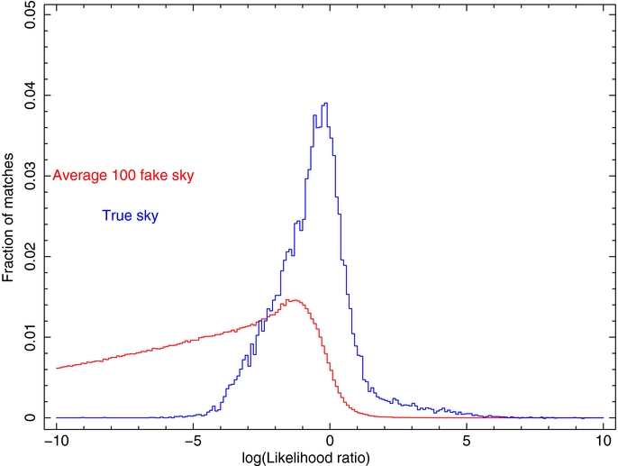
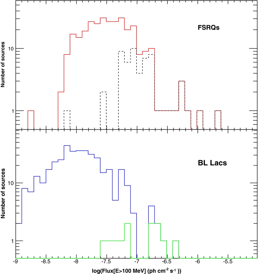
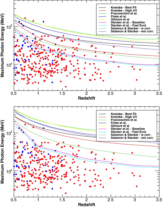