Unified single-cell analysis of testis gene regulation and pathology in five mouse strains
- Washington University School of Medicine, United States
- University of Oxford, United Kingdom
- Oregon Health & Science University, United States
Figures
Figure 1 with 5 supplements
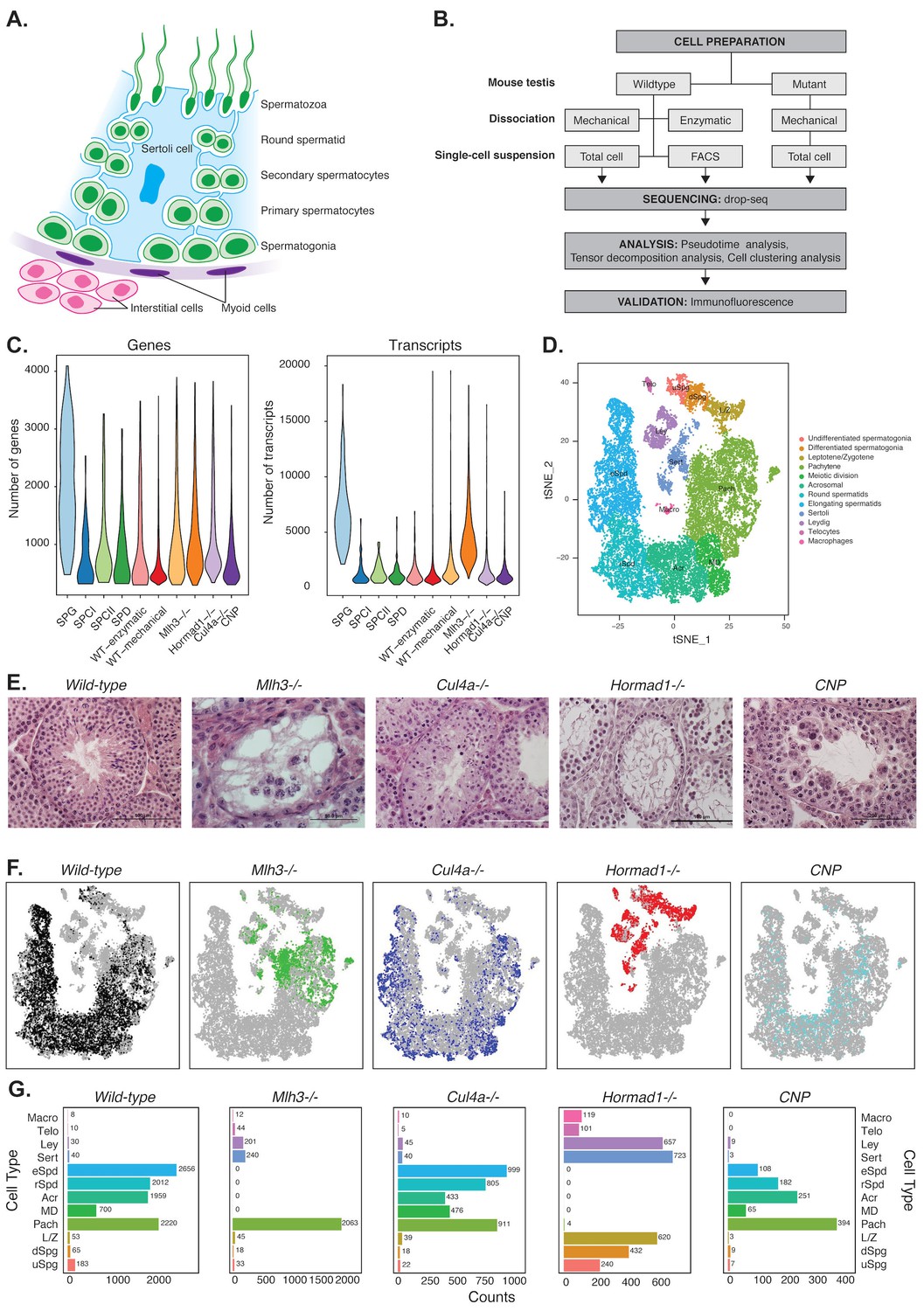
Mapping cellular diversity in the adult testis using single-cell expression profiling.
(A) Anatomy of the testis. Adult testis are comprised of germ cells (spermatogonia, primary spermatocytes, secondary spermatocytes, spermatids and spermatozoa) and somatic cells. Within the seminiferous tubules, there is a population of somatic cells (Sertoli). The tubules are wrapped by muscle-like ‘myoid’ cells. Outside the tubules are a heterogeneous, poorly defined population of ‘interstitial’ somatic cells including Leydig cells and telocytes. (B) Overview of the experiments. To establish the utility of single-cell profiling for testis phenotyping, we performed a series of experiments (i) comparing the quality of traditional enzymatic dissociation and more rapid mechanical dissociation, (ii) comparing the expression profiles of cells from total testis dissociation to testicular cells of known identity purified by FACS, (iii) comparing expression profiles of wild-type animals to cells isolated from four mutant strains with testis phenotypes (Figure 1—figure supplement 1). (C) We used Drop-seq to profile 26,200 cells from wild-type animals and 31,400 cells from mutant animals, with an average of 1155 transcripts/cell and 725 genes/cell (wild-type) and 2223 transcripts/cell and 1133 genes/cell (mutants). (D) We applied SDA and used t-SNE to visualize cells colored by k-means clustering of 20,322 cells, derived from our full dataset of wild-type and mutant animals, into 32 clusters (Materials and methods, Figure 1—figure supplements 1–5). Label assignment clearly indicates a spatial organization of testis cells in t-SNE space, with somatic cell populations flanking the germ cells in small pockets. The full set of 32 clusters has been simplified into 12 major classes for ease of interpretation; the full clustering is shown in Figure 1—figure supplement 2. (E) Histology sections from wild-type and mutant testis, illustrating the phenotypes observed in wild-type and the four mutant strains characterized by Drop-seq. Three of the strains, Mlh3-/-, Hormad1-/- and Cul4-/- have known pathology, while strain CNP represents an unpublished transgenic line with spontaneous male infertility. (F) Mapping of cells from each mouse strain into t-SNE space (colored points) compared to the background of all other strains (gray points). Mutant strains occupy distinct locations within t-SNE space, reflecting the absence of certain cell types in some strains (e.g. Mlh3-/- and Hormad1-/-), and alteration of expression in remaining cells (e.g. Hormad1-/-). (G) Counting individual cell types provides a quantitative phenotype of cellular heterogeneity in each strain.
Figure 1—figure supplement 1
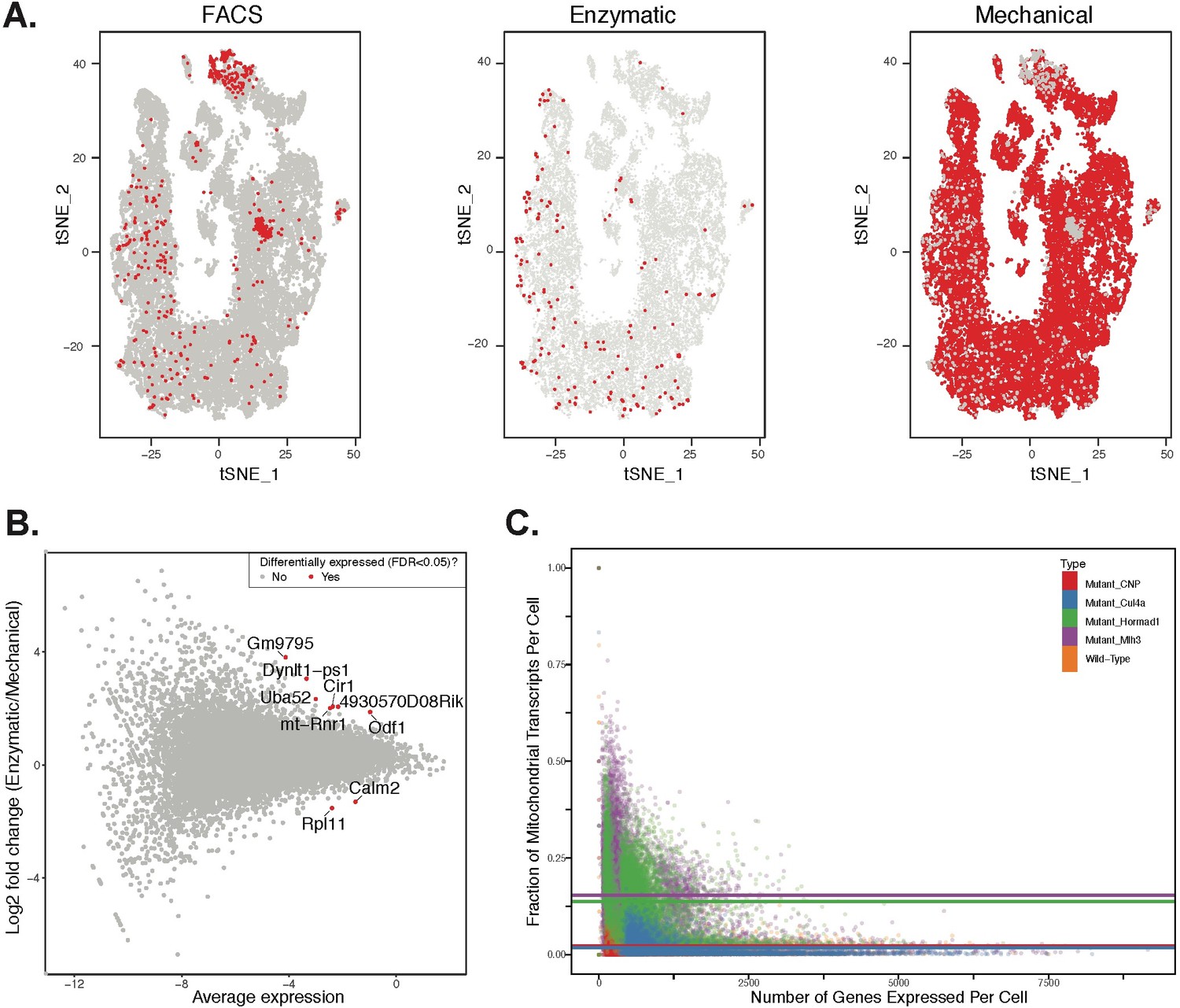
Comparison of effects of dissociation protocols and mutation status on cell ascertainment and single-cell gene expression.
We compared the effects of enzymatic dissociation (SPG, WT1, WT2) and mechanical dissociation protocols (all other batches) on both the ascertainment of cell types (by visualization in t-SNE space) and on single gene expression levels. (A) No obvious batch effects were detected when comparing the t-SNE clustering location of cells isolated by FACS, or either of the two total testis dissociation protocols. (B) We performed differential expression analysis to compare the two dissociation protocols, using all available WT datasets. We compared single gene expression levels for all genes detected by both protocols, summarized here as an M + A plot. The expression profiles from enzymatic and mechanical dissociation showed excellent concordance (R = 0.95). Genes that were detected as differentially expressed by edgeR are plotted in red. (C) When compared to wild-type, cells from mutant strains exhibit significantly higher fractions of transcripts derived from mitochondrial genes, indicative of elevated rates of apoptosis.
Figure 1—figure supplement 2
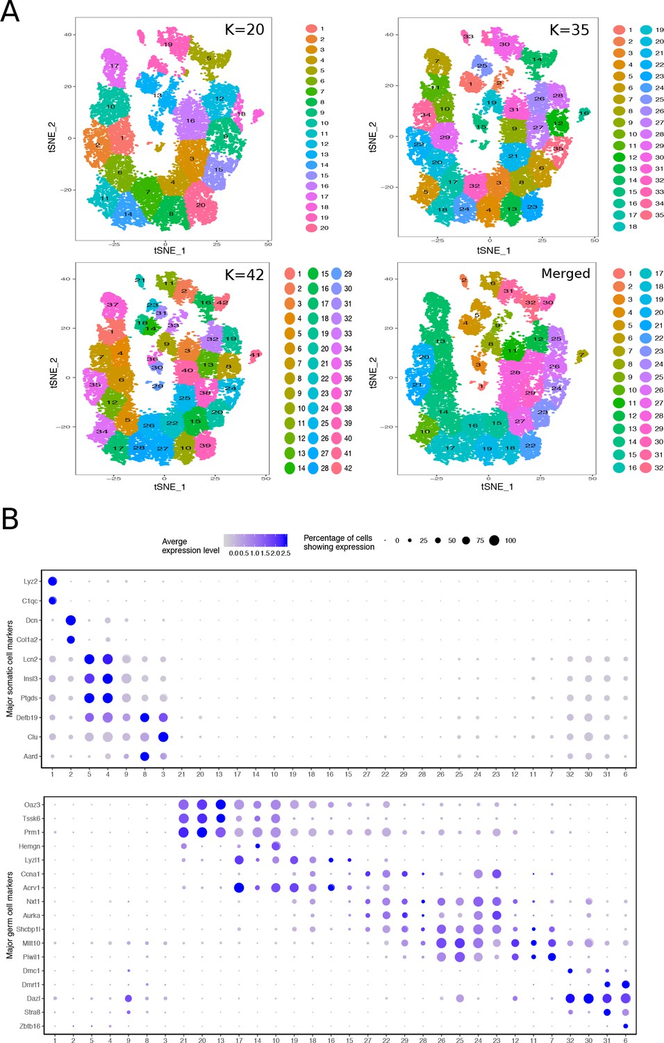
Mapping the Cellular Diversity of the Testis.
(A) We performed k-means clustering analysis of total joint wild-type and mutant cells with several levels of ‘k’ to determine the appropriate level of clustering for cell type identification. Clusters with similar expression profiles were merged using out-of-bag-error (OOBE) method implemented in Seurat, ultimately leading to a final analysis with 32 clusters. (B) Expression of known somatic and germ cell--type specific markers in total joint wild-type and mutant cell clusters.
Figure 1—figure supplement 3
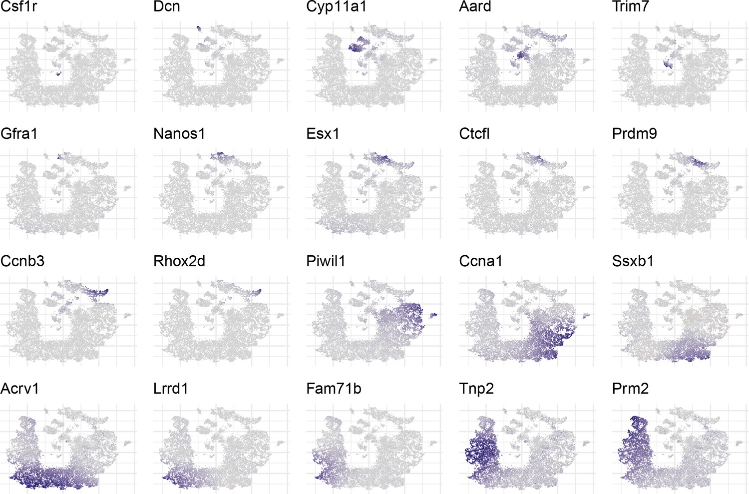
Overview of expression patterns for some well known testis cell markers in t-SNE space.
https://doi.org/10.7554/eLife.43966.005
Figure 1—figure supplement 4
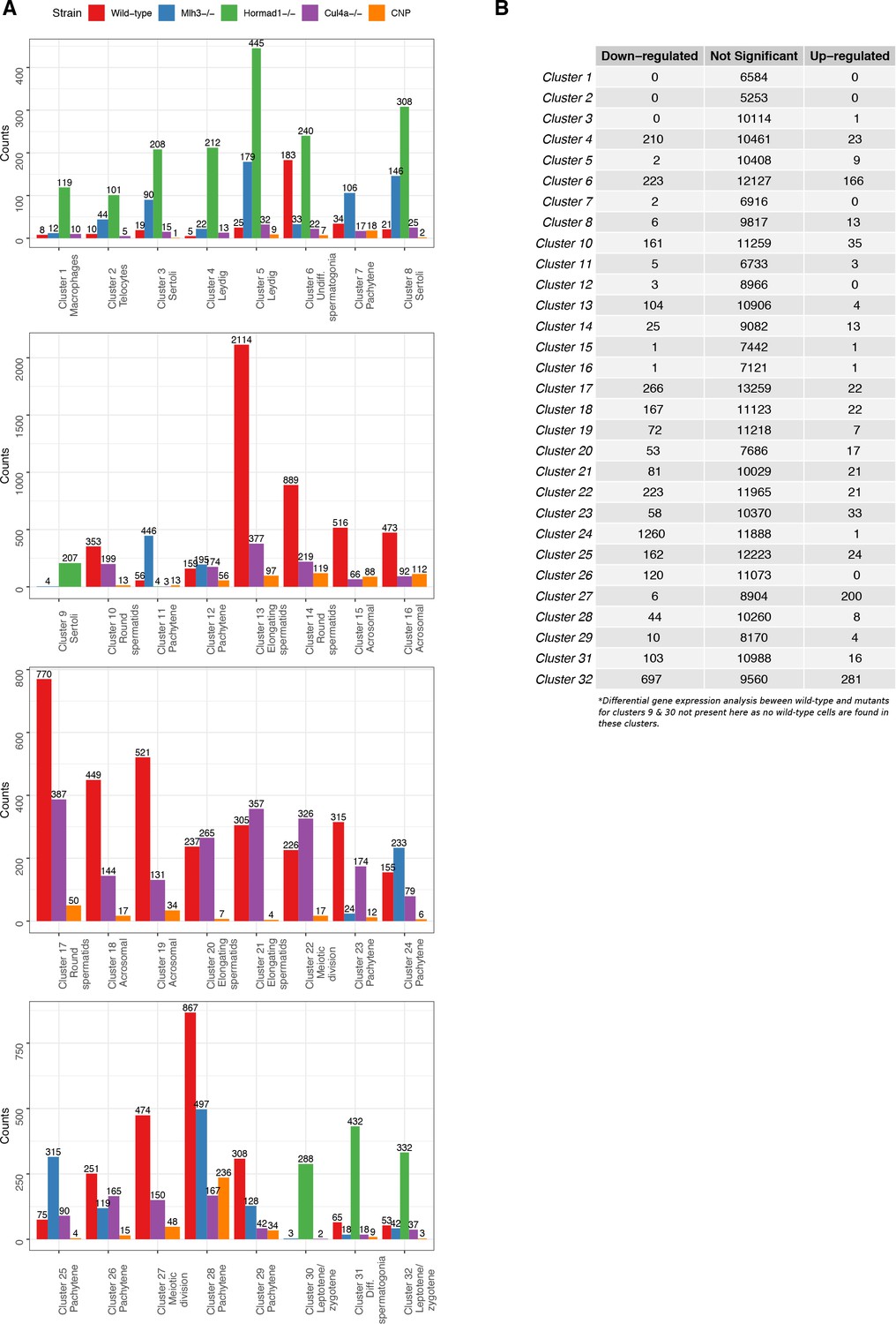
Tabulation of cluster counts by mouse strain and differential expression analysis within clusters.
(A) Count distribution of cells from each mouse strain for 32 clusters in Figure 1—figure supplement 2A (‘Merged’). (B) To explore any clustering bias between wild-type and mutant cells, we performed differential gene expression analysis using edgeR for each cluster between wild-type and mutant cells. Genes that did not express at least five transcripts were filtered. The cut-offs for significant differentially expressed genes were log-fold change of 1 and false discovery rate (FDR) adjusted p-value<0.05.
Figure 1—figure supplement 5
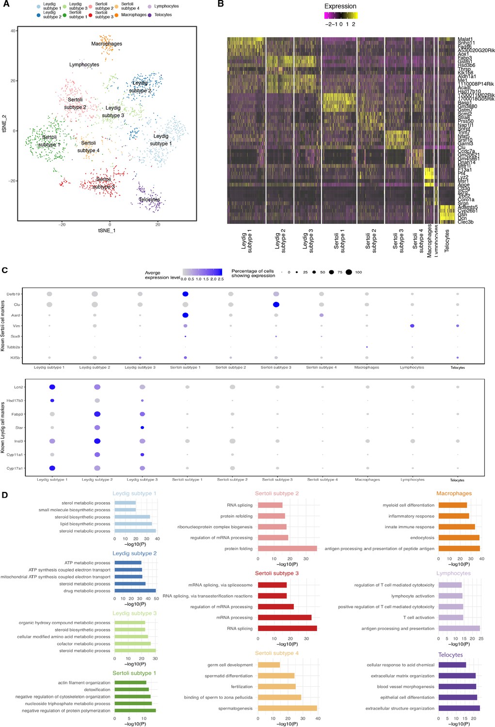
Dissection of Somatic Cell Population Heterogeneity.
(A) Visualization of somatic clusters on t-SNE. We extracted somatic cell clusters (clusters 1, 2, 3, 4, 5, 8 and nine from Figure 1—figure supplement 2A (‘Merged’) and performed additional k-means clustering analysis. Clustering analysis identified 4 Sertoli cell subtypes, 3 Leydig cell subtypes, one macrophage population, one lymphocyte population and one telocyte cell population. (B) Then we performed differential expression analysis using Seurat’s built-in function ‘FindAllMarkers()’ between different somatic cell clusters to identify differentially expressed genes and visualization of top five differentially expressed genes is shown in the heatmap. (C) Expression of known Sertoli and Leydig cell markers across all somatic cell clusters. (D) We performed gene ontology (GO) enrichment analysis on the lists of differentially expressed genes identified for each somatic cluster. P-values are adjusted with Benjamini-Hochberg method.
Figure 2
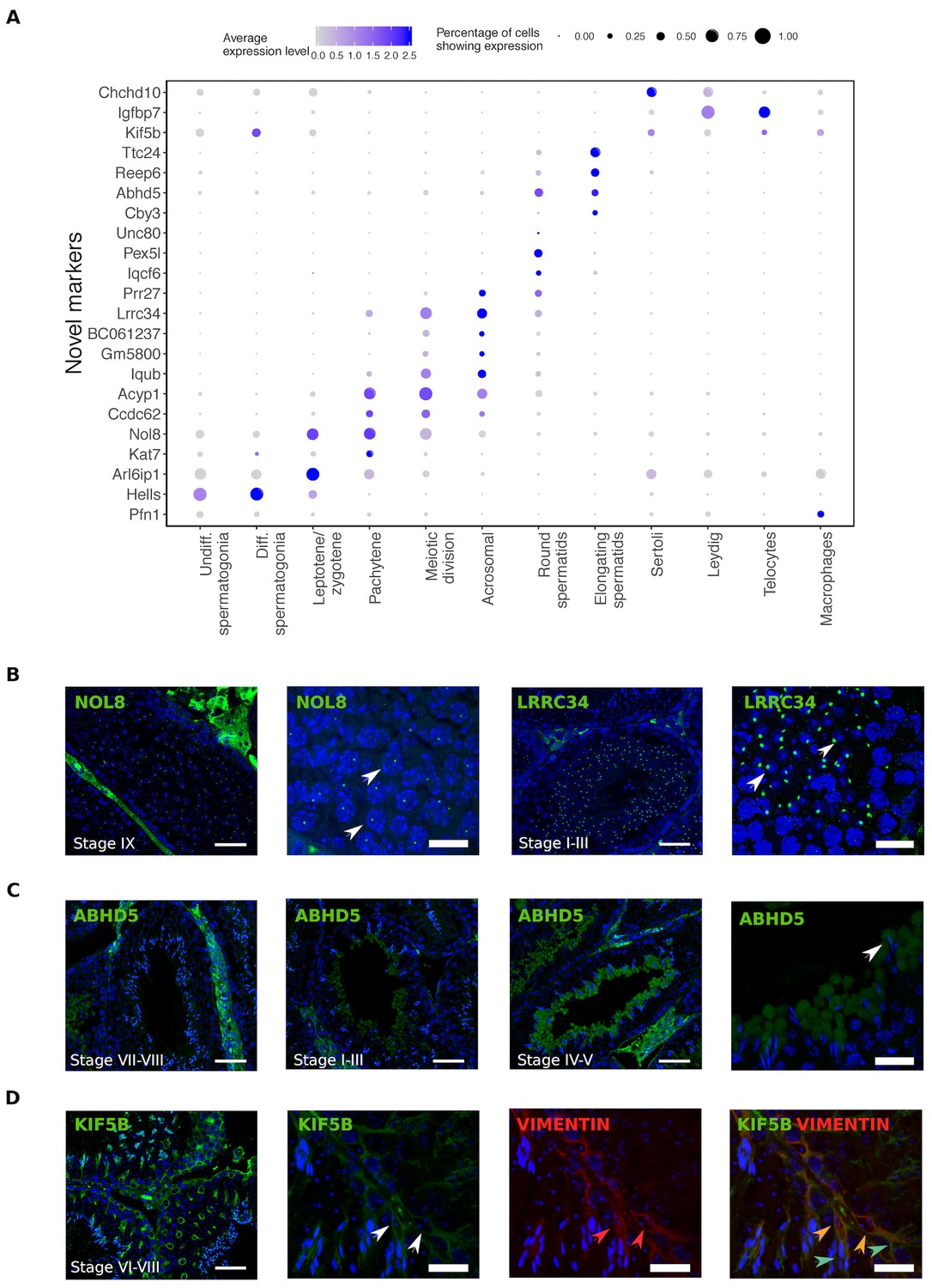
Identification of novel cellular markers from single-cell data.
(A) Across major cell-type clusters, we identified 22 gene expression markers specific to one cell type or aspect of spermatogenesis and not previously reported. Here we show the expression levels of these genes. Expected protein expression patterns for Nol8, Lrrc34, Abhd5, and Kif5b were confirmed, but the antibodies for Acyp1, Ccdc62, and Unc80 did not show positive staining in any testicular cell types,which could be an antibody-related problem or an indication that these RNAs were not translated. (B–D) Thin scale bar, 50 µm; thick scale bar, 20 µm. (B) Nol8, a nucleolar protein, marks primary spermatocytes while Lrrc34 marks nucleoli in round spermatids (white arrowheads) (C) Within the tubules, Abhd5 marks specific cytoplasmic regions of elongating spermatids destined to form the residual body (white arrow head) and staining intensity peaks during seminiferous tubule stages IV-V. (D) Kif5b marks Sertoli cells within seminiferous tubules (white arrow head). We co-stained Kif5b with a well-known Sertoli cell marker, Vimentin (red arrow head), and indeed both proteins colocalize to Sertoli cells (orange arrow head). Co-staining also reveals that Kif5b staining extends further out in the cell body (blue-green arrow head) than Vimentin.
Figure 3 with 5 supplements
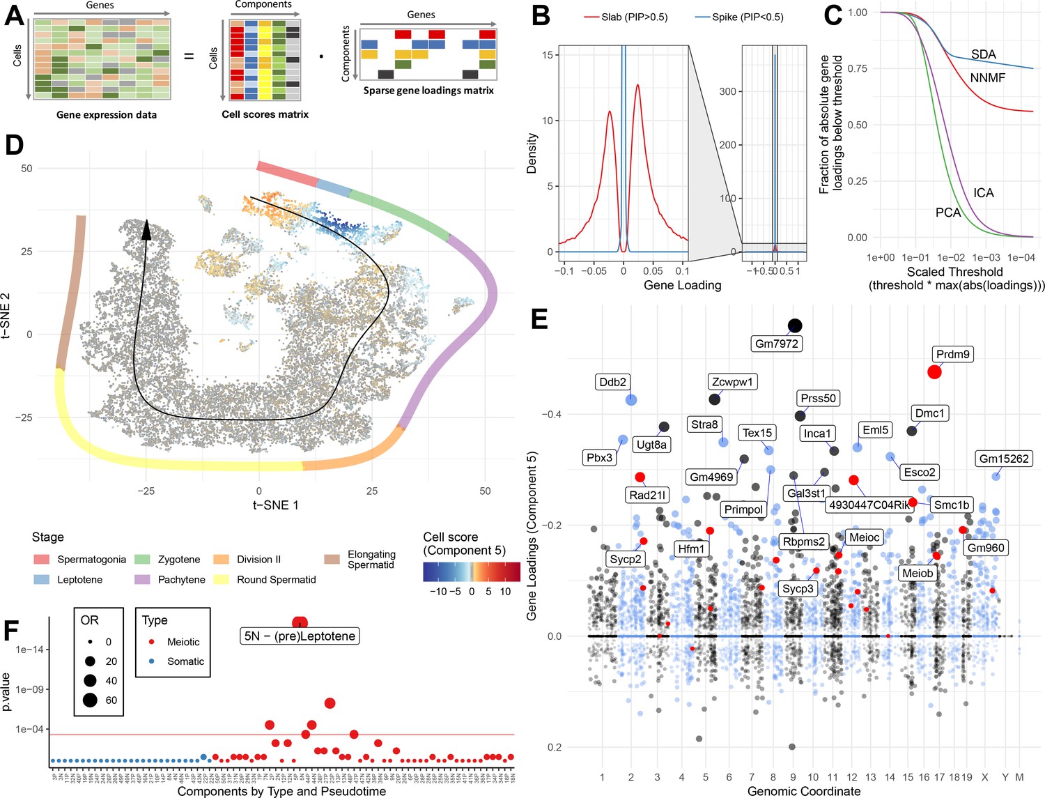
SDA identifies gene modules and maps them to cells.
(A) We applied sparse decomposition analysis (SDA) to identify latent factors (‘components’) representing gene modules. These components are defined by two vectors – one that indicates the loading of each cell on the component, and one that indicates the loading of each gene on the component. (B), SDA uses a spike and slab prior on the gene loadings to induce sparsity (a point mass at 0 and a centered normal distribution respectively). PIP = Posterior Inclusion Probability that a gene loading is not equal to zero (i.e. not in the spike). The figure shows the density of gene loadings over all components with loadings separated into genes with PIPs > 0.5 (20%) versus <0.5, indicating the sparsity of resulting gene loadings. (C) SDA produces sparser representation of gene loadings compared to other matrix factorizations: NNMF, ICA and PCA. For each method, the fraction of all absolute gene loadings exceeding a ‘no loading’ sparsity threshold is shown, normalized by the maximum absolute loading across all components for that method. (D) We fitted 50 SDA components using 20,322 wild-type and KO cells (see also Figure 3—figure supplements 1–5). We illustrate component 5. The loadings of component 5 in t-SNE space highlight a cluster of cells at the leptotene early meiotic developmental stage. Black arrow: the principle curve fit to the germ cell data, corresponding to the developmental ordering of each cell progressing through spermatogenesis. The colored segmented line shows broad staging of spermatogenesis. (E) Genomic location versus loadings for component 5. Most genes have near-zero loadings, but a fraction have non-zero loadings, including the well-known histone methyltransferase Prdm9. Red genes: GWAS hits for human recombination rate. (F) Component 5 is highly and specifically enriched for GWAS hits of human recombination rate. OR: Odds Ratio. P value by FET (main text). Positive (P) and negative (N) loadings are tested separately. For one-sided components (cell score range ratio >5) the minor side is omitted. Red horizontal line: p=0.05 after Bonferroni correction for multiple testing.
Figure 3—figure supplement 1

Overview of cell score loadings in t-SNE space for all components produced by SDA except single cell components (1, 4, 8, 14, and 46).
The component number and biological interpretation of the component are labeled above each panel.
Figure 3—figure supplement 2
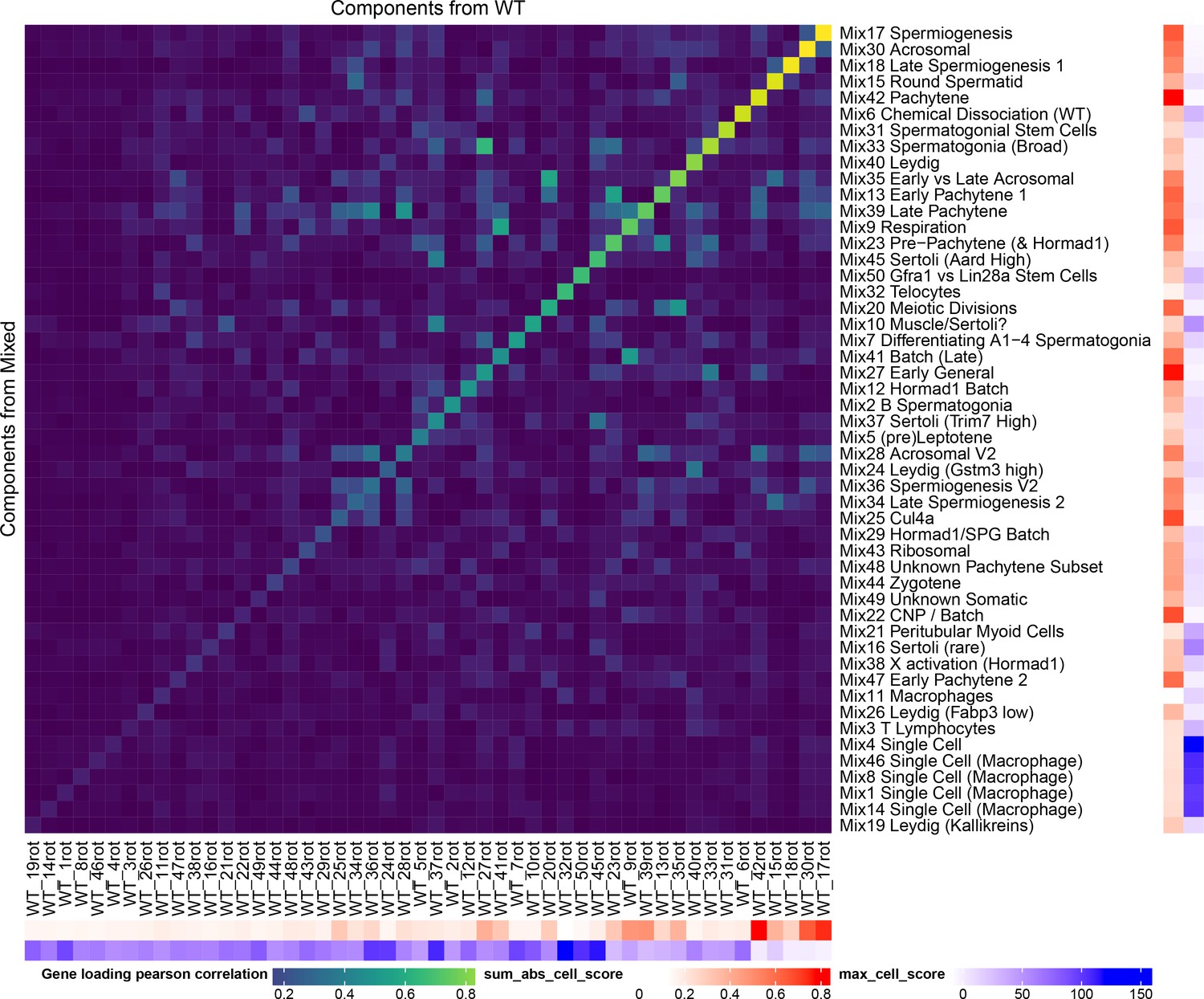
Robustness of SDA Results.
All of the SDA results presented in the main text are derived from a combined analysis of all wild-type and mutant cells (the ‘Mixed’ analysis). In order to quantify the robustness of our conclusions to this decision to combine mutant and wild-type strains, we performed a separate SDA analysis using just wild-type cells (the ‘WT’ analysis). Here we show as a heatmap the pearson correlation of component gene loadings between a procrustean rotation of the WT gene loadings and the Mixed SDA gene loadings. The ‘sum abs cell score’ annotation shows the sum of the absolute cell scores for that component (larger number indicates a more important component). The ‘max cell score’ annotation indicates the maximum cell score for each component (a larger maximum indicates overfitting to a single/small number of cells). The most important WT components have high correlations with components in the mixed SDA run. Some components such as Mix38 X activation do not appear in the WT decomposition because they represent mutant-specific processes. Other components such as Mix44 Leptotene-Zygotene do not appear as these cells are enriched in mutant samples due to the lack of later cells.
Figure 3—figure supplement 3
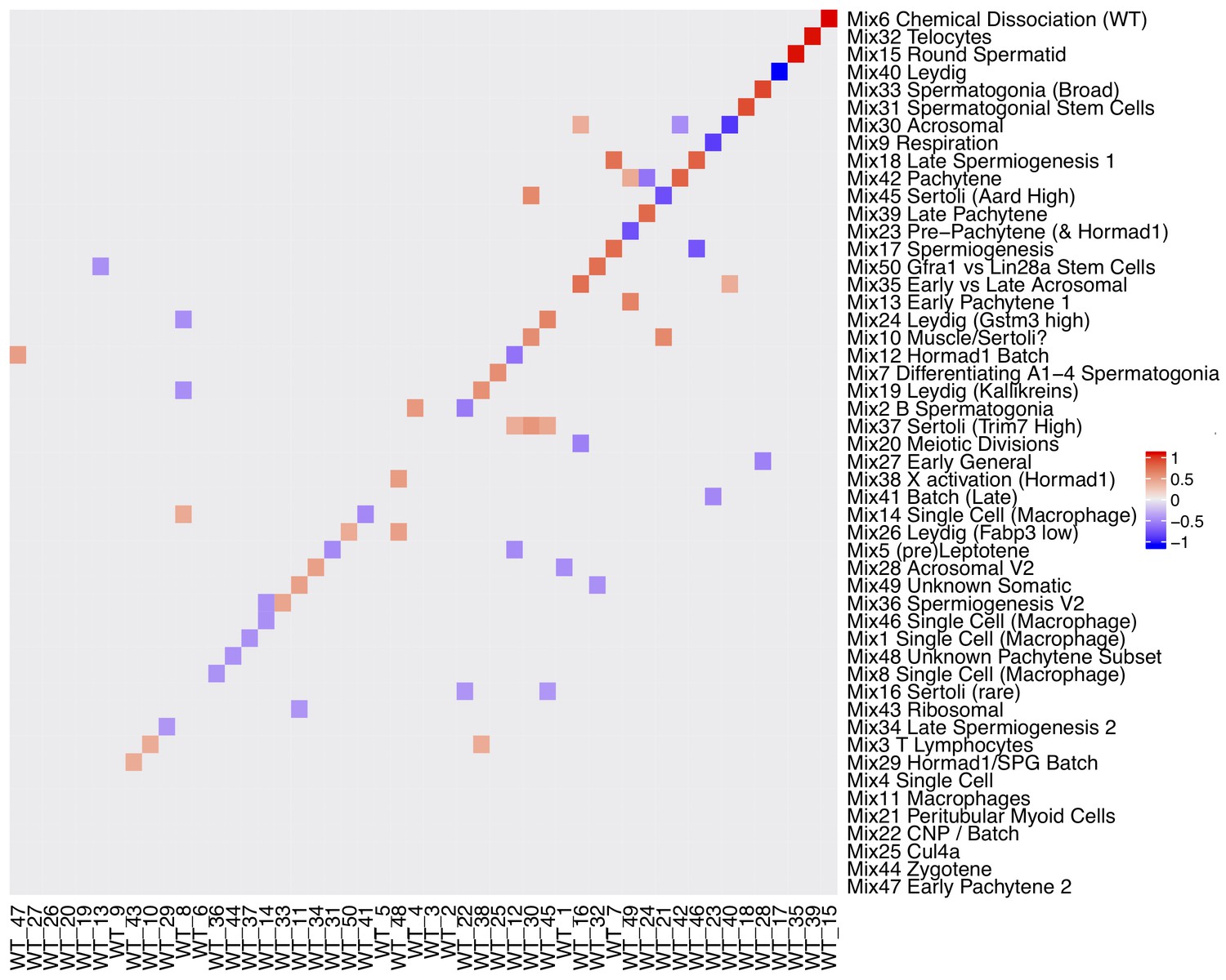
Rotation Matrix.
Factor analyses naturally have a degree of unidentifiability, whereas in SDA the sparsity prior helps to make the model identifiable across different seeds for different data the gene loadings matrix may be a rotated version in which components are linearly split or combined. A procrustean rotation can align two matrices (here gene loadings) onto an equivalent set of axes. This heatmap shows the procrustean rotation matrix (with absolute values < 0.35 rounded down to 0). For example Mix component 17 spermiogenesis is a linear combination of WT component 46 and 7.
Figure 3—figure supplement 4
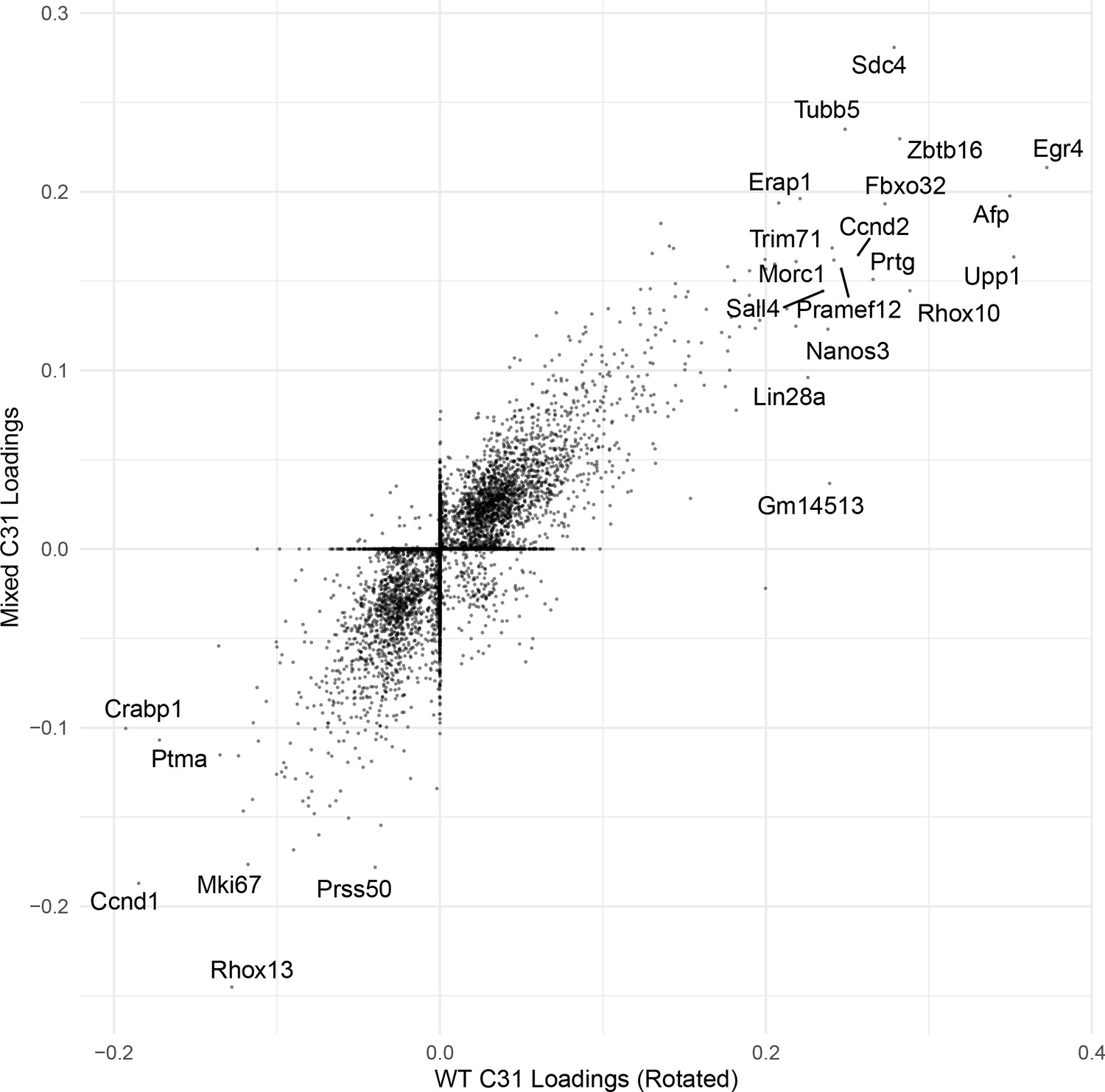
Correlation of C31 gene loadings.
An example scatterplot comparing the gene loadings for one cognate SDA component (C31) between WT and Mixed SDA runs. The correlation is high.
Figure 3—figure supplement 5
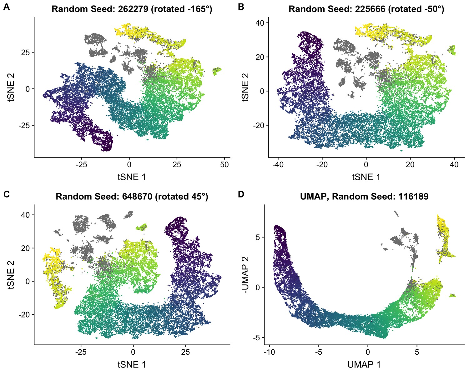
Robustness of t-SNE embedding.
(A–C) To quantify our uncertainty in the t-SNE embedding, we performed multiple t-SNE analyses with random seeds were used. The cells are colored by the pseudotime used in the main text. Somatic cells are colored gray. t-SNE coordinates are rotated about the origin to aid visualization. (D) We also performed dimensionality reduction using UMAP and confirmed that it gave a pseudotime embedding consistent with t-SNE. The cells are colored by the pseudotime used in the main text.
Figure 4 with 4 supplements
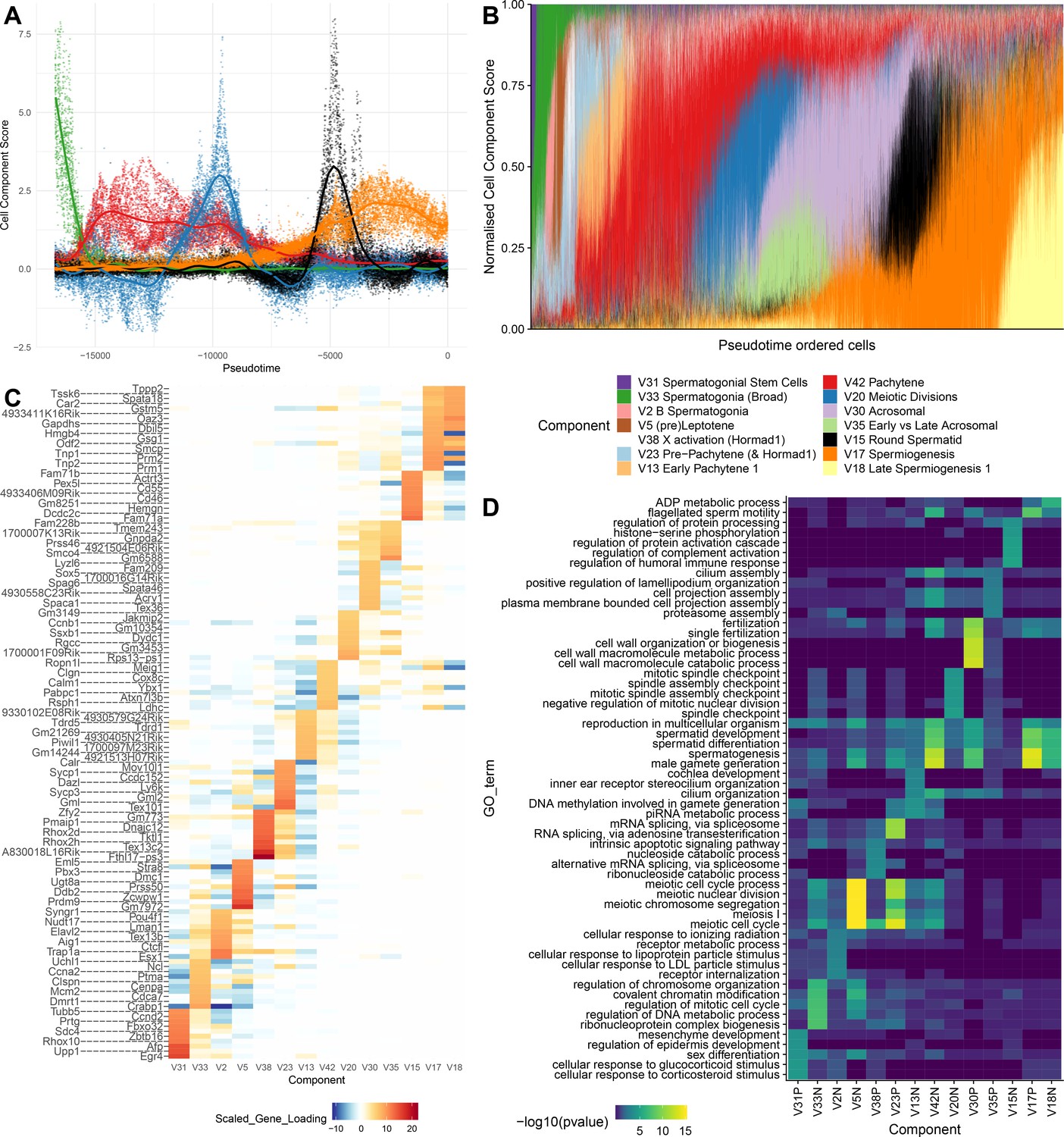
SDA components overlap but represent distinct processes.
(A) For five example components, the cell scores for each cell are plotted through pseudotime, indicating strongly overlapping dynamically varying component activity. Component signs were chosen to be mainly positive (components have arbitrary sign). Color mappings as in panel B. (B) Stacked bar plot of cell component loadings for 14 germ components sorted by cell pseudotime. Each column corresponds to an individual cell and the total positive component loadings for each are normalized to one after flipping components to be mainly positive. Factorization by SDA indicates that transcription during spermatogenesis can be represented as an overlapping series of components in time, coming on and off gradually on different timescales. See also Figure 4—figure supplements 1–2 for alternative visualizations of components in pseudotime. (C) Furthermore, these components are comprised of distinct gene sets driving distinct biological processes. Shown are the top 10 gene loadings for each of the components in (B) represented as a heatmap. Most genes have strong loading on only one component. (D) Likewise, a gene ontology enrichment analysis for biological processes in the top 250 genes for each component indicates largely non-overlapping enrichments across components. More in-depth analysis of GO enrichments and gene loadings for each component allow separation of components into biological and technical effects (Figure 4—figure supplements 3–4).
Figure 4—figure supplement 1
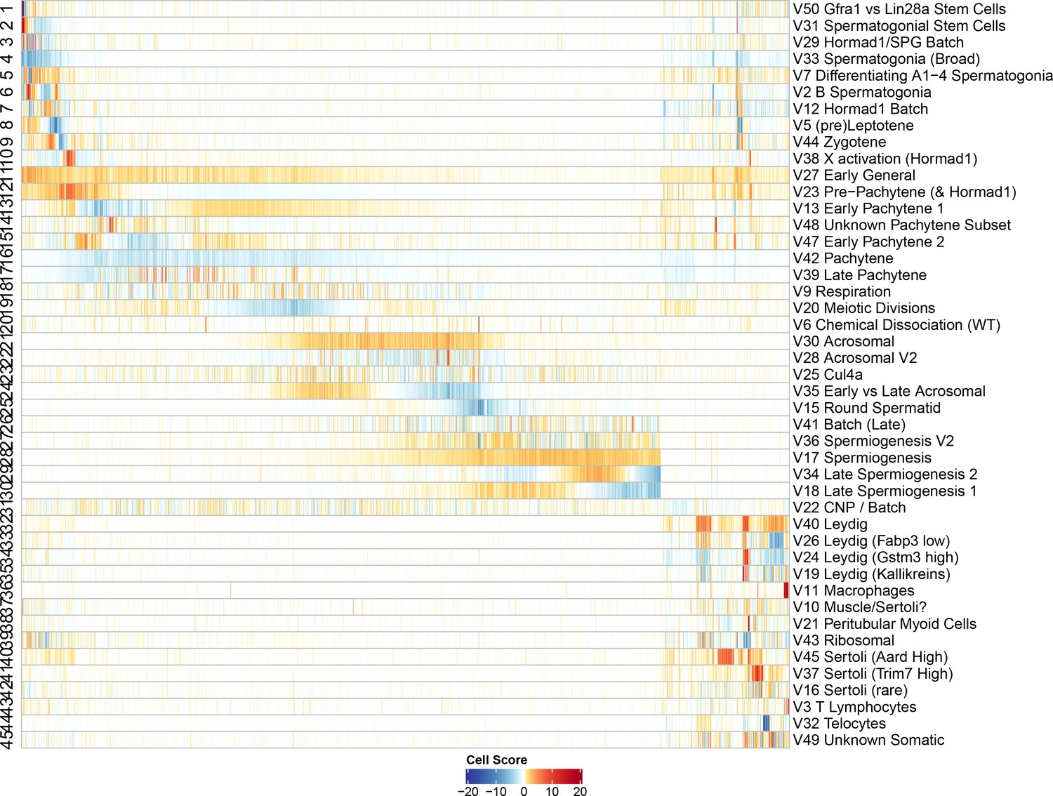
Heatmap of SDA component scores.
Cell scores for all SDA components except single cell components. Each column corresponds to an individual cell and each row is a component. The columns and rows are both ordered by pseudotime, except for the somatic cells/components in which the components are ordered alphabetically and cells are ordered by cluster label assigned by hierarchical clustering applied to all cells (method ward.D2, k = 25). Absolute cell scores greater than 20 have been rounded down for plotting.
Figure 4—figure supplement 2
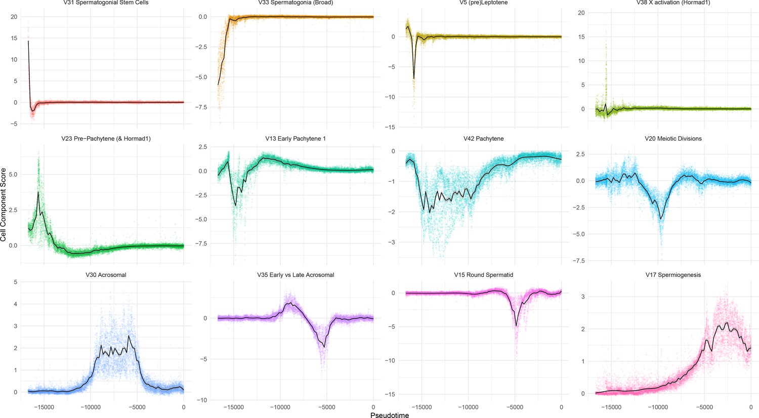
Overview of Individual SDA Components.
Cell scores plotted as a function of pseudotime, for 12 representative SDA components.
Figure 4—figure supplement 3
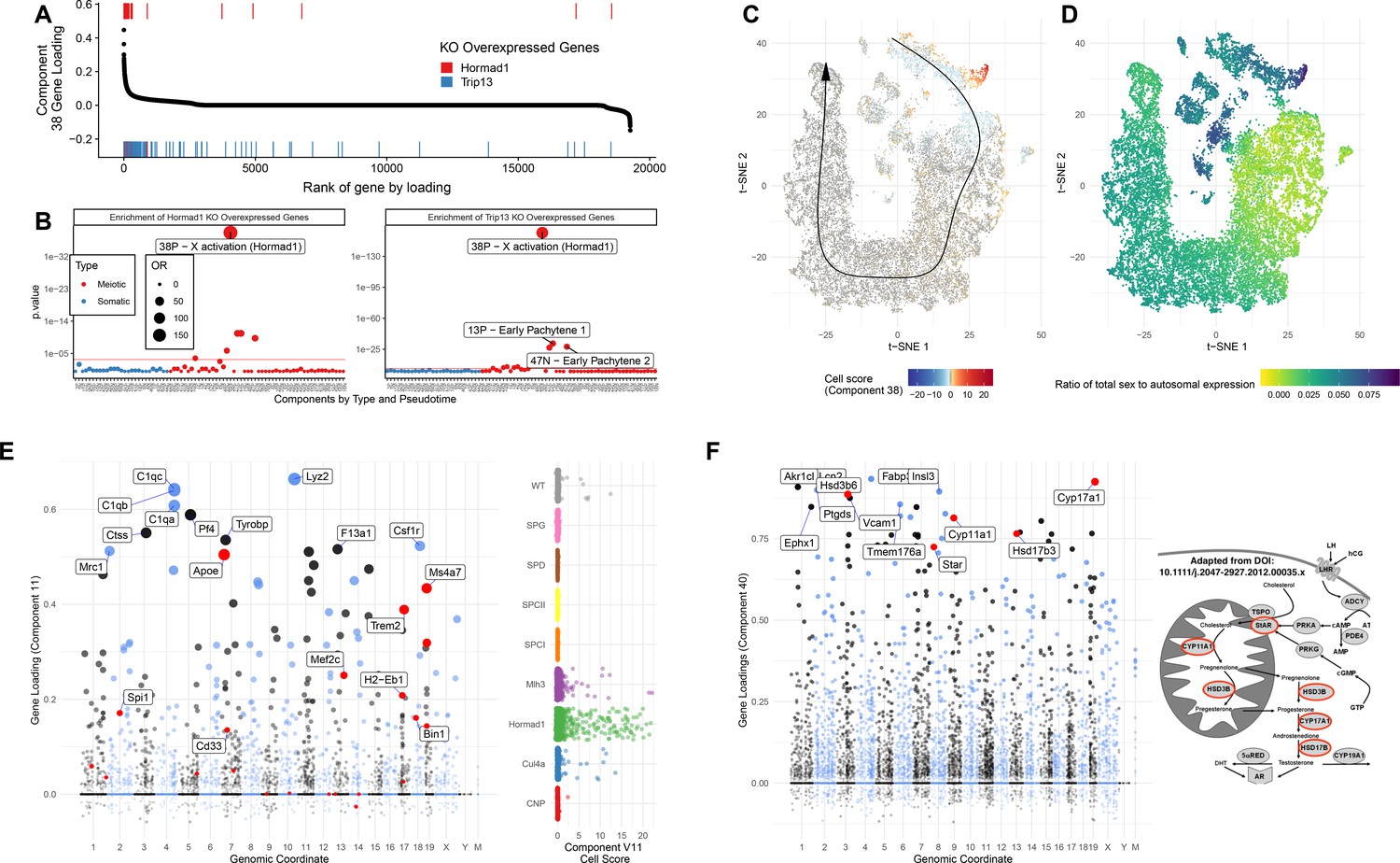
Detailed Analysis of Individual SDA Components.
(A) Comparison of genes overexpressed in Hormad1-/- DropSeq and genes IDs previously identified as overexpressed in both Trip13-/- and Hormad1-/- mutants. Component 38 (X Activation) gene loadings are shown ordered by rank (high-to-low) with the genes previously identified as overexpressed in Hormad1-/- and Trip13-/- mice highlighted as rug plots. (B) Fisher’s test was used to test for enrichment of genes previously identified as overexpressed in Hormad1-/- and Trip13-/- mice in the top 500 genes of each component. Positive and negative loadings for each component are analyzed separately; thus 38N is the negative gene loadings for component 38 and 38P the positive ones. The positive loadings of component 38 are highly and specifically enriched for these genes. Component enrichments are further colored red and blue to indicate the primary cell type with loading on each component (red = germ cell, blue = somatic cell). (C) Cell scores for component 38 in t-SNE space. The cells with component 38 active are localized to a group of cells which diverge from the pseudotime-line just before pachytene. (D) MSCI in t-SNE space. The cells with active component 38 also have a high ratio of sex to autosome expression ratio, showing that not only do these cells fail to silence sex linked genes but they are actively overexpressed. (E) Gene loadings and cell scores for component 11 (Macrophages). Genes with GWAS signals for Alzheimers disease are highlighted in red. (F) Gene loadings for component 40 (Leydig cells), with key genes of testosterone synthesis highlighted in red. The pathway of testosterone synthesis is shown with genes that have high loadings in component 40 highlighted (Adapted from Stojkov et al., 2013).
Figure 4—figure supplement 4

Components representing batch effects and cellular respiration.
(A and B) Gene loadings and cell scores for component 22. Experimental batches with lowest cell scores were all sequenced on MiSeq rather than HiSeq and many of the genes with the highest loadings are ribosomal proteins suggesting this is a technical batch effect component of sequencing platform. (C and D) Example cell and gene loadings for a likely batch effect driven by the use of different individual mice. Note that for the first 2 Hormad1-/- libraries, generated from a mouse of 4 months old, the cell loadings are positive, while for the last library, generated from a mouse 4 months and 3 days old, the cell loadings are negative. (E) Gene loadings for component 9. Genes that are (non-assembly) components of the electron transport chain proton pump genes are highlighted in red. This gene set is defined by the genes that match the regex ‘Uqc|Cox|Ndu’. Pseudogenes, and genes with ‘assembly|like’ in their name were excluded.(F) Enrichment of genes that are (non-assembly) components of the electron transport chain proton pump genes in the top 500 genes from each component.
Figure 5 with 1 supplement
Evaluation of imputation using the SDA model.
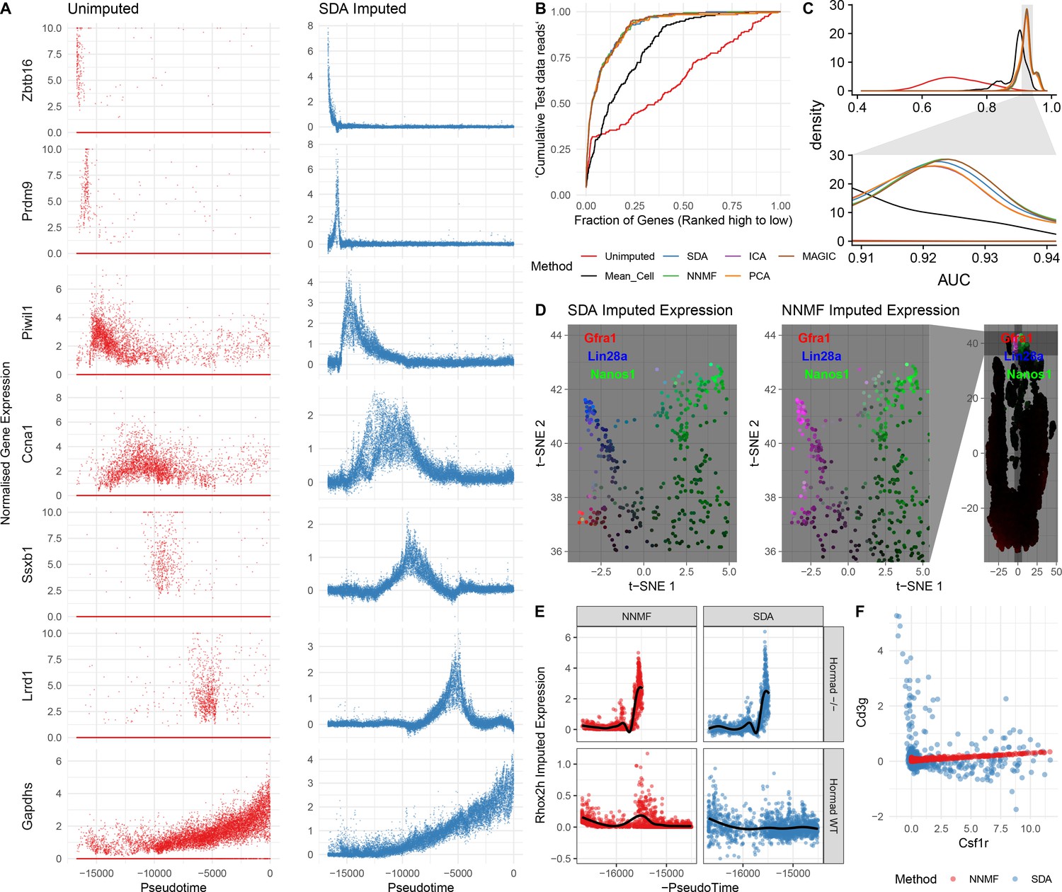
(A) Here, we illustrate the ability of SDA-based imputation (Materials and methods) of gene expression values in single cells to improve the signal/noise ratio of expression, for seven genes with strong developmental regulation. Note in the imputed expression ‘dropouts’ at 0 are recovered and there is less outlying expression. (B) To test the utility of SDA-based imputation, we created separate training/test data (Materials and methods). From the training data we constructed seven predictors of gene expression in the test data for each cell (‘Unimputed’ using the training data directly, ‘Mean Cell’ using the mean across all cells, matrix factorisation approaches SDA, PCA, ICA, NNMF, and a dedicated imputation approach, MAGIC). We compared the ability of each predictor to rank the gene expression in the test data for each cell, quantified as the area under the Rank Prediction Accuracy Curve (RPAC). Shown is an example RPAC for these predictors when applied to the test data for a single cell. (C) Comparison of AUCs (Area under the RPAC curve) for all cells using various methods (same color scheme as part B). (D) SDA produces multiple components for spermatogonia. Shown are zoomed in versions of the t-SNE projection (with full t-SNE for context): cells are colored by expression using a three channel ternary color scheme with the amount of blue, green, red representing the respective expression levels of Lin28a, Nanos1, and Gfra1. By assigning only one component for undifferentiated spermatogonia, NMF predicts Gfra1 and Lin28a are expressed in the same cells resulting in a pink hue (See also Figure 5—figure supplement 1B, no correlation for SDA component 50 Gfra1 Stem Cells). For selection of component see Materials and methods. (E) Imputed expression of X chromosomal gene Rhox2h from either the SDA or NNMF decomposition, split into cells we know to be either WT or Hormad-/- genotype. NNMF predicts a peak in Rhox2h expression even in the WT cells, in which X chromosome activation due to Hormad1 KO does not occur. (F) NNMF does not assign separate components for the innate and adaptive immune cells (See also Figure 5—figure supplement 1B, no correlation for the SDA component 3 Lymphocytes). NNMF does not predict high expression of the adaptive immune cell marker Cd3g (T-cell surface glycoprotein CD3 gamma chain), and when it predicts any expression it increases linearly with the innate immune cell marker Csf1r (Macrophage Colony-Stimulating Factor 1 Receptor, or Cd115). SDA on the other hand correctly predicts that Cd3g and Csf1r are not coexpressed in the same cells.
Figure 5—figure supplement 1
Imputation from SDA and Other Matrix Factorization Methods.
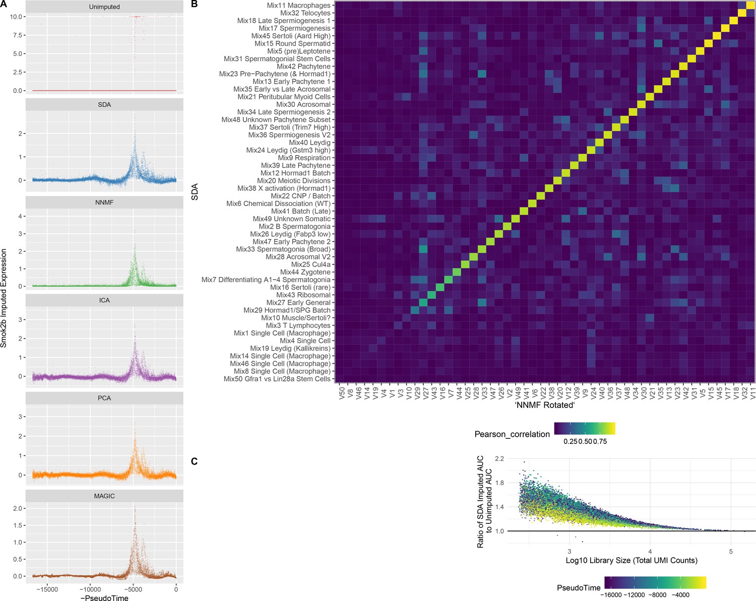
(A) Imputed expression of an example gene (Smok2b) for different methods, to illustrate the similar predictions as shown in Figure 5B and C. (B) Overall, NNMF infers similar components to SDA. The heatmap shows Pearson correlations between different pairs of gene loading vectors from SDA and NNMF (with procrustes rotation applied, Materials and methods). (C) The fold improvement in AUC when comparing SDA imputation to the unimputed data, plotted as a function of cell library size. The gain in accuracy from SDA imputation is inversely correlated with library size that is the cells with low UMI count have most to gain.
Figure 6 with 1 supplement

Insights into sex chromosome biology from SDA.
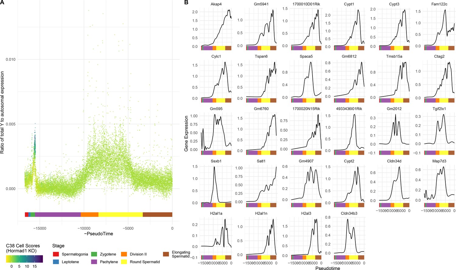
(A) Pseudotime analysis provides quantitative, high-resolution insights into meiotic sex chromosome inactivation (MSCI). The sum of imputed expression for all genes on the X chromosome divided by that of the autosomes (y-axis) drops to almost 0, showing near-complete MSCI before gradually partially recovering. A similar profile is observed for genes on the Y chromosome (Figure 6—figure supplement 1A). (B) We do not observe that haploid cells obviously split into two populations due to lack of sex chromosome transcript sharing, in part A. Here were simulate what we might expect to see if there was indeed a lack of sharing (Materials and methods). (C) No evidence supporting prior report of genes escaping MSCI. Smoothed expression values (unimputed, gam smoothing with formula ‘y ~ s(x, bs = ad)") are shown for each gene reported to escape MSCI (da Cruz et al., 2016) excepting H2al1e, H2al1c, and Gm10096 which were below our dataset’s expression detection threshold. Expression profiles for individual genes are separated in Figure 6—figure supplement 1B. (D) Component 42 (Pachytene) cell scores in t-SNE space. (E) Component 42 gene loadings. This component represents genes active during the pachytene stage of meiosis; note the striking lack of sex chromosome gene loadings, due to MSCI.
Figure 6—figure supplement 1
Single-gene analysis of MSCI.
(A) As for Figure 6A, but Y chromosome instead of X. (B) As for Figure 6C, but each gene is shown individually.
Figure 7 with 2 supplements
Components show shared cis-regulatory features.
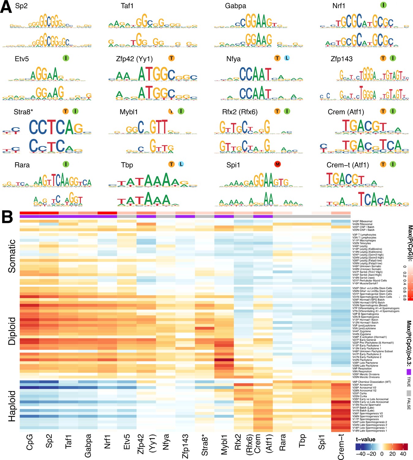
(A) Motifs discovered from the promoter sequences of genes with high component loadings. In each motif logo pair the lower logo shows the de novo inferred motif and the upper logo shows the motif in the HOCOMOCO database best matching the de novo motif. Orange ‘T’ indicates this transcription factor is highest expressed in testis in the GTEx database (half T indicates second highest). Green ‘I’ indicates that a mouse knockout of this gene is infertile. Blue ‘L’ indicates a mouse knockout of this gene is embryonic lethal. Red ‘M’ indicates this gene is required for macrophage development. The notation ‘Crem-t (Atf1)’ indicates that we suspect that the true transcription factor recognizing the motif is not the closest matching database-motif (Atf1). * the (upper) STRA8 motif shown is from Kojima et al., rather than the HOCOMOCO database (B) Association of gene loadings with the probability each de novo identified motif is found in the genes for each component. Coloring is a Z-score from a correlation test between gene loadings and motif probabilities,where red (blue) indicates positive (negative) association. The germ cell components (rows) are ordered by pseudotime. The correlation was calculated for positive and negative parts of the component separately and in the cases where the component is mainly one-sided the other side has been omitted, as have the single cell components. The additional column ‘CpG’ shows the same association test, but with count of promoter CpG dinucleotides, for each component. Across the top of the panel, color bars indicate the maximum probability of there being a CpG at any one position in the denovo motif, and whether that probability is greater than 0.3. See Figure 7—figure supplement 2 for an analogous plot using the HOCOMOCO motif probabilities. We find high and specific enrichment of ChIP-seq targets of STRA8, MYBL1, RFX2 and CREM in the gene loadings of components associated with those motifs, validating our interpretation that covariation of expression of genes within many components reflects shared transcriptional regulation (Figure 7—figure supplement 1).
Figure 7—figure supplement 1
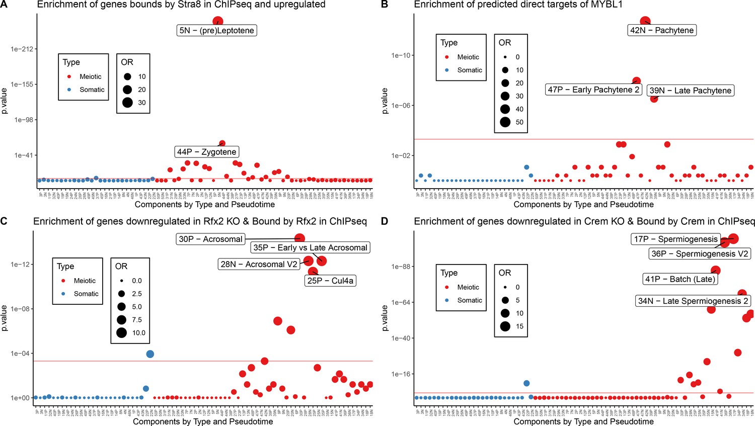
Validation of Motif Inference Using ChIP-seq Data.
As part of the validation that some SDA components represent biological co-expression we tested for enrichment of ChIP-seq defined target genes (Materials and methods) of well-known meiotic transcription factors (A) STRA8, (B) MYBL1, (C) RFX2, and (D) CREM. Enrichment was calculated using Fisher’s test against the top 500 genes in each component (positive and negative loadings separately). OR = Odds Ratio. Red line represents bonferroni corrected p=0.05.
Figure 7—figure supplement 2
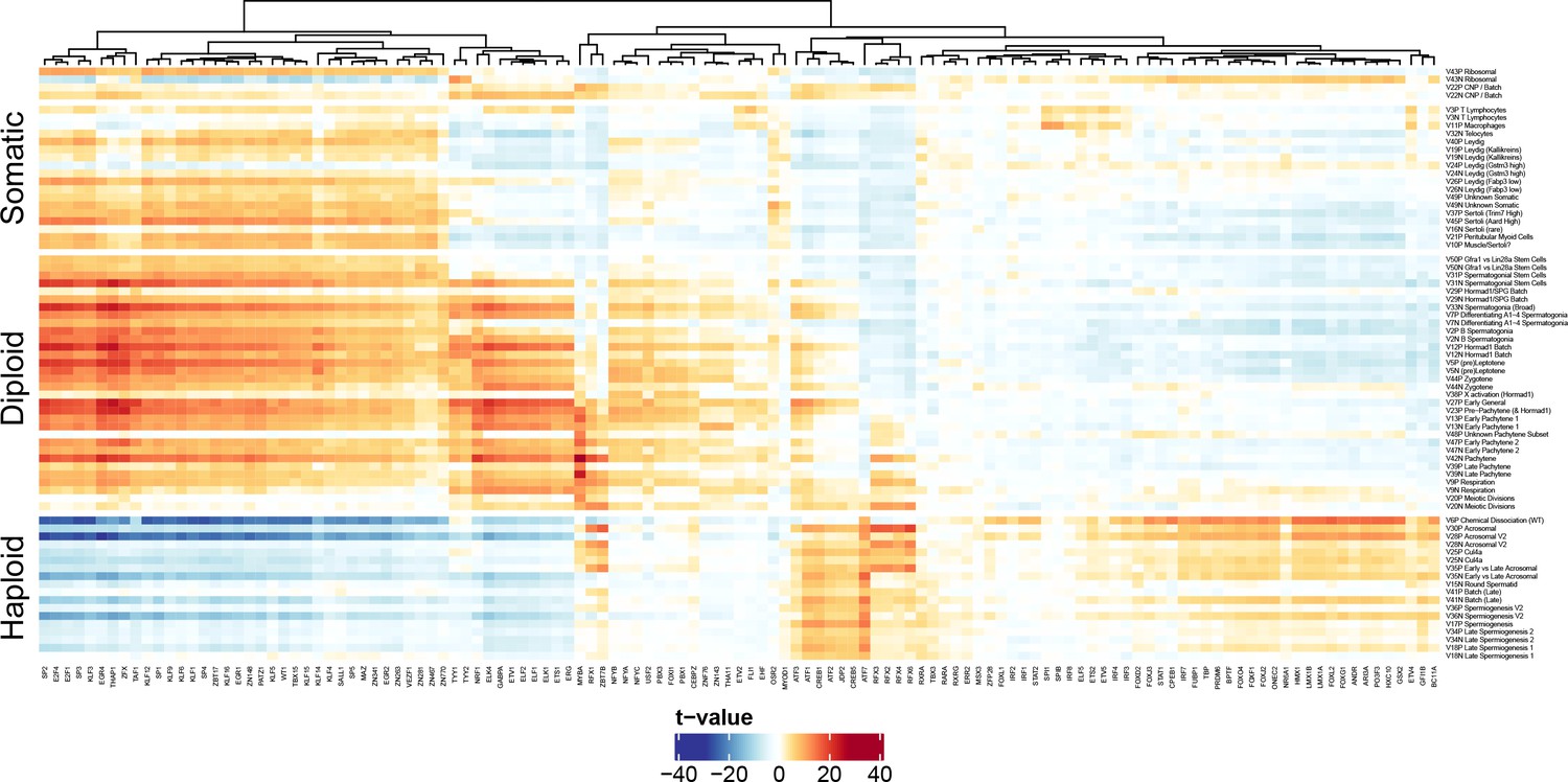
Validation of Motif Inference from SDA Component Loadings.
As described in Figure 7, we performed de novo identification of transcription factor binding sites with enrichment in the cis-regulatory regions of genes loading highly on each SDA component. Here we validate these motifs by quantifying the association of SDA component gene loadings with the probability that each motif is found near the corresponding component genes promoters. The coloring of the heatmap is the test statistic (t-value) from a correlation test between gene loadings and motif probabilities. The t-value follows a t distribution under the null hypothesis of no correlation. Motif probabilities are calculated using the MotifFinder package, and based on the HocoMoco matched motifs. For probabilities based on the de novo motifs see Figure 7 in the main text. The components (rows) are ordered by pseudotime.
Figure 8
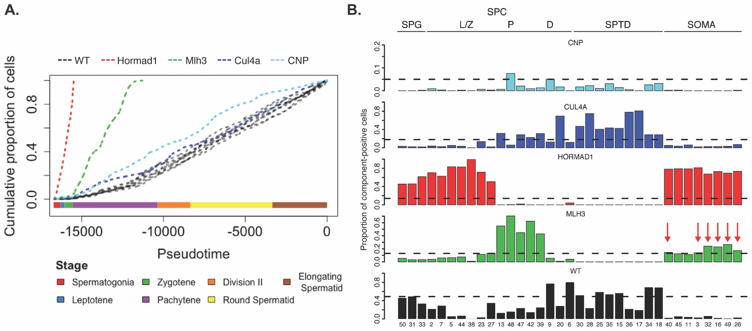
Characterization of mouse mutants with testicular phenotypes using pseudotime and SDA.
(A) The cumulative distribution of cells along pseudotime from each mouse strain. The data clearly indicate that Hormad1-/- cells arrest prior to Mlh3-/- cells in the pachytene stage of spermatogenesis, while Cul4a-/- and CNP mice show quantitative deviation from WT in the abundance of postmeiotic cells. (B) As a way to summarize the SDA analysis of each strain, we plot the proportion of cells with strong component loadings from each strain separately. If cells are randomly distributed across components then we would expect the fraction of cells from each mutant to be the proportion of total cells sequenced from that mutant (dashed horizontal lines). Instead there are clear enrichments of component loadings in particular mutants, providing a fingerprint of pathology for those strains. SDA components are sorted by developmental stage, as indicated by horizontal lines across the top of the panel. SPG = spermatogonial components; L/Z = leptotene/zygotene components; P = pachytene components; D = diplotene components; SPTD = components in spermiogenesis; SOMA = somatic cell components.
Figure 9
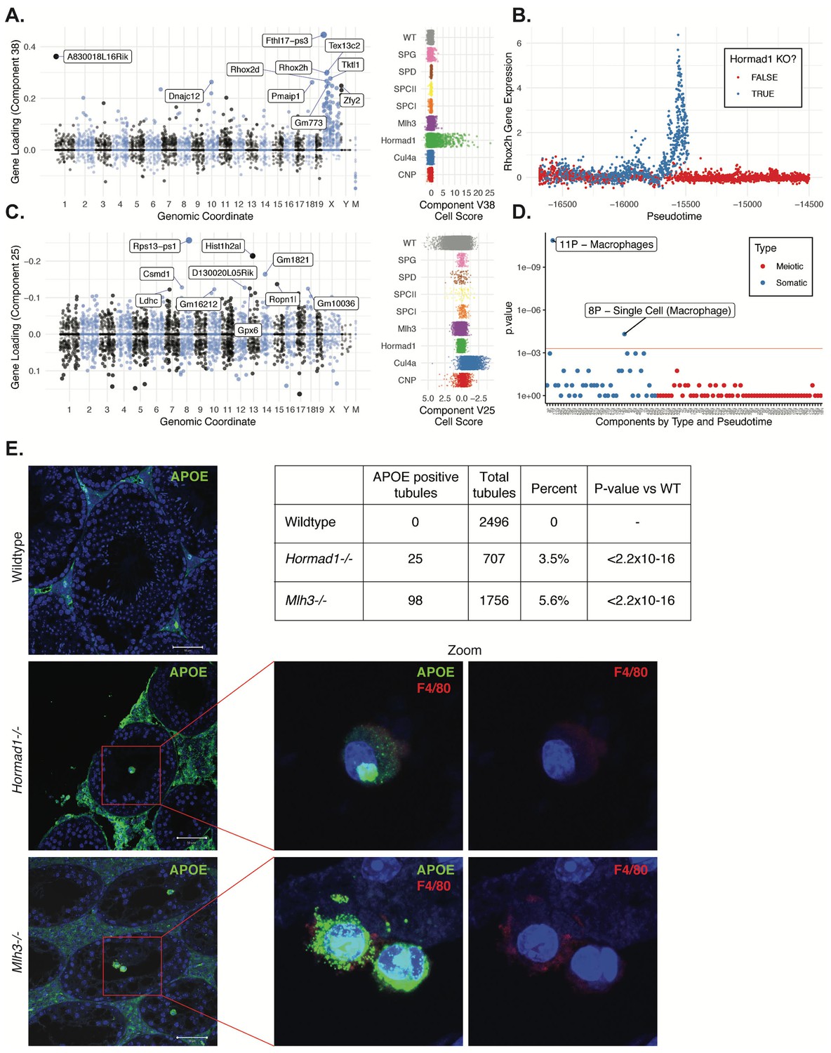
Dissection of strain-specific pathology.
(A) SDA component 38 is comprised largely of genes on the X chromosome, with a gene loading direction that indicates failure of X inactivation. As illustrated by the cell scores (loadings) for this component, it is restricted to Hormad1-/- cells. (B) Pseudotime analysis indicates that Hormad1-/- cells diverge developmentally from all other strains around leptotene/zygotene. In this illustration, the X-linked gene Rhox2h is shown to have low or no expression in all cells prior to meiosis, and then rapidly increased expression specifically in Hormad1-/- cells until this lineage arrests. (C) Component 25 is the component most strongly enriched for Cul4a-/- cells. (D) We identified six components with shared enrichment for both Mlh3-/- and Hormad1-/- cells; these components contained genes with numerous significant GO associations related to Alzheimer’s disease (AD) pathology (main text, Figure 8B). For each SDA component, we tested for association between known AD genes and genes with either positive (P) or negative (N) loadings on that component. AD genes are highly enriched for expression in component 11, corresponding to macrophages. (E) Further investigation of protein expression of AD genes revealed APOE+ (green) cells within the tubules of Mlh3-/- and Hormad1-/- but not WT. These cells showed nuclear morphology different from native germ cells or Sertoli cells, and stain positive for the macrophage marker F4/80. The inset table summarizes raw data on the frequency of APOE+ tubules obtained by microscopy. The frequency of APOE+ tubules is more common in each mutant strain when compared to WT by Fisher’s exact test. Scale bar = 50 µm.
Tables
Key resources table
| Reagent type (species) or resource | Designation | Source or reference | Identifiers | Additional information |
|---|---|---|---|---|
| Genetic reagent (M. musculus) | C57BL/6J | Jackson Laboratory | Cat# 000664 | |
| Genetic reagent (M. musculus) | B6.129-Mlh3tm1Lpkn/J | Jackson Laboratory | Cat# 018845 | Lipkin et al., 2002 |
| Genetic reagent (M. musculus) | B6;129S7-Hormad1tm1 Rajk/Mmjax | Jackson Laboratory | Cat# 41469-JAX | Shin et al., 2010 |
| Genetic reagent (M. musculus) | B6;129-Cul4a-/- | PMID:21624359 | Liang Ma Lab (WUSTL) | |
| Genetic reagent (M. musculus) | C57BL/6J CNP eGFP BAC TRAP | this paper | Joseph Dougherty Lab (WUSTL) | |
| Genetic reagent (M. musculus) | B6;CBA-Tg(Pou5f1-EGFP)2Mnn/J | Jackson Laboratory | Cat# 004654 | |
| Antibody | Rabbit polyclonal anti-LRRC34 (G-15) | Santa Cruz Biotechnology | Cat# sc-99549, RRID:AB_2137597 | (1:100) dilution |
| Antibody | Mouse monoclonal anti-NOP132/NOL8 (D-7) | Santa Cruz Biotechnology | Cat# sc-390011 | (1:100) dilution |
| Antibody | Mouse monoclonal anti-UKHC/KIF5B (F-5) | Santa Cruz Biotechnology | Cat# sc- 133184, RRID:AB_2132389 | (1:100) dilution |
| Antibody | Mouse monoclonal anti-ABHD5 (E-1) | Santa Cruz Biotechnology | Cat# sc- 376931 | (1:100) dilution |
| Antibody | Rat monoclonal anti-F4/80 (BM8) | Santa Cruz Biotechnology | Cat# sc-52664,RRID:AB_629466 | (1:100) dilution |
| Antibody | Rabbit polyclonal anti-cleaved Caspase-3 (Asp175) | Cell Signaling Technology | Cat# 9661 | (1:400) dilution |
| Antibody | Mouse monoclonal anti-ApoE (HJ6.3) | David Holtzman Lab (WUSTL), PMID: 23129750 | (1:1000) dilution | |
| Antibody | Goat polyclonal anti-VIMENTIN (C-20) | Santa Cruz Biotechnology | Cat# sc-7557, RRID:AB_793998 | (1:100) dilution |
| Antibody | Goat polyclonal anti-ACYP1 (K-13) | Santa Cruz Biotechnology | Cat# sc-160129, RRID:AB_2242291 | (1:100) dilution |
| Antibody | Goat polyclonal anti-CCDC62 (N-15) | Santa Cruz Biotechnology | Cat# sc-240210 | (1:100) dilution |
| Antibody | Goat polyclonal anti-UNC80 (L-16) | Santa Cruz Biotechnology | Cat# sc-165859 | (1:100) dilution |
| Antibody | CF594 donkey anti-goat | Biotium | Cat# 20116, RRID:AB_10559039 | (1:300) dilution |
| Antibody | Alexa Fluor 488 donkey anti-mouse | Life Technologies | Cat# A-21202, RRID:AB_141607 | (1:300) dilution |
| Antibody | Alexa Fluor 488 donkey anti-rabbit | Life Technologies | Cat# A-21206, RRID:AB_2535792 | (1:300) dilution |
| Antibody | Alexa Fluor 594 donkey anti-mouse | Life Technologies | Cat# A-21203, RRID:AB_2535789 | (1:300) dilution |
| Antibody | Alexa Fluor 594 donkey anti-rabbit | Life Technologies | Cat# A-21207, RRID:AB_141637 | (1:300) dilution |
| Sequence-based reagent | Drop-seq beads | ChemGenes | Macosko201110 | PMID:26000488 |
| Sequence-based reagent | Drop-seq reagents | PMID:26000488 | ||
| Commercial assay or kit | NexteraXT | Illumina | Cat# FC-131–1024 | |
| Commercial assay or kit | Medimachine | BD Biosciences | Cat# 340588 | |
| Commercial assay or kit | 50 um Medicon | BD Biosciences | Cat# 340591 | |
| Chemical compound, drug | Hoechst 33342 | Invitrogen | Cat# H3570 | |
| Software, algorithm | Zen | other | RRID:SCR_013672 | https://www.zeiss.com/microscopy/us/products/microscope-software/zen.html; RRID:SCR_013672 |
| Software, algorithm | STAR | PMID:23104886 | https://github.com/alexdobin/STAR | Dobin et al., 2013 |
| Software, algorithm | Drop-seq_tools | PMID:26000488 | http://mccarrolllab.com/dropseq/ | Macosko et al., 2015 |
| Software, algorithm | Picard Tools | other | http://broadinstitute.github.io/picard/ | |
| Software, algorithm | Samtools | other | http://samtools.sourceforge.net | |
| Software, algorithm | Seurat | PMID: 29608179 | http://satijalab.org/seurat/ | Butler et al., 2018 |
| Software, algorithm | SDA | PMID: 27479908 | https://jmarchini.org/sda/ | Hore et al., 2016 |
| Software, algorithm | SDAtools | PMID: 27479908 | https://github.com/marchinilab/SDAtools (archived at 10.5281/zenodo.3233974) | Hore et al., 2016 |
| Software, algorithm | TomTom | PMID: 17324271 | http://meme-suite.org/tools/tomtom | Gupta et al., 2007 |
| Software, algorithm | MotifFinder | PMID: 29072575 | https://github.com/MyersGroup/MotifFinder (archived athttp://dx.doi.org/10.5281/zenodo.3234026) | Altemose et al., 2017 |
| Software, algorithm | ggseqlogo | PMID: 29036507 | https://omarwagih. github.io/ggseqlogo/ | Wagih, 2017 |
| Software, algorithm | edgeR | PMID: 19910308 | https://bioconductor.org/packages/release/bioc/html/edgeR.html | Robinson et al., 2010 |
Additional files
-
Supplementary file 1
Summary of all wild-type and mutant single-cell RNA-sequencing experiments.
- https://doi.org/10.7554/eLife.43966.029
-
Supplementary file 2
Summary of all differentially expressed genes in total joint wild-type and mutant cell clusters.
- https://doi.org/10.7554/eLife.43966.030
-
Supplementary file 3
Component overview.
A table of key genes from 26 example components.
- https://doi.org/10.7554/eLife.43966.031
-
Supplementary file 4
A ZIP file containing results of the full SDA analysis reported in the manuscript, which can be loaded and explored in the R computing environment.
- https://doi.org/10.7554/eLife.43966.032
-
Supplementary file 5
A ZIP file containing all the de novo inferred motifs in MEME format, in addition to tables summarizing the best tomtom HOCOMOCO matches for each of these.
- https://doi.org/10.7554/eLife.43966.033
-
Supplementary file 6
GO Categories related to amyloid-beta metabolism show significant enrichment in components 49, 26 and 16.
- https://doi.org/10.7554/eLife.43966.034
-
Supplementary file 7
Summary of SDA runtime and memory usage for example datasets.
- https://doi.org/10.7554/eLife.43966.035
-
Transparent reporting form
- https://doi.org/10.7554/eLife.43966.036
Download links
A two-part list of links to download the article, or parts of the article, in various formats.
Downloads (link to download the article as PDF)
Open citations (links to open the citations from this article in various online reference manager services)
Cite this article (links to download the citations from this article in formats compatible with various reference manager tools)
Unified single-cell analysis of testis gene regulation and pathology in five mouse strains
eLife 8:e43966.
https://doi.org/10.7554/eLife.43966


